Stability Analysis of Mixed Traffic Flow Considering Personal Space under the Connected and Automated Environment

Abstract

A traffic survey using an unmanned aerial vehicle on the Haixia road in Chongqing, China found a significant correlation between the velocity of the vehicle and the distance of the vehicle when moving forward and laterally. To mitigate driving disruptions owing to vehicle intrusion at a desired distance, personal space (PS) is introduced to analyze the car-following behavior of continuous mixed traffic flow formed by human-driven (HD) vehicles and cooperative adaptive cruise control (CACC) vehicles. PS is a virtual boundary that refers to the space where psychological tension is caused by the invasion of others. Further, an intelligent driver model (IDM) was used to establish a mixed traffic car-following PS-IDM. The stability of the disturbance transfer function analytical model in homogeneous and heterogeneous traffic flows was used to calculate the traffic flow stability region under different CACC vehicle permutations. The results show that the PS-IDM-based car-following model effectively improves the stability fitting effect of mixed traffic flow, and the driving comfort is increased by up to 20.7% when compared with that of the single car-following model. In addition, there is a negative correlation between the PS and the unstable velocity range of the traffic flow. Compared with the homogeneous HD traffic flow, the average intrusion rate of homogeneous CACC traffic flow is reduced by 4.6%, and the driving comfort of vehicles is improved by approximately 65%.

1. Introduction

With the development of internet of vehicles technology, cooperative adaptive cruise control (CACC) vehicles have become the direction of advancement for future vehicles [1]. However, owing to technical and market limitations, human-driven (HD) vehicles will not be completely replaced by CACC in the short term. In the future, the urban road network will be a new type of mixed traffic flow composed of CACC and HD, which will subvert the current traffic organization scenario and bring unprecedented challenges to traffic managers [2].

In the context of mixed traffic flow, the car-following model remains a key factor in the study of traffic dynamics. The car-following model is an important representative of the microscopic traffic flow model. It identifies the microscopic state and internal mechanism of the traffic flow by quantifying the relationship between the longitudinal distances of vehicles in a single lane.

The car-following model was first proposed by Reuschel [3]. It uses dynamics to analyze and study train-like vehicles, marking the initial formation of the car-following theory. Hoogendoorn and Bovy [4] summarized the research results of traffic flow modeling from 1955 to 2000. They divided the traffic flow model into (sub-)microscopic, mesoscopic, and macroscopic groups according to the level of detail with which they represented the traffic systems. The development process of the car-following model was introduced in the microscopic model. On this basis, Yang et al. [5] reviewed 70 years of research on the car-following model. An overview of the main car-following model is shown in Table 1.

Table 1. Overview table of the main car-following models.

Type	Name	Year	Main Contribution
Stimulus–response models	General Motor model	1953	The model calculated the safe following distance based on the velocity of the preceding and following vehicles.
	Newell model	1961	The trajectory of the rear car was only a copy of the trajectory of the preceding car after a certain time interval and distance interval, and the trajectory trend in the front and rear cars was always consistent.
	Optimal Velocity model	1995	The model gave a functional relationship between head spacing and optimal velocity.
	IDM model	2000	The same model was used to describe the driver’s following behavior in the traffic flow state from free driving state to traffic congestion state.
	Full Velocity Difference model	2001	The model considered the impact on vehicle acceleration when the velocity difference between the front and rear vehicles is positive or negative.
Safe-distance models	Kometani model	1959	The model calculated the safe following distance based on the velocity of the preceding and following vehicles.
	Gipps model	1981	The model took into account the safety distance and acceleration constraints of the vehicle.
	Fresim model	2003	The model takes the time headway into account from the driver’s subjective awareness.
Psycho-spacing models	Michaels	1963	Psycho-physiological model hypothesis proposed by combining psychology with the car-following model theory for the first time
	Wiedemann model	1974	The model took the driver’s psychological threshold as parameters.
	Driving by Visual Angle model	2007	The driver’s visual information was the main factor affecting the acceleration

The early car-following model considered the velocity difference between the front and rear cars and the safety distance separately. The optimal velocity model had more comprehensive considerations and was more widely used in simulations; however, it did not consider the acceleration of the leading car [6]. The full velocity difference model compensated for this shortcoming [7]. The intelligent driver model (IDM) is a car-following model proposed in the context of autonomous driving based on reasonable assumptions [8]. The model showed controllable stability in the simulation of actual highway data. It can produce real acceleration distribution and reasonable behavior in all single-lane traffic situations. Qin et al. [9] used IDM to analyze heterogeneous traffic flow mixed with CACC vehicles, and the verification analysis showed that the model can better describe the driving behavior in the intelligently networked environment. Subsequently, researchers mainly improved the IDM model from the perspective of traditional driving characteristics [10] and autonomous driving technologies [11].

However, these models assume that vehicles are driving on the centerline of the lane and do not fully consider the effect of lateral spacing [12]. Therefore, this paper introduces the personal space (PS) to improve the applicability of the car-following model. PS is a domain concept that refers to the space where psychological tension is caused by the invasion of others. In society, individuals have their own PS [13]. In transportation, Pham et al. [14] applied PS to personal mobility vehicles and established a PS-based avoidance pedestrian assistance system by quantifying the lateral demand distance and forward demand distance of traffic individuals. However, research on applying PS to the analysis of traffic flow is still lacking.

The stability analysis of mixed traffic flow considering PS under the connected and automated environment mainly focuses on two aspects: the improvement of the car-following model, and the analysis of the linear stability of the model.

(1) In the HD–CACC mixed traffic flow environment, based on the classical IDM, an IDM model considering PS is established. In the model, it is necessary to specifically consider how the PS is represented in the car-following model, and the difference between the CACC and HD vehicle car-following models.

(2) Traffic flow stability is an important indicator for judging traffic systems against disturbances [15]. Based on the above model, the traffic flow following stability under different parameter configurations is analyzed. Compared with the classic IDM, the effectiveness of PS for maintaining stability needs to be verified.

This paper introduces PS into the study of the car-following behavior of individuals in traffic and constructs a car-following model by considering PS in the environment of HD–CACC mixed traffic flow. Further, the stability domain of the car-following model is analyzed through the linear control theory method, and the validity of the model is verified by comparing it with the classic IDM.

This paper is structured as follows. Section 1 is the literature review and problem statement. Section 2, Section 3, and Section 4 cover the test analysis model construction, and stability analysis, respectively. Section 5 discusses the model, and Section 6 verifies the stability and effectiveness through experimental simulation. Finally, Section 7 concludes this paper.

2. Test Analysis

In this test, Haixia Road in Chongqing, China was chosen as the test section. The road, an urban expressway, was officially opened to traffic in 2012, and the road surface is smooth and free of potholes. It is an important node of the main road in the urban area of Chongqing. The length of the road section is 1200 m, and the width of the road is 43.5 (2.5 + 18.75 + 1.0 + 18.75 + 2.5) m, which is a two-way 10-lane urban road, and a median strip separates the opposing lanes.

An unmanned aerial vehicle [16] was used to conduct a test survey on this expressway. The aerial vehicle model used was a DJI Air 2S. The vertical photography height was 269 m, and the video processing is shown in Figure 1. Based on the Matlab image recognition system detection, the vehicle position coordinates, velocity, acceleration, time headway, and space headway were collected. The test data considered the inner six lanes; lane numbers are shown on the right side of Figure 1, and the data without lane numbers were filtered. In addition, the research object of this paper is only light vehicles. Heavy vehicles such as buses and trucks were not selected in Figure 1.

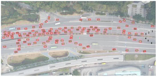
Figure 1. Processing diagram of unstructured data.

After filtering trajectories without lane numbers and trajectories with lane number changes, a total of 306 valid track-following straight trajectory data were obtained. The relationship between the continuous driving velocity of the vehicle and the distances to the (1) right and (2) front of the vehicle were obtained by fitting, as shown in Figure 2.

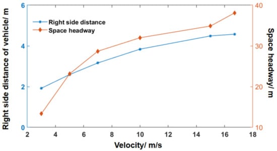
Figure 2. Relationship of vehicle velocity to forward and lateral distances.

From Figure 2, it can be observed that there is an evident correlation between the velocity and the distance of the vehicle in the forward and lateral distances. During the driving process of the vehicle, as the space headway to the leading vehicle decreases, the rear vehicle will be stimulated to slow down. Similarly, the closer the vehicle is to the sideways vehicle, the greater the incentive for the driver to slow down. Simultaneously, the desired following distance of the vehicle is intruded, prompting a larger deceleration. There are also differences in the PS of different drivers, resulting in the irregular curved shape observed in Figure 2.

Therefore, the forward and lateral distances of the vehicle are important factors affecting the vehicle’s following behavior. To study the influence mechanism of this factor on traffic flow stability, the car-following model is established.

3. Car-Following IDM Considering PS

PS is variable and regional. Currently, the quantitative calculation method for the shape and distance of PS has not been determined. Hecht et al. [17] proved through the simple stopping distance method that the boundary of PS is approximately circular. Furthermore, the results of anisotropic testing showed that the human anterior thoracic area has a larger demand for space than the back area [18]. This paper focuses on the forward and lateral distances of the vehicle. An egg-shaped boundary is defined based on the above elliptical boundary. The variability is determined by the velocity of the vehicle and individual driver differences. The regionality is determined by the PS boundary formula expressed in Equation (1) below.

$$S_i\left(t\right)=\left\{\begin{array}{c}\frac{{\left(x-x_i\left(t\right)\right)}^2}{A_i{\left(t\right)}^2}+\frac{{\left(y-y_i\left(t\right)\right)}^2}{B_i{\left(t\right)}^2}\le 1,x\ge x_i\left(t\right)\\ \frac{{\left(x-x_i\left(t\right)\right)}^2+{\left(y-y_i\left(t\right)\right)}^2}{B_i{\left(t\right)}^2}\le 1,x<x_i\left(t\right)\end{array}\right.$$

(1)

where $S_i(t)$ is the PS boundary of vehicle $i$ at time $t$; $x_i(t)$ and $y_i(t)$ are the coordinates of vehicle $i$ at time $t$; $x$ and $y$ are points on the PS boundary; $A_i$ is the forward distance of vehicle $i$; and $B_i$ is the lateral distance of vehicle $i$. The specific shapes are shown in Figure 3.

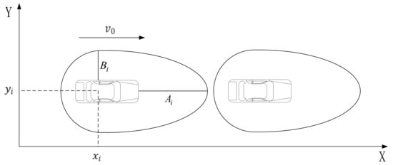
Figure 3. PS boundary of vehicle.

Based on the intelligent driver model (IDM) [8], as shown in Equation (2), and by considering the influence of PS on car-following behavior, a PS-IDM analytical model of car-following behavior is established, as shown in Equation (3).

$$\left\{\begin{array}{c}\dot{v}=a\left[1-{\left(\frac{v_0}{v_f}\right)}^4-{\left(\frac{s_1}{h-l}\right)}^2\right]\\ s_1=s_0+v_0{T}_s+\frac{v_0\Delta v}{2\sqrt{ab}}\end{array}\right.$$

(2)

where $\dot{v}$ is the vehicle acceleration; $v_0$ is the current velocity of the vehicle; $a$ is the maximum acceleration; $v_f$ is the free-flow velocity; $s_1$ is the desired vehicle distance; $h$ is the current space headway of the vehicle; $l$ is the vehicle length; $s_0$ is the minimum parking distance; $T_s$ is the safe time headway; $\Delta v$ is the velocity difference from the vehicle ahead; and $b$ is the comfortable deceleration.

Based on literature review and test analysis, PS has excellent coupling with car-following model. Considering the effects of $A_i$ and $B_i$ in Equation (2), the following equation for the car-following behavior was obtained.

$$\left\{\begin{array}{c}\dot{v}=a\left[1-{\left(\frac{v_0}{v_f}\right)}^4-{\left(\frac{s_1}{h-l}\right)}^2\right]+\lambda c_i\\ s_1=s_0+v_{0}T+\frac{v_0\Delta v}{2\sqrt{ab}}\end{array}\right.$$

(3)

In Equation (3), the time headway is an intuitive representation of the longitudinal dimension of the driver’s difference, i.e., $A_i$ denotes the corrected time headway $T=T_s+\Delta T$, and $\Delta T$ is the time headway correction value. $B_i$ denotes the lateral distance factor term $\lambda c_i$, $\lambda$ is the lateral distance utility parameter, and $c_i$ is the lateral intrusion distance of vehicle $i$. As shown in Figure 4, the intrusion distance is related to the vehicle position and the current velocity.

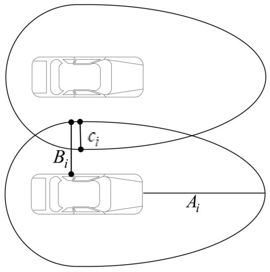
Figure 4. Schematic diagram of intrusion rate.

4. Conditions for Stability Judgment

The equilibrium velocity of the traffic flow is defined as $v_e$, and the space headway of the traffic flow is defined as equilibrium $h_e$. By considering only the velocity disturbance $v_n(t)-v_e$ and the inter-vehicle distance disturbance $h_n(t)-h_e$ in the traffic flow, the first-order Taylor expansion of the model at $f(h_e,v_e,0)$ was obtained. Subsequently, the IDM traffic flow disturbance transfer function was derived from the Laplace transform of the velocity input signal and the Laplace transform of the velocity output signal.

The disturbance transfer function in the equilibrium state of traffic flow is expressed in Equation (4) as follows.

$$F\left(S\right)=\frac{f_{\Delta v}S+f_h}{S^2+\left(f_{\Delta v}-f_{v_0}\right)S+f_h}$$

(4)

where $S$ is the Laplace domain, and $f_{\Delta v}$, $f_h$, and $f_{v_0}$ are the partial differentials of $\Delta v$, $h$ and $v_0$, respectively, in Equation (3).

Subsequently,$f_{\Delta v}$, $f_h$, and $f_{v_0}$ are substituted to obtain the disturbance transfer function $F\left(S_1\right)$ of the car-following model of the HD.

$$F\left(S_1\right)=\frac{\sqrt{\frac{a}{b}}\frac{v_{\mathrm{e}}\left[1-{\left(v_{\mathrm{e}}/v_f\right)}^4\right]}{s_0+v_{\mathrm{e}}T}S+2a\frac{\left[1-{\left(v_{\mathrm{e}}/v_f\right)}^4\right]\sqrt{\left[1-{\left(v_{\mathrm{e}}/v_f\right)}^4\right]}}{s_0+v_{\mathrm{e}}T}}{S^2+\left(\sqrt{\frac{a}{b}}\frac{v_{\mathrm{e}}\left[1-{\left(v_{\mathrm{e}}/v_f\right)}^4\right]}{s_0+v_{\mathrm{e}}T}+\frac{4a{v_{\mathrm{e}}}^3}{v_f^4}+\frac{2aT\left[1-{\left(v_{\mathrm{e}}/v_f\right)}^4\right]}{s_0+v_{\mathrm{e}}T}-\lambda \frac{\mathrm{d}{c}_i}{\mathrm{d}{v}_{\mathrm{e}}}\right)S+2a\frac{\left[1-{\left(v_{\mathrm{e}}/v_f\right)}^4\right]\sqrt{\left[1-{\left(v_{\mathrm{e}}/v_f\right)}^4\right]}}{s_0+v_{\mathrm{e}}T}}$$

(5)

The feedback information of the preceding vehicle is added based on the CACC car-following model, and the acceleration of the preceding vehicle is often ignored in the car-following model. In this study, the acceleration feedback coefficient $r\left(0\le r\le 1\right)$ of the preceding vehicle was added to derive the disturbance transfer of the CACC car-following model. The function is given by Equation (6).

$$F\left(S_2\right)=\frac{r{S}^2+\sqrt{\frac{a}{b}}\frac{v_{\mathrm{e}}\left[1-{\left(v_{\mathrm{e}}/v_f\right)}^4\right]}{s_0+v_{e}T}S+2a\frac{\left[1-{\left(v_{\mathrm{e}}/v_f\right)}^4\right]\sqrt{\left[1-{\left(v_{\mathrm{e}}/v_f\right)}^4\right]}}{s_0+v_{\mathrm{e}}T}}{S^2+\left(\sqrt{\frac{a}{b}}\frac{v_{\mathrm{e}}\left[1-{\left(v_{\mathrm{e}}/v_f\right)}^4\right]}{s_0+v_{\mathrm{e}}T}+\frac{4a{v_{\mathrm{e}}}^3}{v_f^4}+\frac{2aT\left[1-{\left(v_{\mathrm{e}}/v_f\right)}^4\right]}{s_0+v_{\mathrm{e}}T}-\lambda \frac{\mathrm{d}{c}_i}{\mathrm{d}{v}_{\mathrm{e}}}\right)S+2a\frac{\left[1-{\left(v_{\mathrm{e}}/v_f\right)}^4\right]\sqrt{\left[1-{\left(v_{\mathrm{e}}/v_f\right)}^4\right]}}{s_0+v_{\mathrm{e}}T}}$$

(6)

where $r$ is acceleration feedback coefficient of CACC vehicles.

In the mixed traffic flow, $F\left(S_1\right)$ and $F\left(S_2\right)$ act together; let $S=jw$ according to the following system stability conditions [7]:

$$\begin{array}{cc}\hfill & {\left|F\left(S\right)\right|}_{\infty }={\left|F\left(jw\right)\right|}_{\infty }={\left|F_1{\left(jw\right)}^{(1-p)}{F}_2{\left(jw\right)}^p\right|}_{\infty }\hfill \\ \hfill & ={\left(\frac{f_{\Delta v}jw+f_h}{-w^2+\left(f_{\Delta v}-f_{v_0}\right)jw+f_h}\right)}^{(1-p)}{\left(\frac{-r{w}^2+f_{\Delta v}jw+f_h}{-w^2+\left(f_{\Delta v}-f_{v_0}\right)jw+f_h}\right)}^p\hfill \\ \hfill & ={\left(\frac{\sqrt{{\left(f_{\Delta v}w\right)}^2+{\left(f_h\right)}^2}}{\sqrt{{\left(f_{\Delta v}-f_{v_0}\right)}^2{w}^2+{\left(f_h-w^2\right)}^2}}\right)}^{(1-p)}{\left(\frac{\sqrt{{\left(f_{\Delta v}w\right)}^2+{\left(f_h-r{w}^2\right)}^2}}{\sqrt{{\left(f_{\Delta v}-f_{v_0}\right)}^2{w}^2+{\left(f_h-w^2\right)}^2}}\right)}^p\le 1\hfill \end{array}$$

(7)

where $j$ and $w$ are imaginary numbers and frequencies of frequency domains, ${\left|·\right|}_{\infty }$ is the maximum amplitude of transfer function frequency domain, $p$ is the penetration rate of the CACC vehicle.

The notations involved in the model are shown in Table 2.

Table 2. Notations Summary Table.

Notation	Definition
$S_i(t)$	PS boundary of vehicle $i$ at time $t$
$x_i(t)$	Horizontal coordinates of vehicle $i$ at time $t$
$y_i(t)$	Horizontal coordinates of vehicle $i$ at time $t$
$x$	Points on the PS boundary
$y$	Points on the PS boundary
$A_i$	The forward distance of vehicle $i$
$B_i$	The lateral distance of vehicle $i$
$\dot{v}$	Vehicle acceleration
$v_0$	The current velocity of the vehicle
$a$	Maximum acceleration
$v_f$	Free-flow velocity
$s_1$	Desired vehicle distance
$h$	The current space headway of the vehicle
$l$	Vehicle length
$s_0$	Minimum parking distance
$T_s$	Safe time headway
$\Delta v$	Velocity difference
$b$	Comfortable deceleration
$\Delta T$	Time headway correction value
$T$	Corrected time headway
$c_i$	Lateral intrusion distance
$\lambda$	Lateral distance utility parameter
$F\left(S\right)$	Disturbance transfer function
$S$	Laplace domain
$f_{\Delta v}$	Partial differentials of $\Delta v$
$f_h$	Partial differentials of $h$
$f_{v_0}$	Partial differentials of $v_0$
$v_e$	Equilibrium velocity
$h_e$	Equilibrium space headway
$F\left(S_1\right)$	Disturbance transfer function of HD
$F\left(S_2\right)$	Disturbance transfer function of CACC
$r$	Acceleration feedback coefficient
$j$	Imaginary number
$w$	Frequency of frequency domain
$p$	Penetration rate of CACC vehicle

5. Stability Analysis of Mixed Traffic Flow Based on PS-IDM

We performed a theoretical analysis on the stability of the car-following model and introduced PS-IDM with different values to analyze the stability of homogeneous and heterogeneous traffic flow and explored the influence of PS on the stability of traffic flow.

5.1. Model Parameter Calibration

In the model, the following parameter values were assigned according to Milanés and Shladover [11]: $a$ = 1 m/s², $v_f$ = 33.3 m/s, $l$ = 5 m, and $S_0$ = 2 m. The value of $b$ for the HD and CACC vehicles were 2 and 2.8 m/s, respectively. [19]. The time headway correction value $\Delta T$ and lateral distance utility parameters $\lambda$ were calibrated using actual survey data.

When the time headway was greater than 3 s, the front and rear cars were less restrictive. After screening, 292 groups of valid data from the test analysis were extracted, with the time headway being between 0 and 3 s. To obtain the time headway correction value of different driver personalities, the data were clustered and analyzed based on the k-means algorithm. The driving styles of drivers are usually classified into three categories: aggressive, ordinary, and conservative [20]. Therefore, a clustering number of 3 was used. The results for clusters 1, 2, and 3 were 2.2, 1.6, and 1.1, respectively, and are shown in Figure 5.

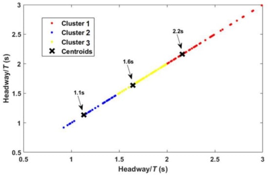
Figure 5. k-means cluster analysis diagram.

Based on the above analysis, the longitudinal stability study was conducted to explore individual differentiation at the values of 2.2, 1.6, and 1.1 s.

The difference between the maximum abscissas under free flow conditions was screened, and it was assumed that the current driver had obtained enough personal space, and the difference between the vehicle velocity and the abscissa was fitted to obtain the mathematical relationship between $v_0$ and $2B_i$. The lateral direction of PS was obtained through further processing. The relationship between distance $B_i$ and vehicle velocity $v_0$ is shown in Equation (8).

$$B_i=0.029v_0+0.7364$$

(8)

where $B_i$ is the lateral distance of the vehicle $i$, $i$ is the vehicle number, and $v_0$ is the current velocity of the vehicle.

$B_i$ was substituted into the second item $\frac{{\left(x-x_i\left(t\right)\right)}^2+{\left(y-y_i\left(t\right)\right)}^2}{B_i{\left(t\right)}^2}\le 1$ of Equation (1) to obtain the partial PS boundary of vehicle $i$ at $x<x_i\left(t\right)$, which was used to quantify $c_i$, the lateral intrusion distance of vehicle i, as expressed in Equation (9).

$$c_i=\frac{\left(B_i+B_{i+1}+k\right)-\left|y_i-y_{i+1}\right|}{2}$$

(9)

where $B_{i+1}$ is the PS lateral distance of the laterally adjacent vehicle, $k$ is the width of the vehicle, $y_i$ is the ordinate of the vehicle, $y_{i+1}$ is the ordinate of the laterally adjacent vehicle, and $i+1$ is the number of the laterally adjacent vehicle.

$c_i$ was substituted into Equation (3), and, using the nonlinear regression (nlinfit) and nonlinear curve fitting (lsqcurvefit) functions of Matlab to fit the two values of deceleration $b$, the HD vehicle lateral distance utility parameter was found to be 0.055. Similarly, the CACC vehicle lateral distance utility parameter was 0.048. The fitting residual error, the sums of squares, were all less than 0.001.

The results of parameter calibration are shown in Table 3.

Table 3. Parameter value.

Parameter Name	Parameter Notation	Parameter Value (Unit)
Maximum acceleration	$a$	1 (m/s2)
Comfortable deceleration	$b$	2 or 2.8 (m/s2)
Free-flow velocity	$v_f$	33.3 (m/s)
Vehicle length	$l$	5 (m)
Vehicle width	$k$	2 (m)
Minimum parking distance	$s_0$	2 (m)
Corrected time headway	$T$	1.6, 1.8, 2.2(s)
Lateral distance utility function	$\lambda$	0.055 or 0.048

5.2. Stability Analysis

5.2.1. Homogeneous Traffic Flow

In Equation (7), when $p=0$, it degenerates to a homogeneous HDV traffic flow; when $p=1$, it degenerates to a homogeneous CACC vehicle traffic flow stability condition.

Based on Equation (7) and $\forall w>0$, the stability conditions of the homogeneous HDV traffic flow are given by Equation (10) below.

$$\begin{array}{l}{f}_1=\frac{1}{2}{\left(-\frac{4a{v}_e{}^3}{v_f^4}-\frac{2aT\left[1-{\left(v_e/v_f\right)}^4\right]}{s_0+v_{e}T}+{\lambda }_1\frac{\mathrm{d}{c}_i}{\mathrm{d}{v}_{\mathrm{e}}}\right)}^2-\left(\sqrt{\frac{a}{b}}\frac{v_e\left[1-{\left(v_e/v_f\right)}^4\right]}{s_0+v_{e}T}\right)\left(-\frac{4a{v}_e{}^3}{v_f^4}-\frac{2aT\left[1-{\left(v_e/v_f\right)}^4\right]}{s_0+v_{e}T}+{\lambda }_1\frac{\mathrm{d}{c}_i}{\mathrm{d}{v}_{\mathrm{e}}}\right)-\\ 2a\frac{\left[1-{\left(v_e/v_f\right)}^4\right]\sqrt{\left[1-{\left(v_e/v_f\right)}^4\right]}}{s_0+v_{e}T}\ge 0\end{array}$$

(10)

When the free flow velocity is 0–33.3 m/s, the stability of HDV at different equilibrium velocities at $T$ = 1.1 s, $T$ = 1.6 s, and $T$ = 2.2 s is analyzed by using Equation (10), as shown in Figure 6.

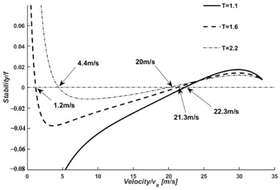
Figure 6. Analytical diagram of the stability of homogeneous HD traffic flow.

It can be observed from Figure 6 that homogeneous HDV traffic flow is unstable at 0~22.3 m/s when the value of is 1.1 s; the homogeneous HDV traffic flow is unstable at 1.2~21.3 m/s when the value of $T$ is 1.6 s; the homogeneous HDV traffic flow is unstable at 4.4~20 m/s when $T$ is 2.2 s. With an increase in $T$ value, the unstable velocity range of the homogeneous HDV traffic flow is gradually reduced. Furthermore, traffic flow tends to be stable, regardless of the value of $T$. However, when $T$ is 2.2 s, the traffic flow transforms into a stable state the fastest.

Similarly, the stability condition of the traffic flow of homogeneous CACC vehicles should satisfy Equation (11).

$$\begin{array}{l}{f}_2=\frac{1}{2}{\left(-\frac{4a{v}_e{}^3}{v_f^4}-\frac{2aT\left[1-{\left(v_e/v_f\right)}^4\right]}{s_0+v_{e}T}+{\lambda }_2\frac{\mathrm{d}{c}_i}{\mathrm{d}{v}_{\mathrm{e}}}\right)}^2-\left(\sqrt{\frac{a}{b}}\frac{v_e\left[1-{\left(v_e/v_f\right)}^4\right]}{s_0+v_{e}T}\right)\left(-\frac{4a{v}_e{}^3}{v_f^4}-\frac{2aT\left[1-{\left(v_e/v_f\right)}^4\right]}{s_0+v_{e}T}+{\lambda }_2\frac{\mathrm{d}{c}_i}{\mathrm{d}{v}_{\mathrm{e}}}\right)-\\ \left(1-r\right)2a\frac{\left[1-{\left(v_e/v_f\right)}^4\right]\sqrt{\left[1-{\left(v_e/v_f\right)}^4\right]}}{s_0+v_{e}T}\ge 0\end{array}$$

(11)

The sensitivity analysis of CACC vehicle acceleration feedback coefficients $r$ = 0.1, $r$ = 0.2, and $r$ = 0.3 is shown in Figure 7. Figure 7a–c show the stability at $T$ = 1.1 s, $T$ = 1.6 s, and $T$ = 2.2 s, respectively.

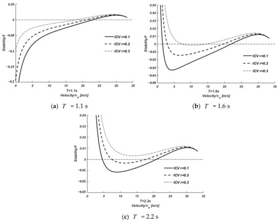
Figure 7. Analytical diagram of the stability of homogeneous CACC vehicles traffic flow.

Figure 7a shows that the unstable velocity range gradually decreases in the case of $T$ = 1.1 s with an increase in $r$. When $r$ = 0.1, the stability of the homogeneous CACC vehicle traffic flow increases with the velocity, reaching the zero point at 23 m/s. The unstable state turns to a stable state, and then it is stable within the free flow velocity. When $r$ = 0.2, the stable zero point of the homogeneous CACC vehicle traffic flow shifts to the left, which is unstable at 0~21 m/s, and stabilizes after the traffic velocity exceeds 21 m/s. When $r$ = 0.3, the unstable velocity boundary continues to shrink, and the zero-boundary point moves to the right to 17.9 m/s.

Figure 7b shows that the traffic flow of homogeneous CACC vehicles is stable in the initial stage and then gradually decreases, when $r$ = 0.1, in the case of $T$ = 1.6 s. It reaches the first zero boundary point at 1.6 m/s and becomes unstable. This state continues to reach the second zero boundary point at 22 m/s, and then it is stable until 33.3 m/s; when $r$ = 0.2, the first zero boundary point moves to the right, and the second zero boundary point moves to the left. The unstable velocity range of the CACC vehicle is 3~19.6 m/s; when $r$ = 0.3, the traffic flow is only unstable at 7.5~14.5 m/s.

Figure 7c shows that the stability of the homogeneous CACC vehicles’ traffic flow gradually decreases within 0~4.6 m/s, and the traffic flow starts to be unstable at 4.6 m/s and stabilizes when the velocity reaches 20.8 m/s, when $r$ = 0.1, in the case of $T$ = 2.2 s; when $r$ = 0.2, the unstable velocity range is reduced, the left boundary is shifted to 7.5 m/s, and the right boundary is shifted to 17.5 m/s; when $r$ = 0.3, homogeneous CACC vehicles traffic flow is stable within the free flow velocity range.

5.2.2. Heterogeneous Traffic Flow

According to the discrimination conditions in Section 4, the discrimination conditions for the stability of heterogeneous traffic flow can be generalized using Equations (10) and (11) to obtain Equation (12) as follows.

$$f=\left(1-p\right)f_1+p{f}_2\ge 0$$

(12)

where $f$ is the stability of heterogeneous traffic flow, $f_1$ and $f_2$ are each the stability of homogeneous traffic flow, and $p$ is the penetration rate of the CACC vehicle.

Using a homogeneous traffic flow analysis method to adjust the CACC vehicle penetration rate, the mixed traffic flow stability region under different CACC vehicle penetration rates and different equilibrium velocities can be calculated. As shown in Figure 8, the stable region conditions for four types of $r$ values and three types of $T$ values are given. The black area in the figure is the unstable area, and the white area outside the black area is the stable area. In Figure 8, when the CACC vehicle penetration rate is 0, the boundary value of the black unstable area and the white stable area is the velocity boundary value of the homogeneous HDV traffic flow. It can be obtained from the analysis results in Figure 6.

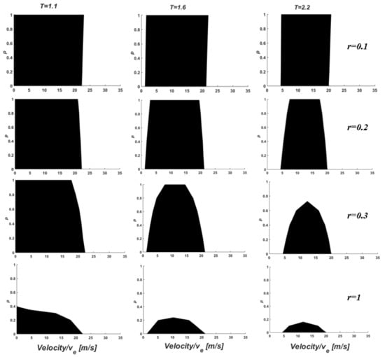
Figure 8. Stability region of heterogeneous traffic flow.

As shown in Figure 8, when the CACC vehicle penetration rate is 1, the velocity boundary and the values of $r$ are negatively correlated, i.e., the larger the value of $r$, the smaller the unstable velocity range of the CACC vehicle. When $r$ = 0.1, the velocity boundaries are 0~23 m/s, 1.6~22 m/s, and 4.6~20.8 m/s, corresponding to $T$ = 1.1 s, 1.6 s, and 2.2 s, respectively. When $r$ = 0.2, the velocity boundaries are 0~21 m/s, 3~19.6 m/s, and 7.5~17.5 m/s, corresponding to $T$ = 1.1 s, 1.6 s, and 2.2 s, respectively. When $r$ = 0.3, $T$ = 1.1 s and 1.6 s correspond to the velocity boundaries 0~17.9 m/s and 7.5~14.5 m/s, respectively. When the value of $T$ is 2.2 s, the traffic flow of homogeneous CACC vehicles is stable in the free-flow velocity range. When $r$ = 1, the unstable region is the smallest.

Therefore, under the same value of $T$, as the feedback coefficient $r$ increases, the unstable region of heterogeneous traffic flows shrinks. Furthermore, under the same value of $r$, with an increase in time headway $T$, the unstable region of heterogeneous traffic flow is significantly reduced.

For each individual unstable domain, when $r$ ≥ 0.2, the traffic flow instability region of homogeneous CACC vehicles is within the homogeneous HDV traffic flow instability region, i.e., in the homogeneous HDV traffic flow stability region, and the heterogeneous traffic flow of any CACC vehicle permeability is stable. Especially, when $r$ = 0.1, the unstable velocity range of the homogeneous CACC vehicle traffic flow is slightly larger than that of the homogeneous HD traffic flow.

Until $r$ = 0.3, $T$ = 2.2, $p$ ≥ 0.72, a constant stability region appears. When $r$ = 1, the CACC vehicle penetration rate reaches 0.395, 0.24, and 0.16, and the heterogeneous traffic flow is stable within the free flow velocity range of $T$ = 1.1 s, 1.6 s, and 2.2 s, respectively.

6. Model Validation Analysis

We used a Matlab simulation experiment, compared with the IDM model, to analyze the effect of the PS-IDM model proposed in this paper on the stability of mixed traffic flow, to verify the correctness of the theoretical analysis.

Based on the international standard ISO2631-1 [21] related to human body vibration evaluation and driving comfort standards, the driving comfort during the disturbance propagation process of the car-following model in this study was evaluated, and the traffic flow stability was quantitatively evaluated. The driving comfort index can be calculated using Equation (13) as follows.

$$CI=\sqrt{\frac{1}{m}{\displaystyle {\sum }_{i=0}^m{a}_i^2}}$$

(13)

where $CI$ is the driving comfort index, $a_i$ is the acceleration value of each vehicle obtained by statistics, and $m$ is the total acceleration statistic. This index uses the root mean square value of the total vibration acceleration to determine the comfort of the occupants. The smaller the value of $CI$, the better the driving comfort, and vice versa, which verifies the consistency of the analytical results with the stability theory.

Secondly, the intrusion rate index was used to evaluate the impact of lateral intrusion of adjacent vehicles into the PS, and to explore the internal relationship between the intrusion rate and longitudinal stability. Further, this index was used to study the lateral stability of the PS. The formula for calculating the intrusion rate is expressed in Equation (14).

$$I=\frac{c}{l_a}\times 100\%$$

(14)

where $I$ is the percentage index of the invasion rate, $c$ is the invasion length, and $l_a$ is the length of the PS in the invasion direction.

$l_a$ is equal to the lateral distance of the vehicle PS $B_i$. Therefore, Equation (14) can be rewritten as:

$$I=\frac{c_i}{B_i}\times 100\%$$

(15)

The smaller the value of $I$, the smaller the PS intrusion rate, and the lower the effect on the vehicle PS. Conversely, the higher the intrusion rate, the greater the impact.

6.1. Experimental Design

A MATLAB simulation experiment was used to analyze the stability state of the mixed traffic flow of the disturbance transfer function under different CACC vehicle permeabilities. According to the analysis results of the stability of heterogeneous traffic flow in Section 5.2.2, the acceleration feedback coefficient of preceding vehicle $r$ is set to 0.3, and the experimental results are satisfactory and without loss of generality. Based on MATLAB numerical simulation, the effectiveness of the PS-IDM proposed in this study is compared with that of a single IDM.

In the simulation experiment, the number of HD and CACC vehicles was determined using the set $p$ value, and 50 vehicles were randomly placed on a 200 m single-lane road. Initially, the hybrid platoon drove at the equilibrium velocity $v_e$, and then a disturbance was generated by randomly slowing down to break the equilibrium state. The disturbance propagates in pairs in the platoon, based on the disturbance transfer function. In the propagation process, the operating status of each vehicle was obtained, and the acceleration and distance between the heads of the vehicle were extracted to calculate the relevant indicators. According to the above stability analysis results, HD vehicles are always unstable at 4.4~20 m/s. To analyze the influence of CACC vehicles on the instability of HDV traffic flow, the initial equilibrium velocity of the fleet was selected as 10 m/s for the numerical simulation. The random slowdown probability was set to 0.3, the simulation step length was set to 0.1 s, and comfort was selected as the evaluation index of the simulation experiment.

6.2. Simulation Results

The results of the numerical simulation experiments are listed in Table 4. Taking the $r$ value of 0.3, the comfort index was calculated, and the results are shown in the tables below.

Table 4. PS-IDM and Single IDM comfort index.

$\mathit{p}$	$\mathit{C}\mathit{I}$
	$\mathit{T}$ = 1.1 s	$\mathit{T}$ = 1.6 s	$\mathit{T}$ = 2.2 s
		PS-IDM
0	0.33466	0.27424	0.17642
0.2	0.17434	0.14027	0.08766
0.4	0.16462	0.13556	0.07046
0.6	0.14485	0.13085	0.06436
0.8	0.12084	0.11800	0.05064
1	0.11846	0.09342	0.04978
		Single IDM
0	0.34465	0.28498	0.18776
0.2	0.17647	0.14648	0.09349
0.4	0.16894	0.14064	0.07309
0.6	0.14698	0.13584	0.06618
0.8	0.13649	0.12986	0.06036
1	0.34465	0.28498	0.18776

It can be noted from Table 4 and Figure 9 that the higher the penetration rate of CACC vehicles, the higher the driving comfort under the same $T$ value.

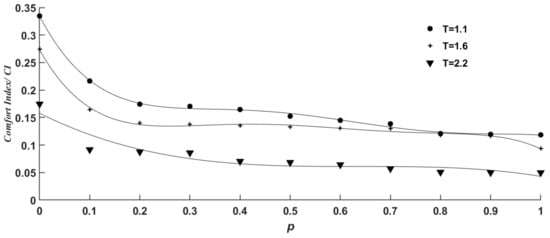
Figure 9. Scatter plot of PS-IDM comfort index.

Compared with the homogeneous CACC vehicle traffic flow, the $CI$ value of the homogeneous HD traffic flow was reduced by 64.67, 66.06, and 72.16% when $T$ = 1.1, 1.6, and 2.2 s, respectively. The results showed that an increase in PS improved driving comfort, which was consistent with the analytical results of the longitudinal stability theory.

Figure 10 shows a comparison chart of the comfort index during the simulation process of the PS-IDM and single IDM models. The solid line is the PS-IDM comfort index fitting curve, and the dashed line is the single IDM comfort index fitting curve. Under the same circumstances, the $CI$ value of a single IDM is greater than the $CI$ value of the PS-IDM. Compared with a single IDM, the comfort of the PS-IDM can be increased by up to 20.7%.

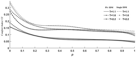
Figure 10. Comparison chart of the index before and after model improvement.

The intrusion rate of each vehicle was discrete data, and the simulation experiment was performed using MATLAB. In addition, the average value of the intrusion rate of 50 for the simulated vehicles was taken as the simulation result of the intrusion rate index. Taking $T$ = 1.1 s and $r$ = 0.3 as an example, the result is shown in Figure 11.

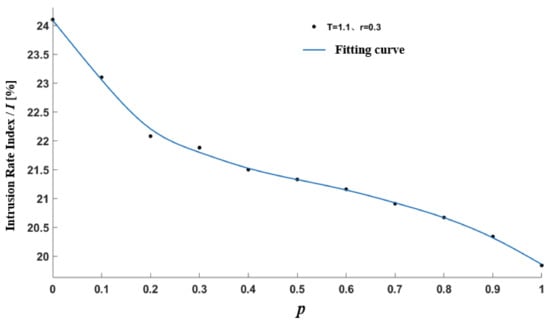
Figure 11. Fitting curve of average intrusion rate.

In Figure 11, when the HD vehicle traffic flow is homogeneous, the average intrusion rate is higher than 24%. As the penetration rate of CACC vehicles increases, the intrusion rate decreases, when the traffic flow of the homogenous HD vehicle changes to the traffic flow of homogenous CACC vehicles. In particular, at the beginning of the transition period ($p\in \left(0,0.3\right)$), the downward trend is evident. When the mixed traffic flow degenerates into a homogenous CACC vehicle traffic flow ($p=1$), the average intrusion rate drops to 19.4%.

The simulation results show that there is a positive correlation between the intrusion rate index and the comfort index. The smaller the value of the comfort index, the smaller the intrusion rate index value, and the better the driving stability, which is consistent with the analytical results of the lateral stability theory.

7. Conclusions

(1) Aiming at the HD-CACC mixed traffic flow, this study establishes a car-following PS-IDM model based on an intelligent driver model by considering personal space. Using theoretical analysis and MATLAB simulation experiments, the stability regions of homogeneous traffic flows under different PS and heterogeneous traffic flows with different CACC vehicle permeabilities were analyzed. The results show that the PS-IDM model can improve the driving comfort by up to 20.7% compared with a single IDM model, and the average PS intrusion rate is reduced by 4.6%, which verifies the effectiveness of the PS-IDM model.

(2) The analytical results of the traffic flow stability of car-following behavior, considering PS, indicates that the unstable velocity range of homogeneous or heterogeneous traffic flows decreases with an increase in PS. In addition, the unstable velocity range of the CACC vehicle traffic flow has a negative correlation with the acceleration feedback coefficient. The increased penetration rate of CACC vehicles with the acceleration feedback coefficient below 0.2 could not turn an unstable traffic flow into a stable traffic flow; when the acceleration feedback coefficient exceeded 0.2, the increase in CACC vehicle permeability can effectively transform the stability of traffic flow. Regardless of the value of the acceleration feedback coefficient, increasing the time headway can make the traffic flow to a stable state. Therefore, an increase in the longitudinal distance of the vehicle PS is beneficial to the stability of the traffic flow.

(3) The results of the numerical simulation experiments were consistent with the analytical results of the stability theory. The model and experiment in this study made assumptions regarding the lane conditions. In the future, we will analyze the lateral factors influencing the multi-lane situation and conduct in-depth research on the lateral distance. In addition, because different values of the acceleration feedback coefficient can correspond to HD, multi-level individual intelligent vehicles, and multi-level connected automated vehicles, further analysis and research on the stability of complex heterogeneous traffic flows will be conducted.

References

- Petrillo, A.; Pescapé, A.; Santini, S. A collaborative approach for improving the security of vehicular scenarios: The case of platooning. Comput. Commun. 2018, 122, 59–75. [Google Scholar] [CrossRef]
- Hu, X.; Zheng, M. Research progress and prospects of vehicle driving behavior prediction. World Electr. Veh. J. 2021, 12, 88. [Google Scholar] [CrossRef]
- Reuschel, A. The Movement of a Column of Vehicles when the Leading Vehicle Is Uniformly Accelerated or Decelerated. Mag. Austrian Eng. Archit. Assoc. 1950, 4, 193–215. [Google Scholar]
- Hoogendoorn, S.P.; Bovy, P.H.L. State-of-the-art of vehicular traffic flow modelling. Proc. Inst. Mech. Eng. Part I J. Syst. Control. Eng. 2001, 215, 283–303. [Google Scholar] [CrossRef]
- Yang, L.H.; Zhang, C.; Qiu, X.B.; Li, S.; Wang, H. Research progress on car-following models. J. Traffic Transp. Eng. 2019, 19, 125–138. [Google Scholar]
- Bando, M. Dynamical model of traffic congestion and numerical simulation. Phys. Rev. E 1995, 51, 1035–1042. [Google Scholar] [CrossRef] [PubMed]
- Jiang, R.; Wu, Q.S.; Zhu, Z.J. Full velocity difference model for a car-following theory. Phys. Rev. E 2001, 64, 017101. [Google Scholar] [CrossRef] [PubMed]
- Treiber, M.; Hennecke, A.; Helbing, D. Congested traffic states in empirical observations and microscopic simulations. Phys. Rev. E 2000, 62, 1805–1824. [Google Scholar] [CrossRef]
- Qin, Y.Y.; Hu, X.H.; Li, S.Q.; He, Z.Y.; Xu, M.T. Stability analysis of mixed traffic flow in connected and autonomous environment. J. Harbin Inst. Technol. 2021, 3, 152–157. [Google Scholar]
- Saifuzzaman, M.; Zheng, Z.; Haque, M.M.; Washington, S. Revisiting the Task–Capability Interface model for incorporating human factors into car-following models. Transp. Res. Part B Methodol. 2015, 82, 1–19. [Google Scholar] [CrossRef]
- Milanés, V.; Shladover, S.E. Modeling cooperative and autonomous adaptive cruise control dynamic responses using experimental data. Transp. Res. Part C Emerg. Technol. 2014, 48, 285–300. [Google Scholar] [CrossRef]
- Editorial office of China Journal of Highway and Transport. Review on China’s Traffic Engineering Research Progress: 2016. China J. Highw. Transp. 2016, 29, 1–161. [Google Scholar]
- Edward, T.H. The Hidden Dimension; Anchor Books Publishing: New York, NY, USA, 1982. [Google Scholar]
- Pham, Q.T. Investigation of Avoidance Assistance System for the Driver of a Personal Transporter Using Personal Space: A Simulation Based Study. Int. J. Mech. Eng. Robot. Res. 2019, 8, 254–259. [Google Scholar]
- Sun, J.; Zheng, Z.; Sun, J. Stability analysis methods and their applicability to car-following models in conventional and connected environments. Transp. Res. Part B Methodol. 2018, 109, 212–237. [Google Scholar] [CrossRef]
- Dai, J.; Li, Y.; He, K.; Sun, J. Object Detection via Region-Based Fully Convolutional Networks. arXiv 2016, arXiv:1605.06409. [Google Scholar]
- Hecht, H.; Welsch, R.; Viehoff, J.; Longo, M. The shape of personal space. Acta Psychol. 2019, 193, 113–122. [Google Scholar] [CrossRef] [PubMed]
- Welsch, R.; Castell, C.; Hecht, H. The anisotropy of personal space. PLoS ONE 2019, 14, e0217587. [Google Scholar] [CrossRef] [PubMed]
- Shladover, S.; Su, D.; Lu, X.Y. Impacts of Cooperative Adaptive Cruise Control on Freeway Traffic Flow. Transp. Res. Rec. 2012, 2324, 63–70. [Google Scholar] [CrossRef]
- Milad, M.; Saleh, A.; Trond, N. A hybrid speed choice model: The role of human factors. Transp. Lett. 2023, 15, 152–161. [Google Scholar]
- ISO2631-1; Mechanical Vibration and Shock—Evaluation of Human Exposure to Whole-Body Vibration—Part 1: General Requirements. ISO: Geneva, Switzerland, 2010.
Disclaimer/Publisher’s Note: The statements, opinions and data contained in all publications are solely those of the individual author(s) and contributor(s) and not of MDPI and/or the editor(s). MDPI and/or the editor(s) disclaim responsibility for any injury to people or property resulting from any ideas, methods, instructions or products referred to in the content. |
© 2023 by the authors. Licensee MDPI, Basel, Switzerland. This article is an open access article distributed under the terms and conditions of the Creative Commons Attribution (CC BY) license (https://creativecommons.org/licenses/by/4.0/).