Modelling Interactions between Three Aquifer Thermal Energy Storage (ATES) Systems in Brussels (Belgium)

Featured Application

This work evaluates by numerical simulations the respective influences of three ATES systems located in two different aquifers in the center of Brussels. The model is built using Feflow©, and groundwater flow and heat transport are simulated based on all available data. The results are useful to understand how one of the systems being thermally unbalanced is influencing (i.e., decreasing in the mid- and long-term) the efficiency of the three ATES systems, even if one of them is located in a deeper aquifer.

Abstract

Shallow open-loop geothermal systems function by creating heat and cold reserves in an aquifer, via doublets of pumping and reinjection wells. Three adjacent buildings in the center of Brussels have adopted this type of aquifer thermal energy storage (ATES) system. Two of them exploit the same aquifer consisting of Cenozoic sands, and started operation in 2014 and 2017, respectively. A previous hydrogeological model developed by Bulté et al. (2021) has shown how the thermal imbalance of one of the systems jeopardizes the thermal state of this upper aquifer. Here, the interactions with a more recent third ATES system located in the deep aquifer of the Palaeozoic bedrock are studied and modelled. After being calibrated on groundwater flow conditions in both aquifers, a 3D hydrogeological model was used to simulate the cumulative effect of the three geothermal installations in the two exploited aquifers. The results of the simulations showed that although the hydraulic interactions between the two aquifers are very weak (as shown by the different observed potentiometric heads), heat exchanges occur between the two aquifers through the aquitard. Fortunately, these heat exchanges are not sufficient to have a significant impact on the efficiency of the individual geothermal systems. Additionally, this study shows clearly that adding a third system in the lower aquifer with a mean power of 286 kW for heating between October and March and an equivalent mean cooling power between April and September is efficient.

1. Introduction

The importance of renewable energy is driving a large growth in interest in geothermal systems and especially in shallow systems coupled to heat pumps. A system of groundwater pumping and reinjection performed by doublets of wells in shallow aquifers is known as Aquifer Thermal Energy Storage (ATES). In summer, groundwater is pumped into a (cold) well for cooling, and the heat is injected back with water into the aquifer at a higher temperature using a (warm) well. In winter, the system provides heat to the building from the pumped groundwater, and injection occurs at a lower temperature [1,2,3]. Both the efficiency and impact of ATES systems must be studied through the quantification of heat transfer in the saturated underground zone. Site-specific values for hydrogeological and heat transport properties/parameters are needed to design heat storage systems in aquifers. The seasonal heat storage considered in the shallow aquifers may be optimal or limited by the underground hydrodynamic conditions. If advection is driven by the hydraulic gradient and the hydraulic conductivity is high, heat and cold plumes are transferred rapidly far away from the site [4,5,6,7] so that heat/cold cannot be stored efficiently for the next season for the concerned buildings. Reliable predictions are most often based on process-based numerical simulations of groundwater flow and heat transport. A yearly annual thermal balance between cold and heat demands could be required in cases of limited heat advection.

The objective of this paper is to examine the cumulative effect of three adjacent open geothermal systems. A first model including a single aquifer, exploited by two of the three ATES systems, was developed previously by Bulté et al. [3], who studied the possible interference between these two systems. Here we add a deep aquifer separated from the upper aquifer by an aquitard (i.e., a low hydraulic conductivity layer) that is exploited by a newly added ATES system requiring a power of about 950 kW for both the cold and the warm seasons. The combined effect of the three installations is assessed with the wells of the new system established in the deeper aquifer in the fractured Paleozoic bedrock of the Brabant Massif. Heat exchanges are likely to take place through the intermediate aquitard formed by the weathered top of the bedrock, the overlying low permeability Cretaceous base deposits, and a Cenozoic clayey layer.

Here, we will demonstrate that even though one unbalanced ATES system partly jeopardizes the thermal state of the upper aquifer [3], an adjacent but deeper ATES system can operate without too many negative interactions limiting either efficiency or durability. The numerical simulation of the 3D groundwater flow and heat transport conditions considering the upper and deeper aquifers separated by the aquitard provide an excellent tool for analysis and decision support. This model will be particularly useful for the future management of the three ATES systems.

2. Materials and Methods

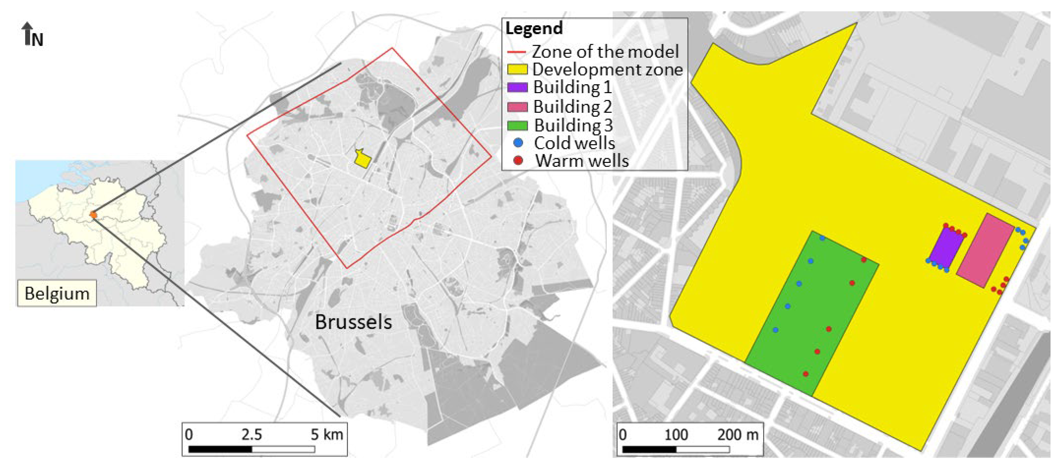
2.1. Context

When considering reductions in CO₂ emissions together with optimal cost constraints, ATES systems can be an attractive solution [8,9], especially for new or renovated buildings. The injected water temperatures induce cold and hot zones compared with the preexisting natural temperature in the aquifer. However, the long-term effects of thermal storage in the subsurface are more difficult to assess [10,11]. In very simplified and theoretical situations, the cold and hot plumes can be calculated using analytical solutions [12,13]. The complexity of actual heterogeneous hydrogeological conditions combined with the locations of the wells makes the use of coupled groundwater flow and heat transport numerical models essential [3,14,15,16,17,18,19,20,21,22,23].

Thermal interferences can be observed within one single or between neighboring systems. Depending on the site, this can have a negative or a positive impact on the performance of each system [24,25]. The negative interferences should, therefore, be avoided by adopting adequate well-to-well distances, adapting pumping/injection rates [3,4,26], and managing the energy demand toward balanced or slightly unbalanced thermal needs. Nowadays, in European countries, cooling demand may more often exceed the heating demand [27] due to climatic changes but also due to inadequate characteristics of the building or inefficient management of the heating and cooling systems. If this thermal imbalance is observed each year with pumping and injection in a low gradient and low hydraulic conductivity aquifer, the low advection will not evacuate the hot plume sufficiently from one year to another [3]. In such conditions, the cooling efficiency of the system decreases with time. In urbanized areas, a challenge consists in optimizing the systems without inducing negative interferences between them [24,25]. Other challenges concern (among others) (a) the nearly systematic oversizing of the ATES systems due mainly to future energy demand uncertainties [28], (b) the lack of monitoring data around existing ATES systems [8,29], and (c) the timing of demand for optimum building comfort conditions not corresponding to the best time for using the aquifer heat or cold storage [28,29]. Examples of geothermal reinjection technologies and modelling approaches can be found in Niknam et al. [30] and Leontidis et al. [31].

2.2. Study Case

2.2.1. Problem Statement

Three ATES systems located in two different aquifers in the center of Brussels are operated for heating and cooling three different recent or recently renovated buildings located in an urban reallocation zone of Brussels, named ‘development zone’ in Figure 1. The first one was started in March 2014 (Building 1), the second in August 2017 (Building 2), and the third (located in the deeper aquifer) in April 2020 (Building 3). The objective is to assess the potential thermal interferences between the three systems, using a groundwater and heat transport numerical model with the existing data. The same approach was previously adopted by Bulté et al. [3], who studied the possible interference between the two first systems. The two first systems were designed with eight wells (4 ‘cold wells’ and 4 ‘warm wells’) each. The third system required ten wells (5 ‘cold wells’ and 5 ‘warm wells’) drilled deeper and screened only in the fractured Paleozoic bedrock.

For each system, pumping in the ‘warm wells’ provides heat to the building in winter. Note that heat is being stored during the summer around these wells by injection of warm water from the cooling of the building. In summer, the ‘cold wells’ are used to pump groundwater at the local aquifer temperature to cool the building. Cold is stored in the aquifer around these wells during winter by injection of cold water from the heating of the building. The numerical model developed previously by Bulté et al. [3] (using the FEFLOW^® software) was modified to include explicitly the Paleozoic bedrock and the overlying aquitard layer between this deep aquifer and the shallow aquifer.

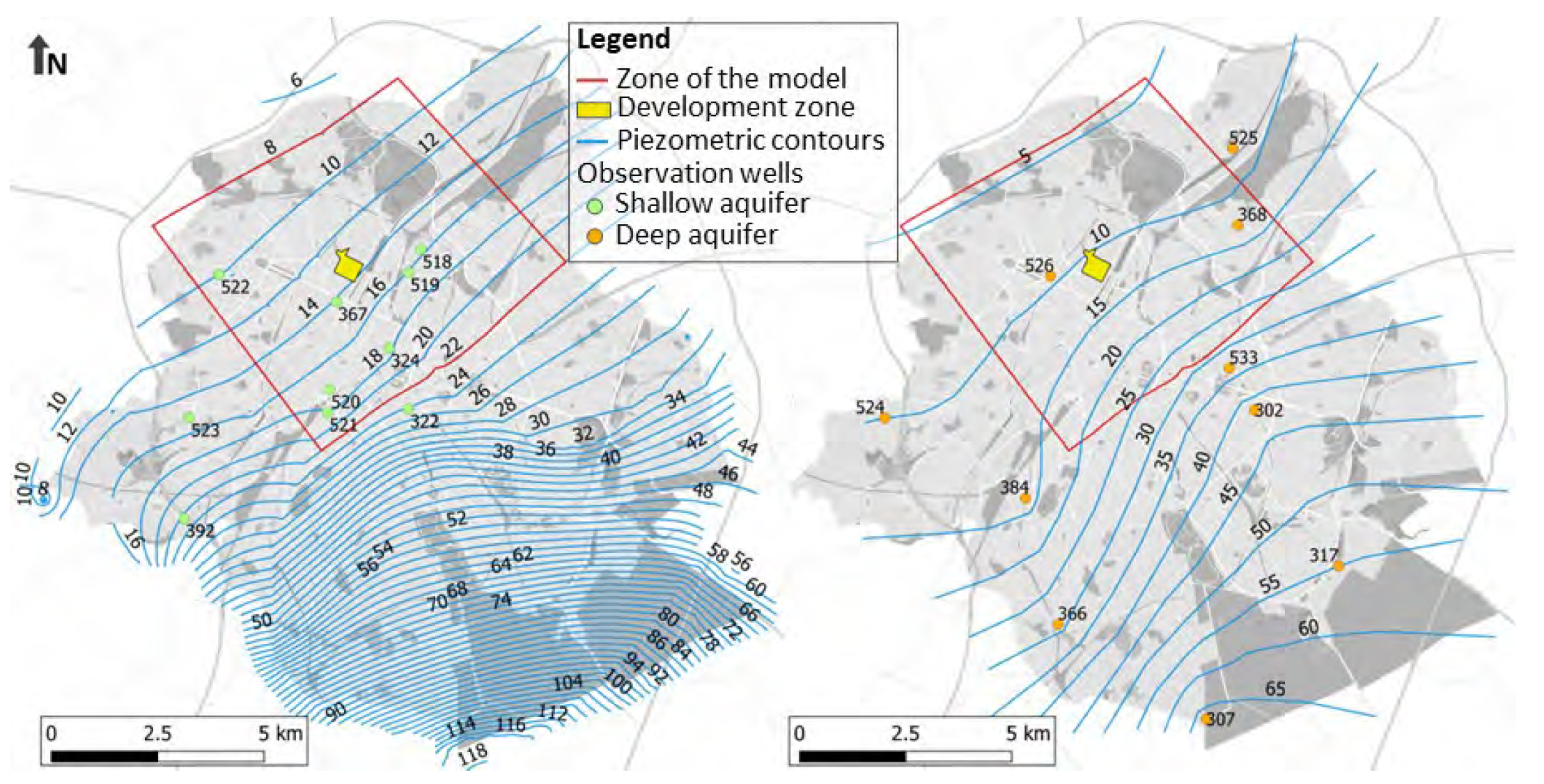
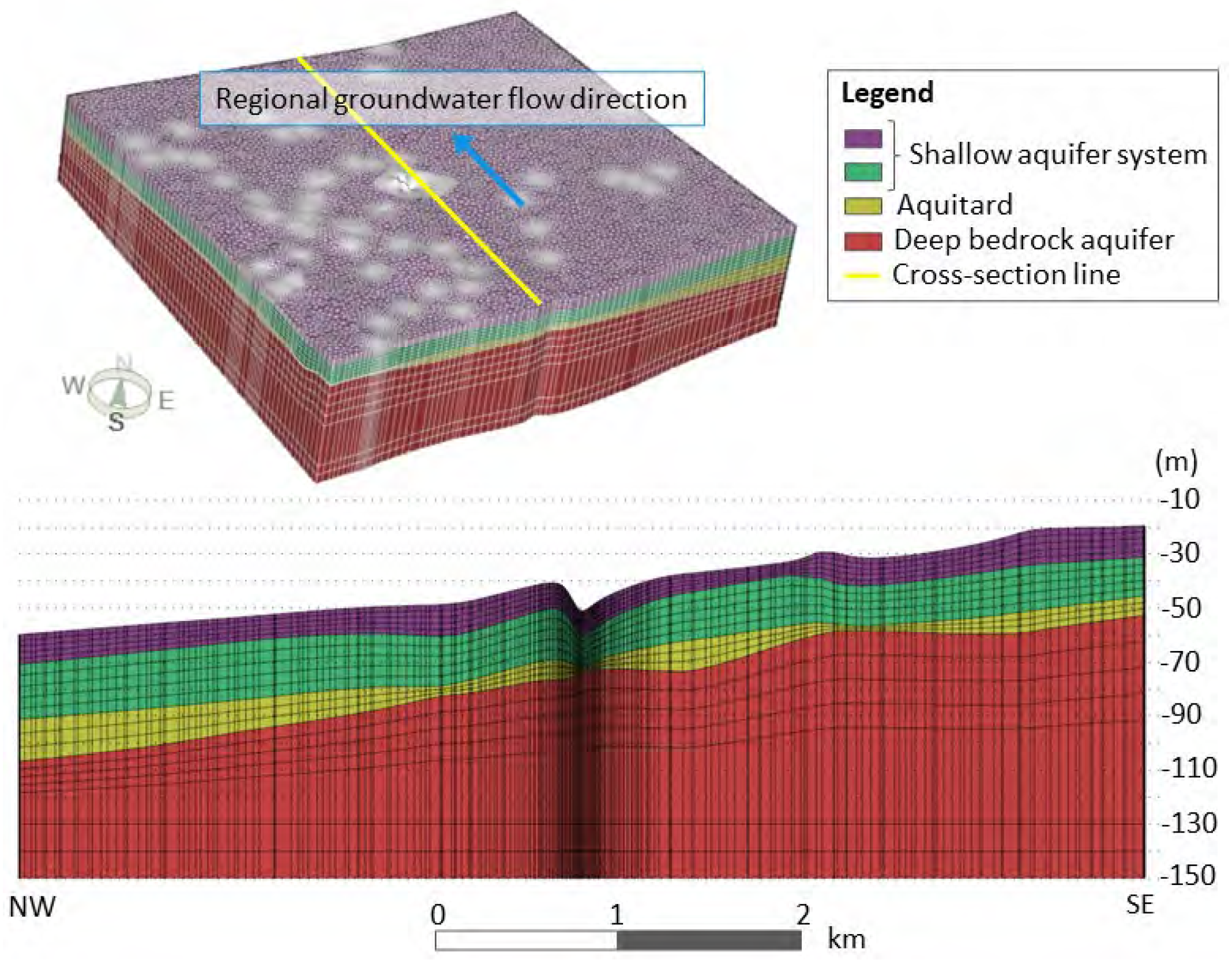
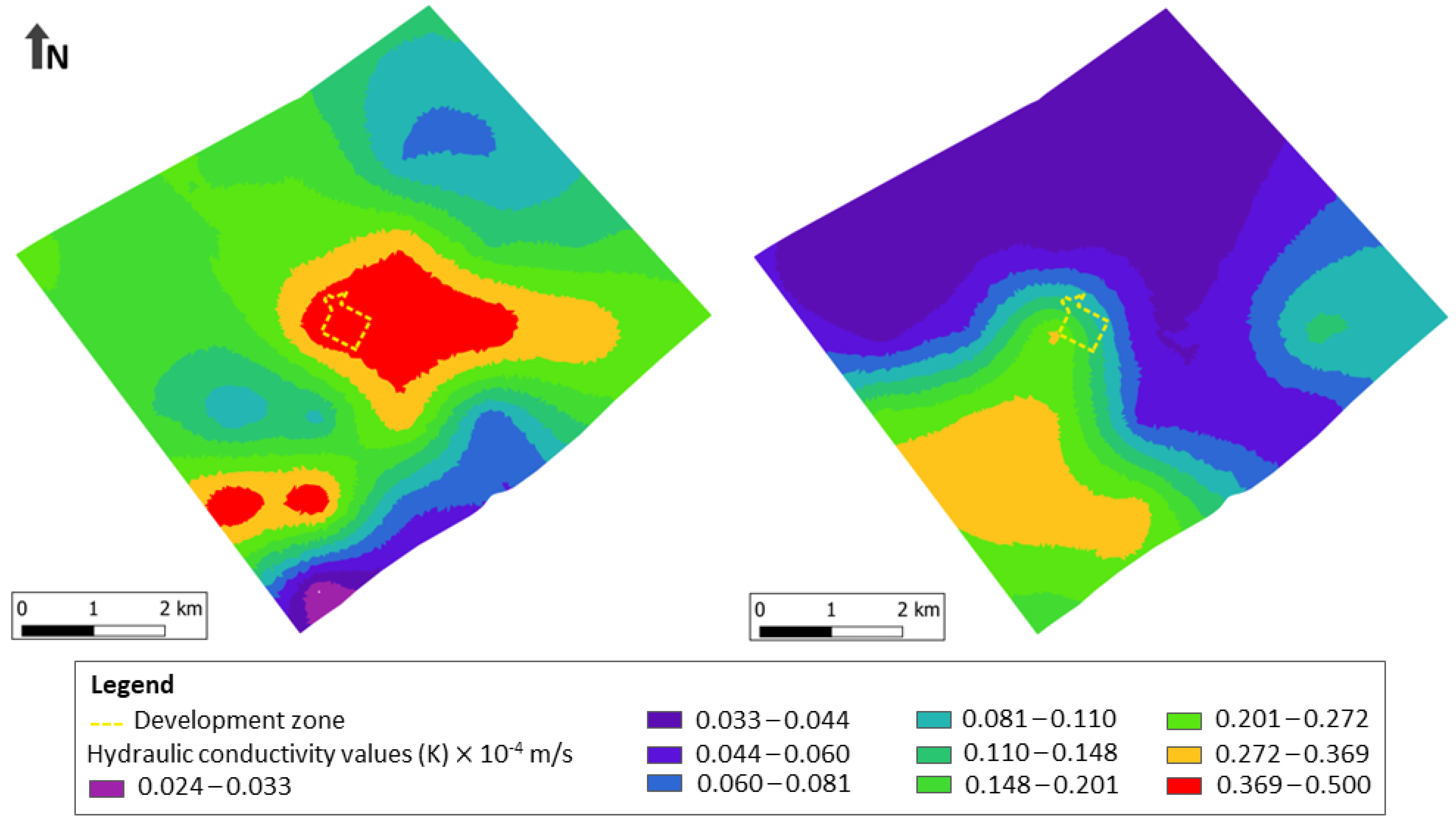
2.2.2. Hydrogeology Context

The geological context has already been described in a previous paper [3] and interpreted by Devleeschouwer et al. [32]. From top to bottom, it consists of Cenozoic loose sediments overlying Mesozoic Cretaceous marl and chalk, and at depth, there is Paleozoic bedrock consisting of fractured phyllites and quartzites. To summarize, a ‘shallow aquifer’ can be considered to consist of a succession of sand and clayey deposits. This aquifer system overlies an Upper Paleocene clay layer located at a depth of 74 m and of about 10 m thickness [33]. This clay layer lies directly on the Cretaceous layers reduced to 9 m of thickness with marl (above) and chalk (below). Under these Cretaceous formations, the Paleozoic fractured bedrock is considered the ‘deep aquifer’ system.

A simplified map showing the model boundaries (see Section 2.3.2, the available piezometers, and the three ATES systems is shown in Figure 2. Two ATES systems (Building 1 and Building 2) (Figure 1) are exploiting the shallow aquifer system with the sandy portions acting as aquifers and hosting the well screens. The third ATES system has wells screened in the deep aquifer made of fractured phyllites and quartzites. The low permeability layers between these two aquifers (i.e., the clay layer of the Upper Paleocene and the Cretaceous marls) separate the shallow aquifer system from this deep aquifer.

The potentiometric behaviors in these two aquifer systems are different, as shown on the regional potentiometric maps (Figure 2) [33]. Pumping tests performed in the upper aquifer system have shown no measurable influence on the Paleozoic bedrock aquifer system [3].

2.3. Methods

2.3.1. Groundwater Flow and Heat Transport Equations

The heat transport equation in a saturated porous medium can be written as [1,2]:

$$\frac{\partial {\rho }_b{c}_{b}T}{\partial t}=-\nabla \cdot \left[{\rho }_w{c}_w\mathit{q}T-{\lambda }_b\nabla T\right]+Q_T$$

(1)

where ∇T is the temperature gradient (°K/m), the main variable is the temperature $T$ (°K) and the main properties or parameters influencing this transport are the bulk thermal conductivity ${\lambda }_b$ (W/(m°K)) and heat capacity $c_b$ (J/(kg°K)) of the porous medium. The other properties are linked to groundwater with the density ${\rho }_w$ (kg/m³) and heat capacity $c_w$ (J/(kg°K)). The groundwater flux vector $\mathit{q}$ (m/s) is obtained from Darcy’s law. External heat or sink sources are taken into account through a positive or negative value of $Q_T$ (W/m³), respectively.

The groundwater flow is solved by taking into account the pumping and reinjection influences using the following transient equation in saturated conditions [1,2]:

$$\nabla \cdot {\rho }_w\left(\mathit{K}\cdot \nabla h\right)+{\rho }_w{q}^{\prime }={\rho }_w{S}_s\frac{\partial h}{\partial t}$$

(2)

where the main variable is the potentiometric $h$ (m), $\nabla h$ is the piezometric gradient vector (-), and the main properties or parameters influencing this groundwater flow are the hydraulic conductivity tensor $\mathit{K}$ (m/s), and the specific storage coefficient $S_s$ (m⁻¹). Pumping and reinjection are taken into account through the negative and positive values of $q^{\prime }$ (s⁻¹), respectively.

Feflow^® allows solving the groundwater flow problem in saturated or variably saturated conditions, coupled with heat transport with temperature-dependent groundwater density and viscosity. This software allows very flexible meshes of finite elements.

To link the groundwater pumping and reinjection to the thermal energy needs, we use the following expression of the power P (in W) [1,2]:

$$P=\frac{Q\mathsf{∆}T{\rho }_w{c}_w}{\left(1-\frac{1}{COP}\right)}$$

(3)

where the coefficient of performance COP (-) of the heat pump can be expressed as the ratio between the geothermally produced and the total required work. This equation shows that this thermal energy is indeed directly proportional to the water flow rate Q (m³/s) and the temperature difference ∆T (°K).

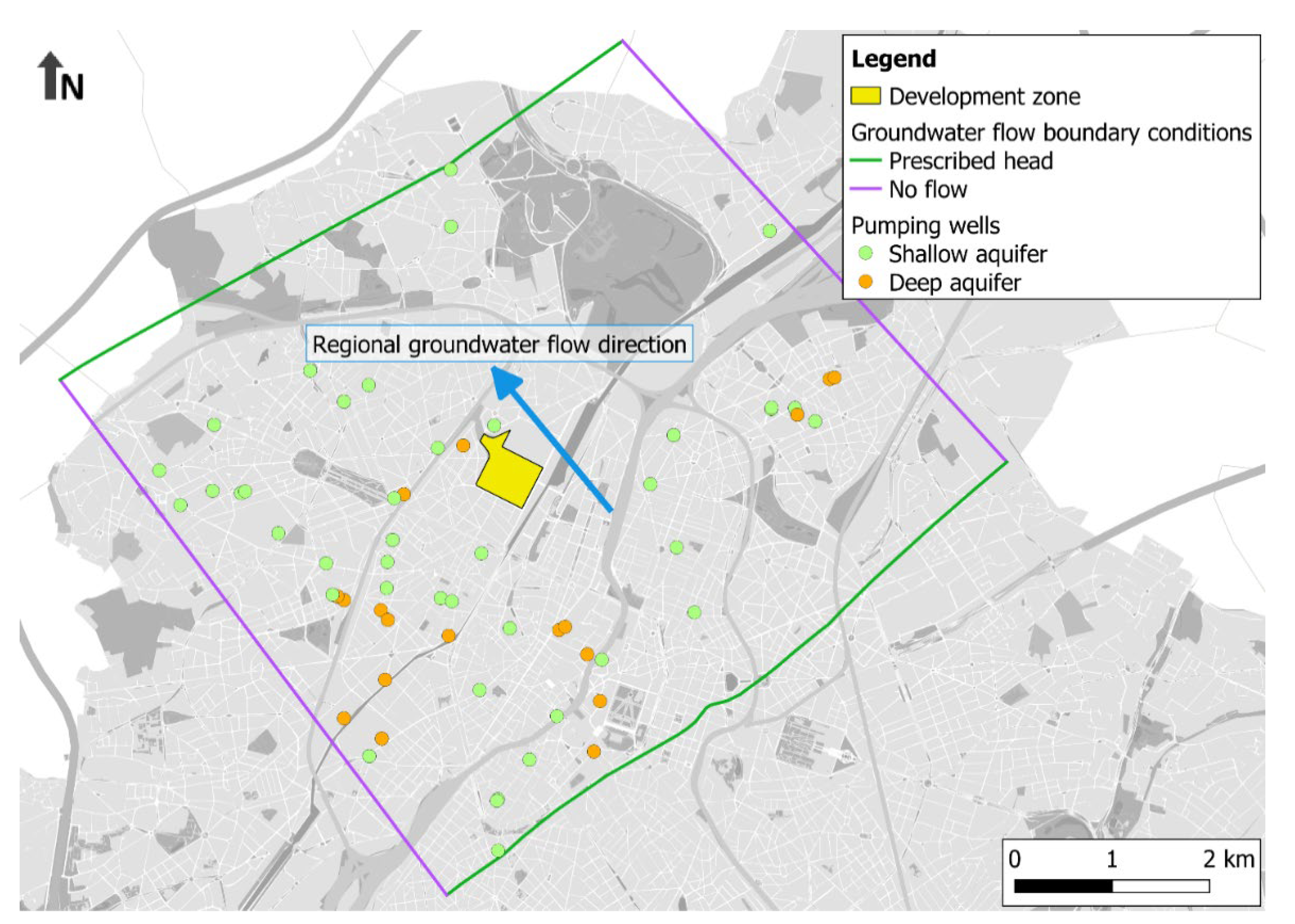
2.3.2. Conceptualization

A total of 20 layers were discretized in the 3D model. From the top, ten layers represent the shallow confined Cenozoic aquifer system: the first 5 layers correspond to the top part of the upper aquifer, layers 6 and 7 are used for a clayey part, and layers 8–10 for the lower aquifer sandy part of these Cenozoic sediments. Three layers are used to represent the aquitard consisting of the clay layer at the bottom of the Cenozoic sediments, the Cretaceous marls, and the Cretaceous chalks of low hydraulic conductivity. Then, seven layers represent the fractured Paleozoic bedrock until a depth of 150 m: five layers in the upper fractured zone, and two layers in the less fractured and less permeable zone. The bottom of the model is arbitrarily set at an altitude of −150 m (i.e., a depth of about 170 m) where relatively low permeability is observed (by pumping tests) and because the screens of the deep ATES system (Building 3) are located at an altitude between −67 m and −138 m (Figure 3). The groundwater flow is simulated in 3D including vertical and horizontal flow components (cfr Section 3.1). Feflow© allows to simulate the effect of temperature changes on the groundwater density and viscosity. However, constant hydraulic conductivity values have been adopted as the variation can be neglected for limited changes in temperature.

The boundaries and boundary conditions (BCs) were chosen according to regional hydrogeological data [33]. The top of the model corresponds to a no-flow BC, which is induced by the low permeability of the overlying confining layers and the largely urbanized land surface. As mentioned previously, the bottom boundary is set at a depth of 150 m with a no-flow BC as at this depth, the bedrock is less permeable [34] and the vertical component of the flow can be neglected. The lateral boundaries were chosen at a ‘large enough’ distance compared with the radius of influence as interpreted from local pumping tests. On the SE and NW lateral boundaries (Figure 4), potentiometric heads are prescribed along head contour lines in the shallow aquifer and based on interpolated heads from the potentiometric map in the bedrock aquifer [33]. No flux BCs were chosen on the NE and SW lateral boundaries (Figure 4) as they are globally parallel to the general groundwater flow directions, as well in the shallow aquifer and also in the deep aquifer. All the ATES pumping and injection wells and other water production wells are represented by prescribed fluxes (i.e., depth-averaged distributed onto different layers if different layers are screened in the borehole) on the corresponding nodes of the finite element mesh.

In the development zone (in yellow in Figure 4), the size of the finite element can be very small, from a few cm near the wells to a few tens of meters near the boundaries of this area of interest. In total, the 3D model consists of 1,248,420 finite elements with 20 layers of 62,421 elements. Specifically, in the development zone (area of interest), the finite element mesh refinement leads to a total number of finite elements of 434,520.

For the heat transport BCs, a temperature of 12.4 °C was chosen along the lateral boundaries. This temperature is the natural background temperature. A zero heat flux is assumed on the top as on the bottom of the model. This means that the air temperature influence and the mean deep geothermal energy flux are neglected [3,35].

As a first step, a steady-state groundwater flow was calculated from the initial potentiometric conditions. Then, the calculated steady-state potentiometric map was used for starting the transient groundwater flow. For heat transport, the natural background temperature was chosen as the initial temperature in the whole model.

3. Results

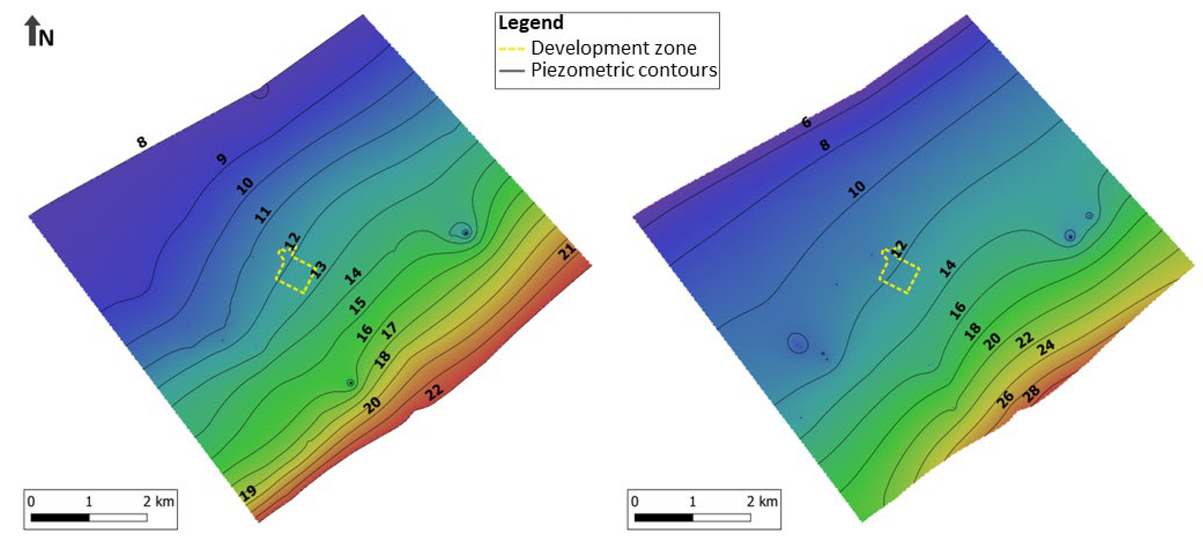
3.1. Groundwater Flow Simulations

First, the model was calibrated for groundwater flow in steady state conditions on the observed potentiometric situation of 1 March 2013. Parameter values were adjusted manually in order to obtain calculated heads as close as possible to observed potentiometric heads in both aquifers. Then, an automatic calibration using PEST [36] and associated with 30 pilot points [37] was performed. This procedure allowed us to obtain a detailed spatial distribution of the optimized hydraulic conductivity values in the model (Figure 5). Essentially, the hydraulic conductivity values of the aquifers were optimized using this procedure. For the low permeability zone forming the aquitard, horizontal hydraulic conductivity values of 1 × 10⁻⁷ m/s and 1 × 10⁻⁸ m/s were chosen for the Cretaceous base deposits and for the Cenozoic clayey layer, respectively, and a ratio $K_h/K_v=10$ was adopted between the horizontal and vertical hydraulic conductivities. This calibration generated a RMSE (Root Mean Square Error) of 1.02 × 10⁻⁶ m. The standard deviation is 1.08 × 10⁻⁶ m and residuals are of the order of 10⁻⁷ to 10⁻⁶ m. This calibration appears to be ideal; however, it should be noted that if we had more measured data (i.e., additional potentiometric data in the shallow as in the deep aquifers) it could be considered as much more robust. Simulated potentiometric maps for the situation on 1 March 2013 (before starting the Building 1 ATES system) are given in Figure 6.

Then the steady state situation is used as the initial potentiometric map for a transient state calibration that consists of fitting the values of the storage coefficient to reproduce the time variability of the potentiometric heads as it was observed in previous pumping tests in the shallow and bedrock aquifers [3,38]. The detailed results of this calibration, as described by De Paoli [38], highlight the major fact that the pumping by Building 3 in the lower aquifer has only very limited effect (maximum 5 to 20 cm drawdown) on the potentiometric (observed and simulated) map in the shallow aquifer (i.e., where Buildings 1 and 2 have their ATES systems).

3.2. Heat Transport Simulations

In this section, the main results of the heat transport simulations are summarized from the work of De Paoli [38]. Different scenarios were previously discussed involving the ATES systems in Buildings 1 and 2, and their respective interactions [3]. Indeed, the power extracted for each system is approximated based on the measured abstraction rates and prescribing a ΔT of 6 °K between the pumping and reinjection temperatures [3] (

Table 1. Mean power extraction by the different ATES systems in Buildings 1, 2 and 3 and the associated assumed ΔT.

	Power (kW)		ΔT (°C)	Number of Doublets
	Heating (1 October to 31 March)	Cooling (1 April to 30 September)
Building 1	44	86	6	4
Building 2	82	79	6	4
Building 3	286	285	Tinj cst (7 and 18)	5

). In reality, these last values are not well known as the heat pump input and output water temperatures are influenced by the temperature in the building basements and by actual frequent switches between pumping and injection as imposed by the temperature optimization in each building. Over years, a clear imbalance is observed seasonally in the demand for Building 1. In contrast, the power demand for Building 2 seems balanced (Table 1) [3]. Next, the ATES in Building 3 tapping the deep aquifer is added. Indeed, the mean power can be multiplied by the duration of each period (6 months) to find the total heating or cooling energy consumed by each building. For example, the ATES of Building 3 uses about 1250 MWh during one season. The time steps of the heat transport simulations can vary from about 1 s until 15 days. Very short time steps are automatically chosen by the software Feflow© when required for numerical stability and convergence needs.

3.2.1. Scenario Descriptions

The reference scenario (scenario 1) reproduces as far as possible the actual situation as known from the different available data for the three ATES systems. The ATES in Building 1 started operation on 1 March 2014, the ATES in Building 2 started on 1 August 2017, and finally, the ATES in Building 3 started on 1 April 2020.

The operational characteristics of this last ATES are assumed as foreseen in the first feasibility study [34], leading to a mean power that is unbalanced between the heating and cooling seasons (Table 1). Here, however, the injection temperatures are assumed constant at 7 °C and 18 °C for the heating and cooling operations, respectively [34]. Each doublet is assumed to contribute equally (1/5) to the total needed flow rate.

Other different scenarios can be considered for the heat transport simulations. A second scenario is considered with a 50% increase in the cooling needs in Building 3. The third scenario corresponds to a constant ΔT equal to 6 °C for the ATES in Building 3. Scenarios 4 and 5 consider increased values of thermal conductivity (up to 3 W/m °K) and hydraulic conductivity (from 1 × 10⁻⁷ to 4 × 10⁻⁷ m/s), respectively, in the main aquitard between the shallow and the deep aquifers. However, the results for those last scenarios will not be commented on here as no significant changes in the simulated heat plumes and heat interactions were simulated.

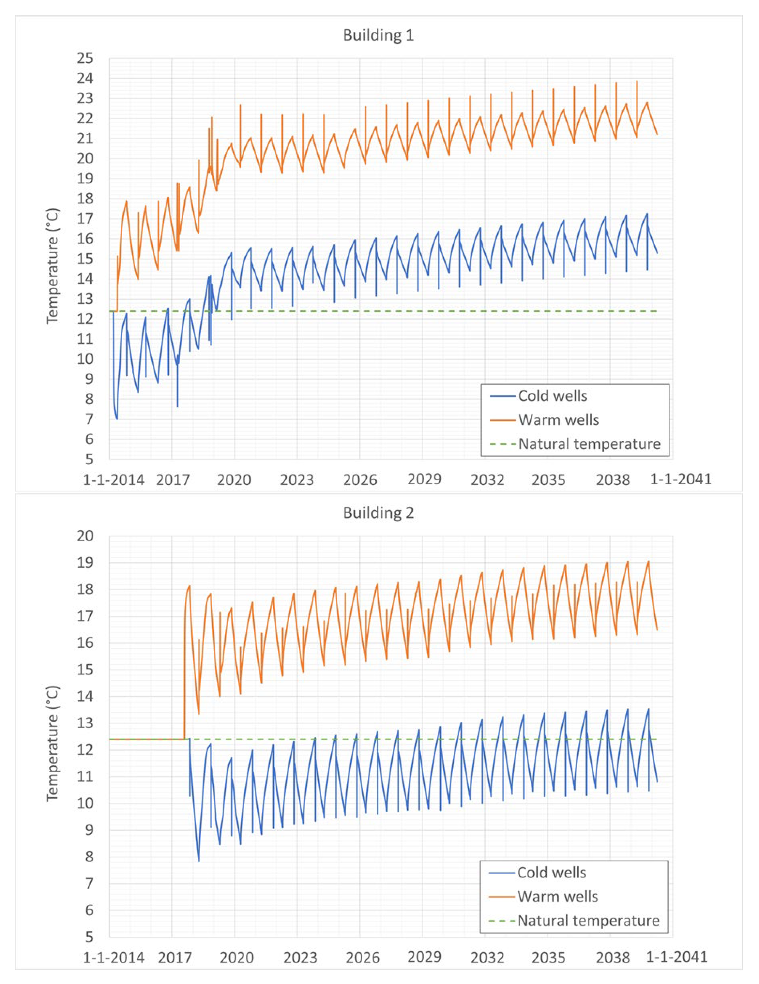
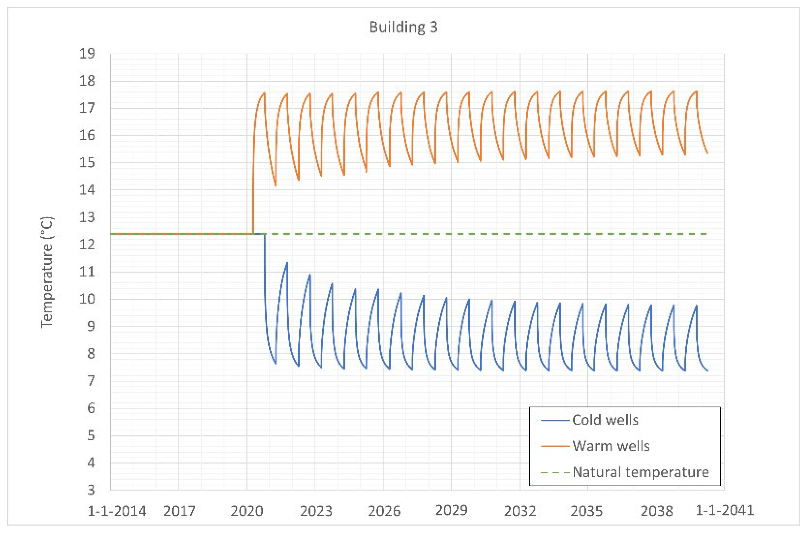
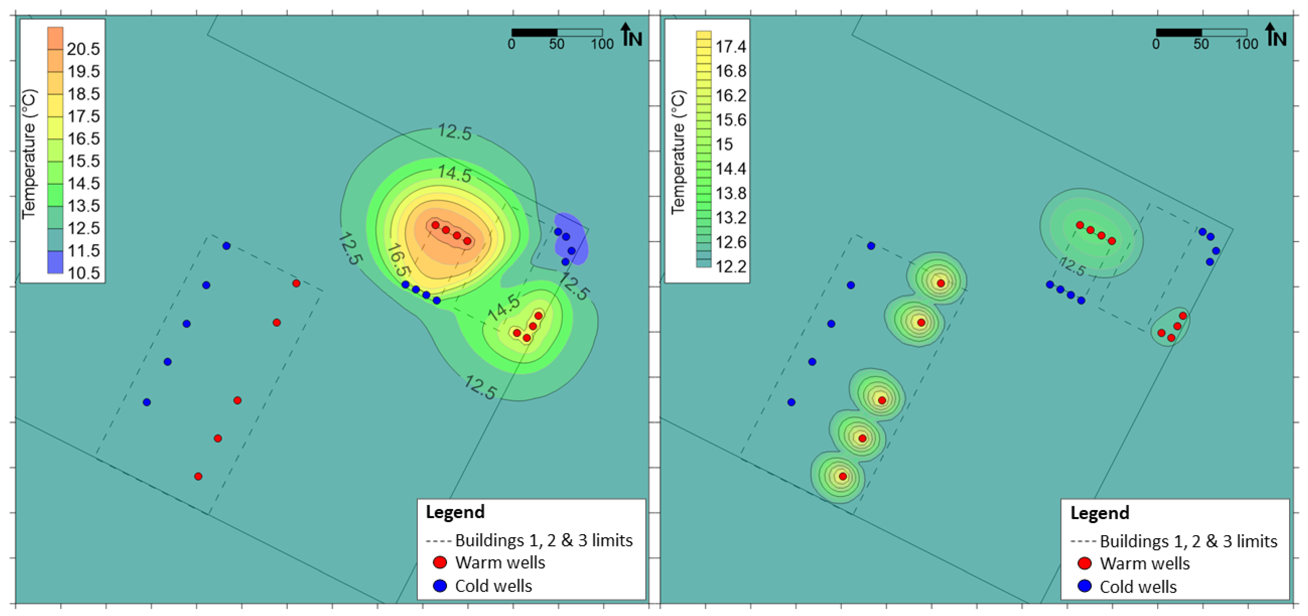
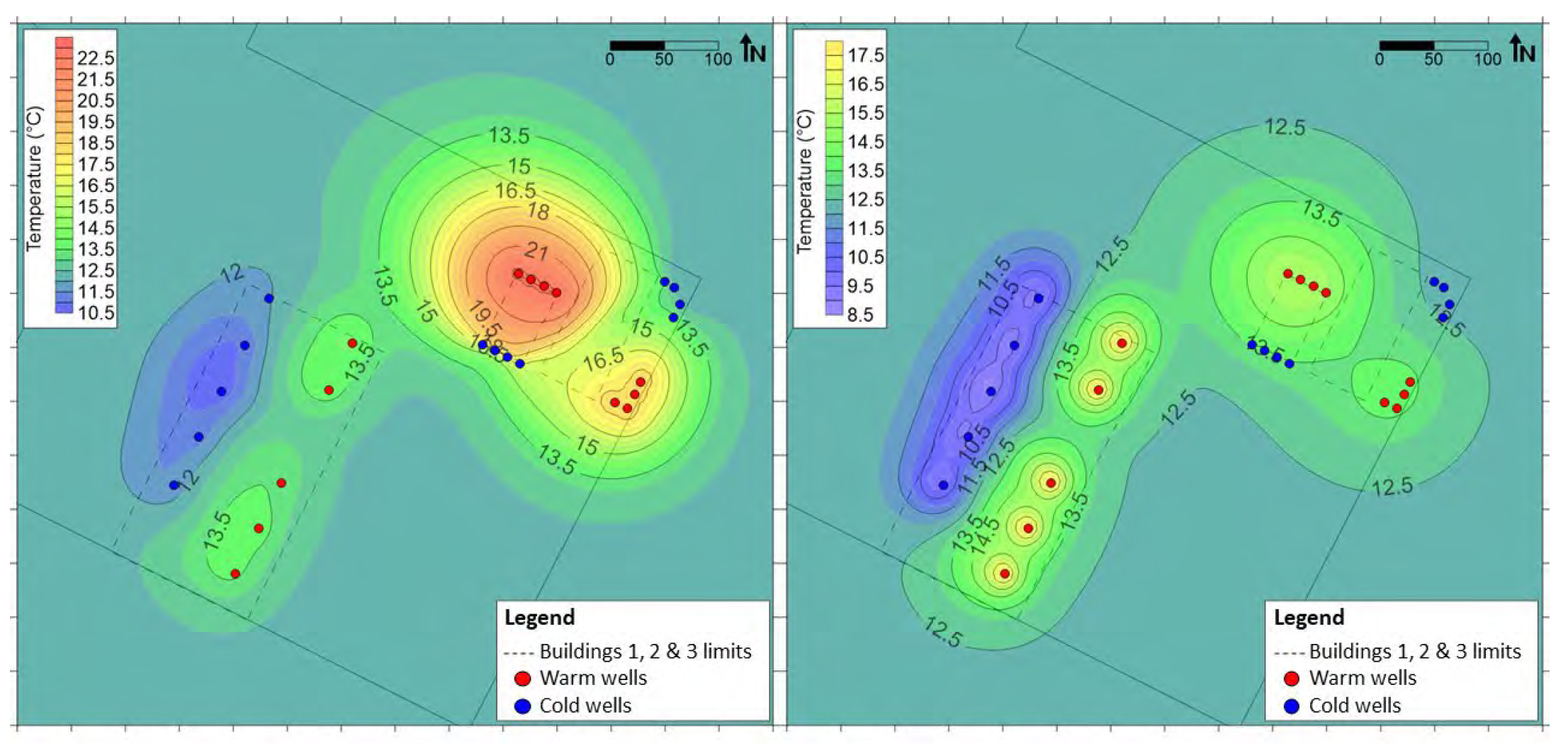
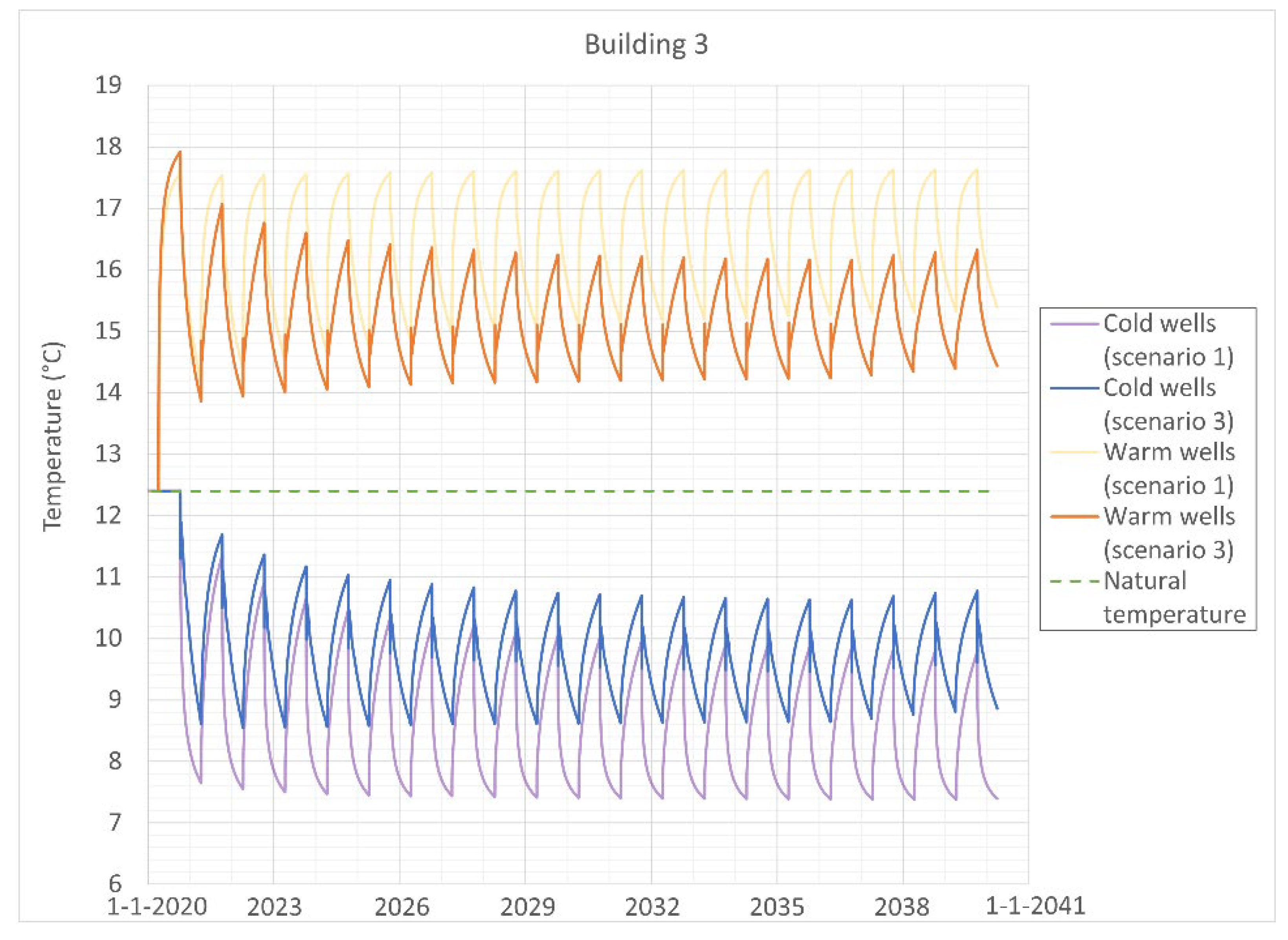
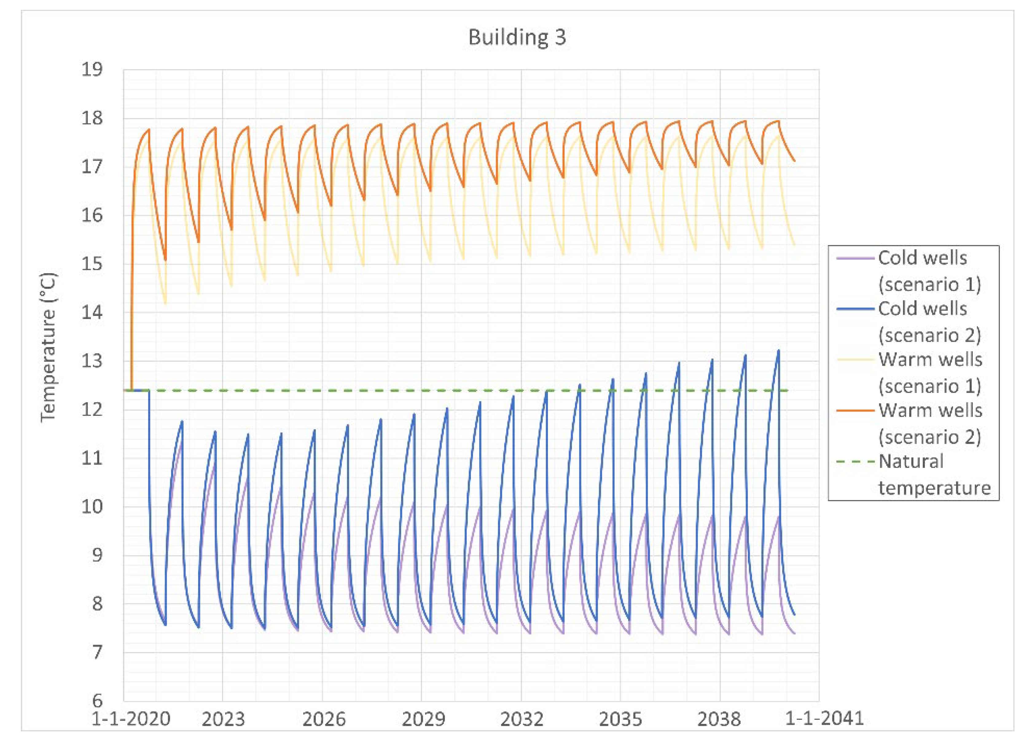
3.2.2. Scenario Simulation Results

Ongoing and future conditions for the three ATES systems are calculated from 1 January 2014 until 31 March 2040, with no evolution in time of the power used for heating or cooling. For scenario 1 (reference scenario), the temperature increases year after year in the warm (WW) and in the cold wells (CW) of Buildings 1 and 2 (Figure 7). As commented by Bulté et al. [3]: ‘a step increase was simulated in the hot wells at each spring period corresponding to the start of each building cooling period and thus to injection of hot water in the hot wells’. The simulated temperature increases systematically during the whole summer period in the hot wells. This is also the case in the cold pumping wells, and after 2016, the coldest spring temperatures continued to shift higher and thus continued to rise during the summer. As indicated previously [3], the Building 1 imbalance (i.e., requiring less energy for heating than cooling), is causing this trend for both Buildings 1 and 2. A step temperature decrease is also simulated in the cold injection wells at the beginning of the winter, and the temperature decreased during the whole period. Then, the temperature also decreases slightly near the hot wells but never reaches back to the initial natural temperature. In the long term, the coldest simulated temperatures that can be found at the beginning of the summer period in the hot wells continue to increase each year from 12.4 and reach 21 °C in 2039.

For Building 3, starting from the initial 12.4 °C in the deep aquifer, the simulated evolution of the mean temperature in the hot and cold wells does not show any trend (Figure 8). This results from the well-balanced power needs for heating and cooling combined with the limited influence of the shallow aquifer changes on the deep aquifer conditions. This is indeed very positive for the current and future efficiency of the ATES.

Simulated heat and cold plumes in the shallow aquifer show the negative thermal interferences between the heat plume and the cold wells of the Building 1 and 2 systems (Figure 9) and the progressive temperature increase in the cold wells. Consequently, in this aquifer, the cold storage becomes less efficient year after year. In the deep aquifer, heat plumes are logically seen around the hot wells at the end of the summer. Slight heat plumes are also simulated in this aquifer and are located just below the hot wells of Buildings 1 and 2 in the upper aquifer. This shows that the hot plumes in the shallow aquifer induce only a limited influence on the deep aquifer.

The heat and cold plumes are simulated for more than 20 years for operation with the power use maintained at current levels (Figure 10). On 1 October 2039, it appears that the large heat plume generated in the upper aquifer (Figure 10, left) does not impact the cold wells in the deep aquifer (Figure 10, right). From the reverse perspective, the hot and cold plumes generated in the deep aquifer by the ATES system of Building 3 do not have a significant effect on the shallow aquifer and hot and cold wells of Buildings 1 and 2.

However, as expected, in the shallow aquifer, the cold wells of Building 1 and to a lesser extent also those of Building 2, are affected by the large heat plume from the hot wells of Building 1.

For the second scenario involving a 50% increase in the cooling needs in Building 3, the simulated evolution of the mean temperature at the hot and cold wells (Figure 11) can be compared with those of the reference scenario. Logically, we observe that the simulated temperature variation in the hot wells decreases each year so that in 2039, this variation is less than 1 °C between 1 April and 1 October. In contrast, in the cold wells, a higher temperature variation is calculated each year, adding to a general trend towards higher temperatures induced by the thermal imbalance. In 2039, the temperature varies between 7.6 and 13.1 °C, resulting in a temperature higher than the natural background of 12.4 °C at the end of the summer period. Indeed, the efficiency of the cooling should be slightly decreased accordingly, but this temperature increase is remarkably slow and weak, showing a general high thermal inertia of the deep aquifer in relation to a highly imbalanced ATES system. However, a constant injection temperature may also contribute to this slow increase.

Scenario 3 with a constant ΔT equal to 6 °C for the ATES in Building 3, induces a slight temperature increase in the long term (i.e., after more than 17 years) in the wells of the Building 1 ATES system and also a slight temperature decrease in those of the Building 2 ATES system. This influence is, however, very weak. Conversely, scenario 3 induces a clear change in the temperature variations observed in the hot and cold wells of Building 3, with lower temperatures and lower variations in the hot wells and higher temperatures and lower variations in the cold wells (Figure 12). Yearly, the mean temperature is stabilized, as for the reference scenario, but globally, the ATES system is slightly less efficient. Therefore, an operational scheme giving priority to maintaining a constant ΔT is not specifically recommended.

4. Discussion and Conclusions

As shown previously [3], for Building 1, a large thermal imbalance providing more hot water than cold water to the shallow aquifer led to negative interferences between the heat plume in the aquifer and the cold wells. For this building, urgent corrections must be implemented in the energy operational strategy (e.g., increased use of heat during the winter period, increased night ventilation, and increased window solar protection) [3]. In the shallow aquifer, the general increase in temperatures induced by this imbalance affects the efficiency of the ATES system of Building 2. Year after year, the growing heat plumes are not sufficiently dispersed or diluted by the natural groundwater flow in the aquifer.

Following the feasibility study [34], the third ATES system located in the deep aquifer has well-balanced annual heat and cold power. Consequently, the simulated evolution of the mean temperature at the hot and cold wells does not show any trend. Simulated heat and cold plumes are seen around the hot and cold wells, respectively, at the end of the cooling and heating seasons, as is logically expected.

Interactions between the systems of Buildings 1 and 2 in the shallow aquifer and the system of Building 3 in the deep aquifer are limited. However, in the mid- and long-term, heat and cold exchanges can be seen through the simulated heat and cold plumes that are induced by the ATES systems located in the other aquifer. Those simulated interactions remain very limited and have no important consequences on the efficiencies of the systems.

The ATES system of Building 3 seems very robust and stable. Even if this system evolves towards a strongly imbalanced scheme with a cooling power that becomes double the heating power (scenario 2), the efficiency of the cooling would only be slightly decreased after 20 years, with a temperature in the deep aquifer (13.1 °C) higher than the natural background (12.4 °C). Maintaining a constant ΔT between the warm and cold wells does not significantly change the impact or the efficiency.

More generally, the seasonal heat storage in these two aquifers separated by an aquitard composed of the weathered top of the bedrock, the overlying low permeability Cretaceous base deposits, and a Cenozoic clayey layer is a success story. The only weak point is the effect of the recurrent imbalance of the cooling and heating needs in Building 1. This induces a clear impact on the upper aquifer temperature, and consequently, on the mid-and long-term efficiencies for both ATES systems located in this aquifer (Buildings 1 and 2).

However, as usual, the reliability of such models is closely linked to the availability of measured potentiometric heads, groundwater temperatures, and detailed pumping and injection data. In this particular case, and specifically viewing the simulated trend in the upper aquifer, the acquisition of such measured data is crucial to improve the robustness of the model results (i.e., with more detailed and long calibration periods). Real estate developers, designers, and builders should give more attention to these needs in feasibility studies as well as in their ‘after sales services’.

References

1. Dassargues, A. Hydrogeology—Groundwater Science and Engineering; Taylor & Francis CRC Press: Boca Raton, FL, USA, 2018; pp. 323–343. [Google Scholar]
2. Dassargues, A. Hydrogéologie Appliquée—Science et Ingéniérie des Eaux Souterraines; Dunod: Paris, France, 2020; pp. 341–364. (In French) [Google Scholar]
3. Bulté, M.; Duren, T.; Bouhon, O.; Petitclerc, E.; Agniel, M.; Dassargues, A. Numerical modeling of the interference of thermally unbalanced Aquifer Thermal Energy Storage systems in Brussels (Belgium). Energies 2021, 14, 6241. [Google Scholar] [CrossRef]
4. Yapparova, A.; Matthäi, S.; Driesner, T. Realistic simulation of an aquifer thermal energy storage: Effects of injection temperature, well placement and groundwater flow. Energy 2014, 76, 1011–1018. [Google Scholar] [CrossRef]
5. Lee, K.S. Effects of regional groundwater flow on the performance of an aquifer thermal energy storage system under continuous operation. Hydrogeol. J. 2014, 22, 251–262. [Google Scholar] [CrossRef]
6. Bloemendal, M.; Hartog, N. Analysis of the impact of storage conditions on the thermal recovery efficiency of low-temperature ATES systems. Geothermics 2018, 71, 306–319. [Google Scholar] [CrossRef]
7. Bloemendal, M.; Olsthoorn, T. ATES systems in aquifers with high ambient groundwater flow velocity. Geothermics 2018, 75, 81–92. [Google Scholar] [CrossRef]
8. Gao, L.; Zhao, J.; An, Q.; Wang, J.; Liu, X. A review on system performance studies of aquifer thermal energy storage. Energy Procedia 2017, 142, 3537–3545. [Google Scholar] [CrossRef]
9. Fleuchaus, P.; Godschalk, B.; Stober, I.; Blum, P. Worldwide application of aquifer thermal energy storage—A review. Renew. Sustain. Energy Rev. 2018, 94, 861–876. [Google Scholar] [CrossRef]
10. Hamada, Y.; Marutani, K.; Nakamura, M.; Nagasaka, S.; Ochifuji, K.; Fuchigami, S.; Yokoyama, S. Study on underground thermal characteristics by using digital national land information, and its application for energy utilization. Appl. Energy 2002, 72, 659–675. [Google Scholar] [CrossRef]
11. Lo Russo, S.; Civita, M.V. Open-loop groundwater heat pumps development for large buildings: A case study. Geothermics 2009, 38, 335–345. [Google Scholar] [CrossRef]
12. Andrews, C. The impact of the use of heat pumps on ground-water temperatures. Ground Water 1978, 16, 437–443. [Google Scholar] [CrossRef]
13. Molina-Giraldo, N.; Bayer, P.; Blum, P. Evaluating the influence of thermal dispersion on temperature plumes from geothermal systems using analytical solutions. Int. J. Therm. Sci. 2011, 50, 1223–1231. [Google Scholar] [CrossRef]
14. Ma, R.; Zheng, C. Effects of density and viscosity in modeling heat as a groundwater tracer. Ground Water 2010, 48, 380–389. [Google Scholar] [CrossRef] [PubMed]
15. Wildemeersch, S.; Jamin, P.; Orban, P.; Hermans, T.; Klepikova, M.; Nguyen, F.; Brouyère, S.; Dassargues, A. Coupling heat and chemical tracer experiments for estimating heat transfer parameters in shallow alluvial aquifers. J. Contam. Hydrol. 2014, 169, 90–99. [Google Scholar] [CrossRef]
16. Wagner, V.; Li, T.; Bayer, P.; Leven, C.; Dietrich, P.; Blum, P. Thermal tracer testing in a sedimentary aquifer: Field experiment (Lauswiesen, Germany) and numerical simulation. Hydrogeol. J. 2014, 22, 175–187. [Google Scholar] [CrossRef]
17. Hermans, T.; Wildemeersch, S.; Jamin, P.; Orban, P.; Brouyère, S.; Dassargues, A.; Nguyen, F. Quantitative temperature monitoring of a heat tracing experiment using cross-borehole ERT. Geothermics 2015, 53, 14–26. [Google Scholar] [CrossRef] [Green Version]
18. Casasso, A.; Sethi, R. Modelling thermal recycling occurring in groundwater heat pumps (GWHPs). Renew. Energy 2015, 77, 86–93. [Google Scholar] [CrossRef] [Green Version]
19. Lo Russo, S.; Taddia, G.; Cerino Abdin, E.; Verda, V. Effects of different re-injection systems on the thermal affected zone (TAZ) modelling for open-loop groundwater heat pumps (GWHPs). Environ. Earth Sci. 2016, 75, 1–14. [Google Scholar] [CrossRef]
20. Klepikova, M.; Wildemeersch, S.; Jamin, P.; Orban, P.; Hermans, T.; Nguyen, F.; Brouyère, S.; Dassargues, A. Heat tracer test in an alluvial aquifer: Field experiment and inverse modelling. J. Hydrol. 2016, 540, 812–823. [Google Scholar] [CrossRef] [Green Version]
21. Hermans, T.; Nguyen, F.; Klepikova, M.; Dassargues, A.; Caers, J. Uncertainty quantification of medium-term heat storage from short-term geophysical experiments. Water Resour. Res. 2018, 54, 2931–2948. [Google Scholar] [CrossRef] [Green Version]
22. Wang, G.; Song, X.; Shi, Y.; Sun, B.; Zheng, R.; Li, J.; Pei, Z.; Song, H. Numerical investigation on heat extraction performance of an open loop geothermal system in a single well. Geothermics 2019, 80, 170–184. [Google Scholar] [CrossRef]
23. Park, D.K.; Kaown, D.; Lee, K.K. Development of a simulation-optimization model for sustainable operation of groundwater heat pump system. Renew. Energy 2020, 145, 585–595. [Google Scholar] [CrossRef]
24. Sommer, W.; Valstar, J.; Leusbrock, I.; Grotenhuis, T.; Rijnaarts, H. Optimization and spatial pattern of large-scale aquifer thermal energy storage. Appl. Energy 2015, 137, 322–337. [Google Scholar] [CrossRef]
25. Bakr, M.; van Oostrom, N.; Sommer, W. Efficiency of and interference among multiple Aquifer Thermal Energy Storage systems; A Dutch case study. Renew. Energy 2013, 60, 53–62. [Google Scholar] [CrossRef]
26. Vanhoudt, D.; Desmedt, J.; Van Bael, J.; Robeyn, N.; Hoes, H. An aquifer thermal storage system in a Belgian hospital: Long-term experimental evaluation of energy and cost savings. Energy Build. 2011, 43, 3657–3665. [Google Scholar] [CrossRef]
27. Kranz, S.; Frick, S. Efficient cooling energy supply with aquifer thermal energy storages. Appl. Energy 2013, 109, 321–327. [Google Scholar] [CrossRef]
28. Bloemendal, M.; Olsthoorn, T.; Boons, F. How to achieve optimal and sustainable use of the subsurface for Aquifer Thermal Energy Storage. Energy Policy 2014, 66, 104–114. [Google Scholar] [CrossRef]
29. Fleuchaus, P.; Schüppler, S.; Godschalk, B.; Bakema, G.; Blum, P. Performance analysis of Aquifer Thermal Energy Storage (ATES). Renew. Energy 2020, 146, 1536–1548. [Google Scholar] [CrossRef]
30. Niknam, P.H.; Talluri, L.; Fiaschi, D.; Manfrida, G. Sensitivity analysis and dynamic modelling of the reinjection process in a binary cycle geothermal power plant of Larderello area. Energy 2021, 214, 118869. [Google Scholar] [CrossRef]
31. Leontidis, V.; Niknam, P.H.; Durgut, I.; Talluri, L.; Manfrida, G.; Fiaschi, D.; Akin, S.; Gainville, M. Modelling reinjection of two-phase non-condensable gases and water in geothermal wells. Appl. Therm. Eng. 2023, 223, 120018. [Google Scholar] [CrossRef]
32. Devleeschouwer, X.; Goffin, C.; Vandaele, J.; Meyvis, B. Modélisation Stratigraphique en 2D et 3D du Sous-Sol de la Région de Bruxelles-Capitale; Final report of the project BRUSTRATI3D Version 1.0.; Royal Institute of Belgium for Natural Sciences Institute (RIBNS), Belgian Geological Survey: Brussels, Belgium, 2018; Available online: https://document.environnement.brussels/opac_css/index.php?lvl=notice_display&id=10964 (accessed on 18 October 2022). (In French)
33. IBGE—Institut Bruxellois Pour la Gestion de l’Environnement. Atlas: Hydrogéologie; Brussels Environment: Brussels, Belgium, 2020; Available online: https://geodata.environnement.brussels/client/view/82645188-dd20-430c-b1d1-df829c94dc1d (accessed on 18 October 2022). (In French)
34. AGT, Adviesbureau inzake Grondwatertechnieken. Project: KWO Gare Maritime Brussel. Nota Testen KWO-bronnen: Stand van Zaken; Report 2018 10 30-MPOS-AGT1915-Nota; Adviesbureau inzake Grondwatertechnieken: Kontich, Belgium, 2018; Volume 15, p. 43. [Google Scholar]
35. Pollack, H.N.; Hurter, S.J.; Johnson, J.R. Heat flow from the earth’s interior: Analysis of the global data set. Rev. Geophys. 1993, 31, 267–280. [Google Scholar] [CrossRef]
36. Doherty, J. PEST–Model-Independent Parameter Estimation–User Manual, 5th ed; Watermark Numerical Computing; EPA: Washington, DC, USA, 2005. [Google Scholar]
37. Doherty, J. Ground water model calibration using pilot points and regularization. Ground Water 2003, 41, 170–177. [Google Scholar] [CrossRef]
38. De Paoli, C. Modélisation de L’effet Cumulé de Plusieurs Systèmes Géothermiques Ouverts Utilisant les Aquifères Peu Profonds en Zone Urbaine. Master’s Thesis, ULiège, Liège, Belgium, 2022. Available online: http://hdl.handle.net/2268.2/14560 (accessed on 30 November 2022). (In French).
Figure 1. Location map of the study case in Brussels (Belgium). Locations of the model, development zone, and the three studied buildings and their ‘cold’ and ‘warm wells’ of the ATES systems.
Applsci 13 02934 g001
Figure 2. Observation wells and regional potentiometric maps in the shallow Cenozoic-Paleocene aquifer system (left) and in the deep Paleozoic bedrock aquifer (right).
Applsci 13 02934 g002
Figure 3. 3D view of the finite element mesh and a detailed NW–SE cross-section passing through the location of Building 3 (deep ATES system).
Applsci 13 02934 g003
Figure 4. Lateral boundaries for solving the groundwater flow. Lateral BCs for heat transport are everywhere prescribed to the natural initial temperature of 12.4 °C. Blue and green dots are pumping wells in the shallow and deep aquifers respectively, and the blue arrow shows the direction of the regional groundwater flow.
Applsci 13 02934 g004
Figure 5. Spatial distribution of the hydraulic conductivity (K) values obtained by calibration in the shallow aquifer (left) and in the upper part of the fractured bedrock aquifer (right).
Applsci 13 02934 g005
Figure 6. Calibrated potentiometric maps in the shallow aquifer (left) and in the fractured bedrock aquifer (right).
Applsci 13 02934 g006
Figure 7. Simulated long-term evolution of the mean temperature in the hot and cold wells starting from the natural background temperature of groundwater around 12.4 °C for Buildings 1 (above) and 2 (below).
Applsci 13 02934 g007
Figure 8. Simulated long-term evolution of the mean temperature at the hot and cold wells for Building 3.
Applsci 13 02934 g008
Figure 9. Simulated heat and cold plumes for 1 October 2020 (end of the first cooling period of Building 3) in the shallow (left) and the deep (right) aquifer.
Applsci 13 02934 g009
Figure 10. Simulated heat and cold plumes for 1 October 2039 in the shallow (left) and in the deep (right) aquifer.
Applsci 13 02934 g010
Figure 11. Simulated long-term evolution of the mean temperature at the hot and cold wells (in the deep aquifer) for Building 3 for the second scenario involving a cooling power of 427 kW and a heating power of 286 kW, compared with the first scenario.
Applsci 13 02934 g011
Figure 12. Simulated long-term evolution of the mean temperature at the hot and cold wells (in the deep aquifer) for Building 3 for the third scenario with a constant ΔT equal to 6 °C, compared with the first scenario.
Applsci 13 02934 g012