Communication

Application of CNN Models to Detect and Classify Leakages in Water Pipelines Using Magnitude Spectra of Vibration Sound

1
School of Information and Communication Engineering, Soongsil University, Seoul 06978, Republic of Korea
2
School of Electronic Engineering, Soongsil University, Seoul 06978, Republic of Korea
*
Author to whom correspondence should be addressed.
Appl. Sci. 2023, 13(5), 2845; https://doi.org/10.3390/app13052845
Submission received: 29 December 2022 / Revised: 8 February 2023 / Accepted: 20 February 2023 / Published: 22 February 2023

Abstract

:
Conventional schemes to detect leakage in water pipes require leakage exploration experts. However, to save time and cost, demand for sensor-based leakage detection and automated classification systems is increasing. Therefore, in this study, we propose a convolutional neural network (CNN) model to detect and classify water leakage using vibration data collected by leakage detection sensors installed in water pipes. Experiment results show that the proposed CNN model achieves an F1-score of 94.82% and Matthew’s correlation coefficient of 94.47%, whereas the corresponding values for a support vector machine model are 80.99% and 79.86%, respectively. This study demonstrates the superior performance of the CNN-based leakage detection scheme with vibration sensors. This can help one to save detection time and cost incurred by skilled engineers. In addition, it is possible to develop an intelligent leak detection system based on the proposed one.

1. Introduction

Recently, with the progress of the artificial intelligence technology based on big data, the provision of public services based on information and communications technology is expanding [1]. Accordingly, technology development and pilot projects for intelligent management systems are being actively conducted in water-related industries to mitigate economic losses. Reduction in water pressure due to leakage costs additional energy and results in secondary pollution, which is estimated to cause a loss of trillions of Korean Won per year in Korea [2].
Pipelines that transport various fluids, including water, are considered critical infrastructure assets and contribute significantly to the nation’s economy. In general, pipelines that are installed across the country to provide different services crack and fail at a given rate depending on their length. Pipeline failures are typically caused by aging infrastructures and poor environmental conditions [3,4].
In particular, water pipeline facilities are buried underground. They can be damaged by various factors, such as deterioration of materials, improper use of materials and structures for piping connections, internal corrosion, traffic load, and ground movement, which can result in leaks. Therefore, in recent years, as communication technologies have progressed, smart metering technology that collects and transmits information, such as water flow, pipe network sensor, and water quality data in real-time are being developed [5,6,7]. Real-time leak detection technology is critical for developing the remote monitoring systems of water pipes. Unfortunately, detecting leaks in advance is challenging [8]. Therefore, various approaches have been developed to detect leaks in the past.
Several approaches are based on signal processing schemes. An example is a study that proposed a method for detecting and locating leaks based on vibration sensors and generalized correlation techniques. In this study, the use of a modified maximum likelihood pre-filter with regularization coefficients is proposed taking into account the estimation error of the cross spectrum and power spectral density [9]. Similarly, the mel-frequency cepstral coefficients of acoustic signals were used to detect leaks based on pipeline data [10].
Many studies on leak detection through machine learning have been conducted. For example, a leak detection technology based on convolutional neural networks (CNN) using thermal images was proposed to solve the problem of poor leak detection performance due to the lack of experts and reliance on the skills of individual skilled workers [11]. In this study, research was conducted to develop a smart water management system based on deep learning and machine learning by improving the binary classification performance of normal and abnormal (leak) cases. A study was also conducted to apply a multi-strategy ensemble learning approach to sound signals using a gradient boosting tree classification model [12]. Similarly, a deep neural network model is also adopted to perform leak detection [13]. In addition, leak detection in pipelines carrying fluids, gases, and water has been considered in various tasks [14,15]. Additionally, studies have considered detecting leakage with robots equipped pressure and acceleration sensors [16,17,18].
Recently, approaches based on artificial intelligence models have shown considerable success in similar areas, such as oil and gas pipelines, other than water pipelines. A 2D CNN model and a long short-term memory autoencoder (LSTM AE) with accelerometers mounted on a pipeline wall are applied for oil and gas leak detection. It is reported in the study that the supervised learning-based CNN model outperforms the unsupervised LSTM AE model [19]. Furthermore, the combination of both models is also proposed to obtain better performance [20]. Another unique approach is based on a CNN model with a kind of swarm intelligence optimization algorithm, the sparrow search algorithm [21]. In various engineering fields besides pipeline leak detection problems, CNN models are widely adopted in classification problems to solve detection problems that depend on the experience of engineers [22,23]. It is observed that the CNN models are employed for feature extraction automation even in the prediction applications [24]. In addition, there was a research result of detecting a leak in a transmission main operating in a real-world environment through transient test-based techniques (TTBTs). TTBTs are based on the transient event dynamics of a pressurized flow. A pressure wave generated along a pressurized pipeline interacts with any leak. As a result, in the first phase of the transient, the leak is detected by utilizing the reflected feature to the place where the pressure wave of lower amplitude is generated. For example, leaks generate negative pressure waves, whereas partial blockages generate both positive and negative pressure waves [25,26].
In the past, for detecting and confirming water leaks, leak exploration, extraction, and recovery were carried out by leak detection experts to check for leaks and manage water flow rates. However, finding the exact location of leaks with audio leak detection is problematic because it can be affected by passing vehicles or surrounding noise due to the nature of the underground water supply pipeline. It also has the disadvantage of necessitating significant exploration skills on the part of workers and frequent visits to the site.
In this paper, in order to detect and classify leaks in water pipes, we employ a 2D-CNN model that takes inputs consisting of spectral magnitudes of vibration sound samples. The sound data are sampled through the vibration sensors, which are mounted on the water pipes. The sampled data are collected from in situ water pipelines in several areas in Korea. They are classified into five categories by skilled experts. The leakage classes are indoor and outdoor sounds, while the other cases consist of typical sound, electrical, and mechanical noise, and environmental noise. The ultimate purpose of this research is to develop an intelligent detection model applicable to the automatic remote monitoring system of water pipes. Various performance measures are employed to investigate the model performance, and for the purpose of comparison, the support vector machine (SVM) model [27,28] is also applied to the same dataset.
As mentioned previously, approaches based on the CNN model show significant results in similar fields [19,22,23]. Furthermore, the CNN models can also guarantee real-time detection using already learned parameters [21]. For these reasons, the 2D-CNN model is employed. In addition to the CNN model, the SVM model is also adopted for performance comparison because several studies reported that the SVM model showed considerable performance for its application to leak detection [29,30].
It is well-known that the computational efficiency of the CNN is maximized when its input is two-dimensional. For this reason, the magnitude spectrum, which is usually one-dimensional, is reshaped into a two-dimensional matrix for the input to the CNN model. However, since the SVM model can handle a one-dimensional array, it takes the one-dimensional magnitude spectrum as input. The SVM model in this study adopts the radial basis function (RBF) for its kernel.
As leaks from water pipes produce noise, noise can be utilized to detect leaks [31], which is based on developing hearing (electronic) leak detection. For this reason, the dataset used in this study consists of the vibration data of the sound collected through the sensor installed in the water pipe and is the magnitude spectral density that has undergone the fast Fourier transform (FFT) process.
In the existing leak detection methods, additional labor and costs are incurred, and extra time is required to identify if the alarm for leakage is genuine and localize leakage. However, installing the CNN model proposed in this study makes it possible to detect and classify what kind of leak and what kind of noise it is as soon as an abnormal sound is detected. The CNN-based water pipe leak detection model can save time and cost with high classification accuracy.
The structure of the paper is as follows. In Section 2, the description of the data collection module and the collection places, and the detailed data constitution are introduced. Section 3 describes the CNN model employed in this study in terms of structure and training scheme. Section 4 introduces the structure, input characteristics, and hyperparameters of the SVM model. Section 5 presents the model training processes and the evaluation results. Finally, in Section 6, the experimental results are summarized, and the paper is concluded by presenting future works.

2. Data Description

In this work, we used a dataset provided by AI Hub (This research utilizes the datasets from The Open AI Dataset Project, South Korea. All data information can be accessed through AI-Hub (www.aihub.or.kr) on 23 December 2022.) [32]. This dataset was collected from leak detection sensors installed in 11,000 locations in some neighborhoods in Gwangju, Korea, and at the modernization site of the local water supply in Goheung, Korea. The raw data were obtained by monitoring water pipe leakage vibration using the monitoring system illustrated in Figure 1.
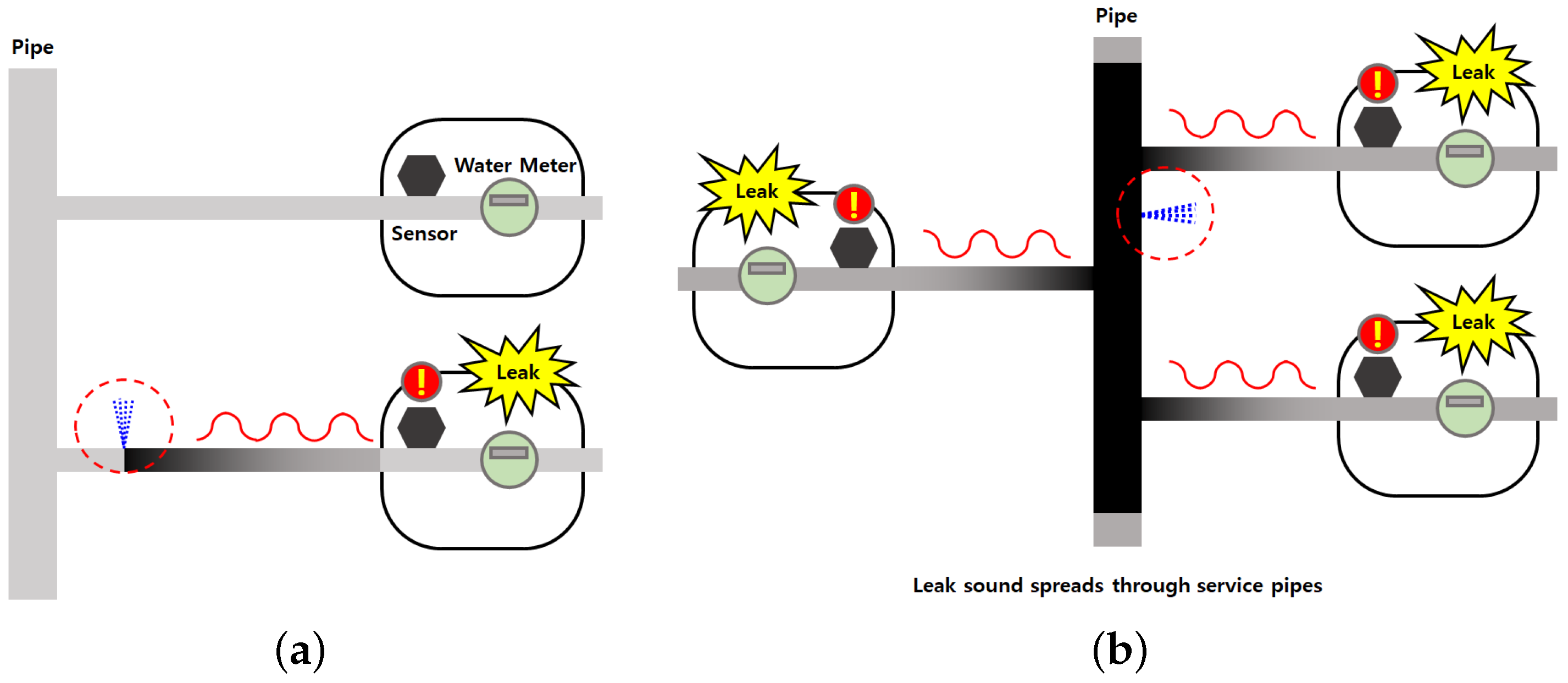
Figure 2 shows how the sensor attached to the water pipe is utilized to discriminate indoor and outdoor leakage [32]. Indoor leakage refers to the case of leakage in the water supply pipe, where leakage noise is detected by the sensor attached to the pipe, as shown in Figure 2a. In contrast, outdoor leakage refers to the case of leakage in the drain pipe. Drain pipe leakage noise is propagated to nearby water supply pipes and the sensors equipped to supply pipes around the drainpipe detect the leakage simultaneously, as shown in Figure 2b. Therefore, in this case, the leak detection signal is simultaneously transmitted from sensors near the drain.
The collected data are refined based on the decision confirmed in the field through actual leakage exploration and classified for subsequent analysis. Data types are largely divided into three types: normal, abnormal, and noise. The data are specifically labeled into five classes: outdoor leak, indoor leak, electrical/mechanical noise, environmental noise, and normal sound. The outdoor leak sound is the sound when a leak occurs in the drain pipe, and the indoor leak sound is the sound when a leak occurs in the water supply pipe. Electrical/mechanical noise is a sound mixed with electrical sound such as heating wires to prevent water pipes from freezing and bursting, and environmental sound is a sound mixed with life noise, such as the operation sound of an outdoor unit. For each class, 21,923 outdoor leaks, 16,591 indoor leaks, 6288 electrical/mechanical sounds, 8774 environmental sounds, and 24,628 typical sounds, for a total of 78,204 samples are the numbers of data samples used in the experiment were. The composition of the data is summarized in Table 1.
The sensor signals are transformed into a spectral density using 1024-FFT, with a spectral range from 0 Hz to 5120 Hz. Each datum consists of an area code, a sensor number, and spectral magnitudes according to frequency. Figure 3 shows the average magnitude spectra for the five cases. In Figure 3a, the spectra of normal sound and indoor and outdoor leak sounds can be compared, while Figure 3b shows the noise sounds, which are classified by the regular classes.

3. CNN Model

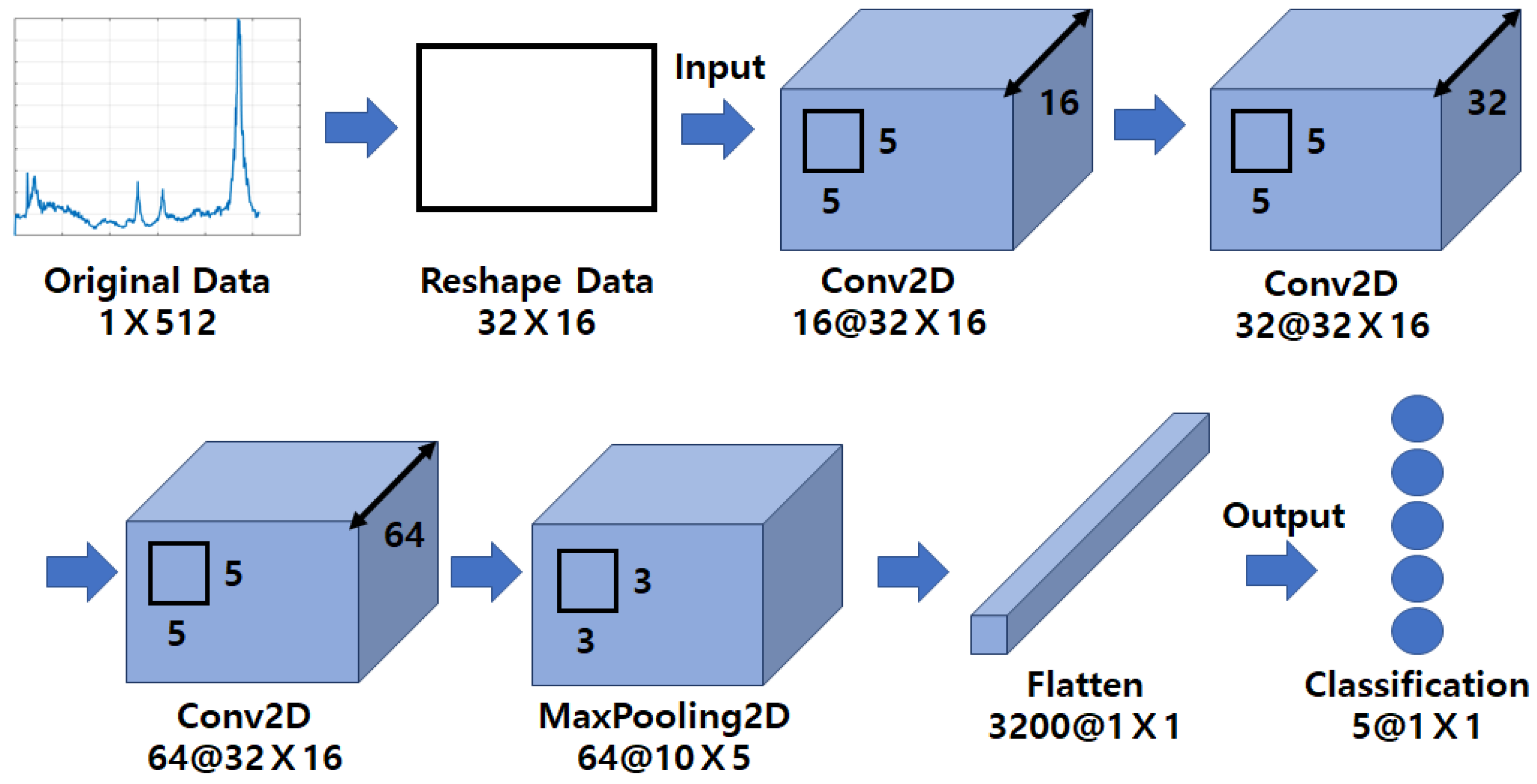
The water pipeline leak detection model is based on a 2D CNN model proposed by Lecun [33]. Figure 4 depicts the conceptual structure of the designed CNN model. In order to take advantage of the two-dimensional convolution layer, a magnitude spectrum vector of 1 × 512 is converted to a matrix of 32 × 16 as input to the CNN.
Through trial and error, the structure of the layer is changed, followed by evaluating the accuracy and loss of the model to optimize the hyperparameters. This repetition process provides gradual convergence to the range where the optimal values exist. The model with the minimum classification loss is selected as the final CNN model for water pipe leak detection.
The architecture of CNN is a multilayer feedforward neural network composed of sequentially stacked layers, as shown in Table 2, which summarizes the architecture of the proposed model with each layer type and dimension, the kernel size, and the number of connected perceptrons. There are five layers: Batch Normalization, Convolution, Maxpooling, Flatten, and Fully Connected Layers. Since the features have a density of 512 frequency components, the CNN input layer takes an input matrix of 32 × 16 for better training. The first layer performs batch normalization, which normalizes the input data. The number of filters is set to 16 in the second layer, i.e., the convolution layer. Here, the kernel size is 5 × 5 , and the rectified linear unit activation function is used. This structure is repeated twice by increasing the number of two-dimensional convolution filters to 32 and 64. Between the consecutive convolution layers, a batch normalization layer is added to prevent the slope loss problem and congestion. After configuring up to the sixth layer, max pooling is performed at the seventh layer. The max pooling layer has a kernel size of 3 × 3 . The eighth layer is a Flatten lay, and all nodes are fully connected. The flattening layer converts two-dimensional information into one dimension and transfers the characteristics acquired from the convolution and the pooling layers to the fully connected layer. In the ninth layer, i.e., the fully connected layer, 3200 nodes are fully connected to five nodes, and the data are classified into five classes through the softmax function. The total number of nodes used in this model was 80,713. We used a cross-entropy loss function and the Adam optimizer.

4. SVM Model

For the purpose of comparison, as mentioned previously, the SVM model is employed. The radial basis function (RBF) is adopted for the SVM model [34], which is defined as
K R B F ( x 1 , x 2 ) = e x p ( x 1 x 2 2 2 σ 2 ) ,
where x 1 and x 2 are the data points, · implies the Euclidean distance, and 2 σ 2 is a parameter that controls the width of the RBF kernel. This is set to the dimension of the feature vector X as follows:
2 σ 2 = D i m ( X ) ,
Since SVM models can use vectors as input features, the input feature of the SVM model is a vector of 1 × 512 , which is the same as that of the CNN model without shape conversion. The feature vector undergoes a scaling process using a standard scaler to prevent the cost value from diverging and not being trained normally.
In the experiment, the value for the cost function is set to 10, and the value of the kernel is set to 512, which is the dimension of the feature vector X.

5. Experiment

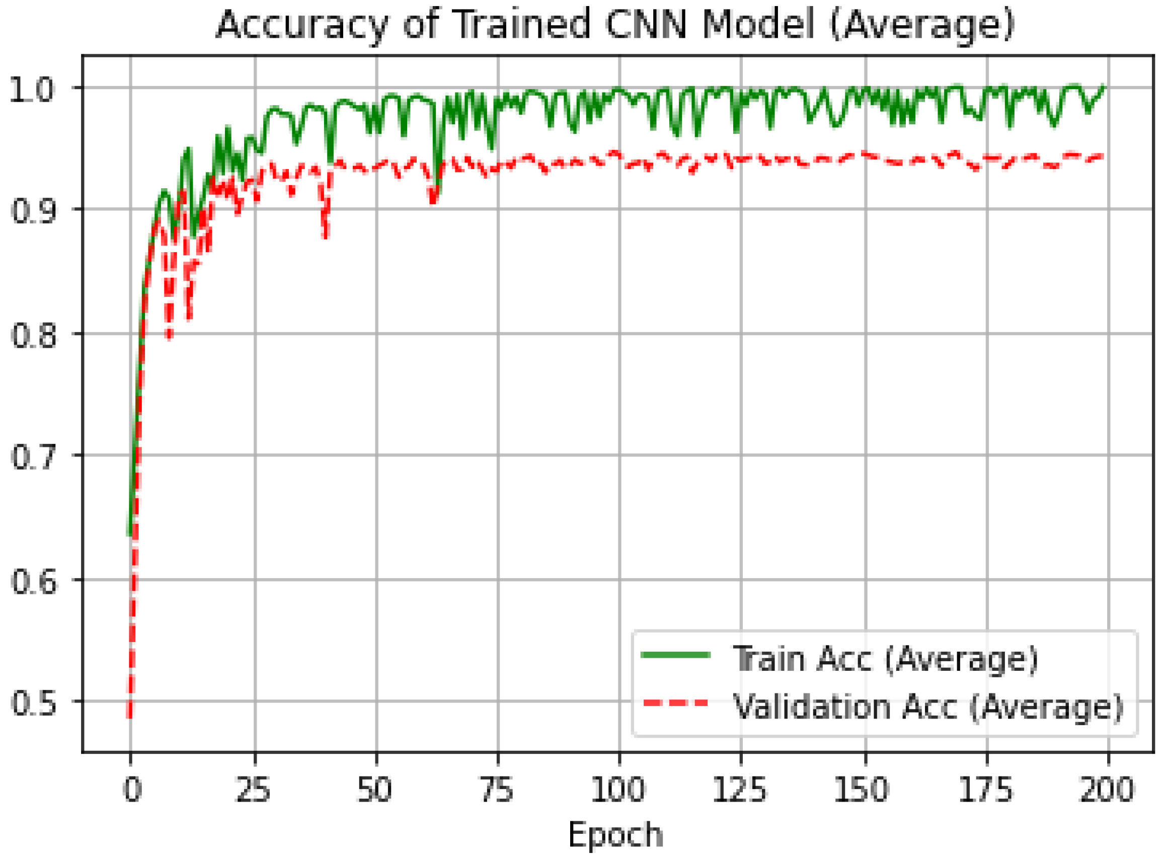
Each dataset utilized in this experiment consists of a total of 78,204 data; 50,050 training data, 12,513 validation data, and 15,641 test data. The investigation was carried out 50 times over the randomly selected data sets, the construction ratio of which was maintained. The results presented in this section are based on the average of the 50 runs. The CNN model updates the weights whenever the verification loss is reduced in the learning process. The early termination condition for the training process was set to proceed with 100 additional epochs of training from the point of update. Although all models satisfied the early termination condition in less than 200 epochs, we continued training up to epochs for visual comparison.
Figure 5 shows a graph of the training and validation accuracy over different training epochs. These values were obtained by averaging the 50 models as mentioned previously. The training and validation loss is shown in Figure 6.
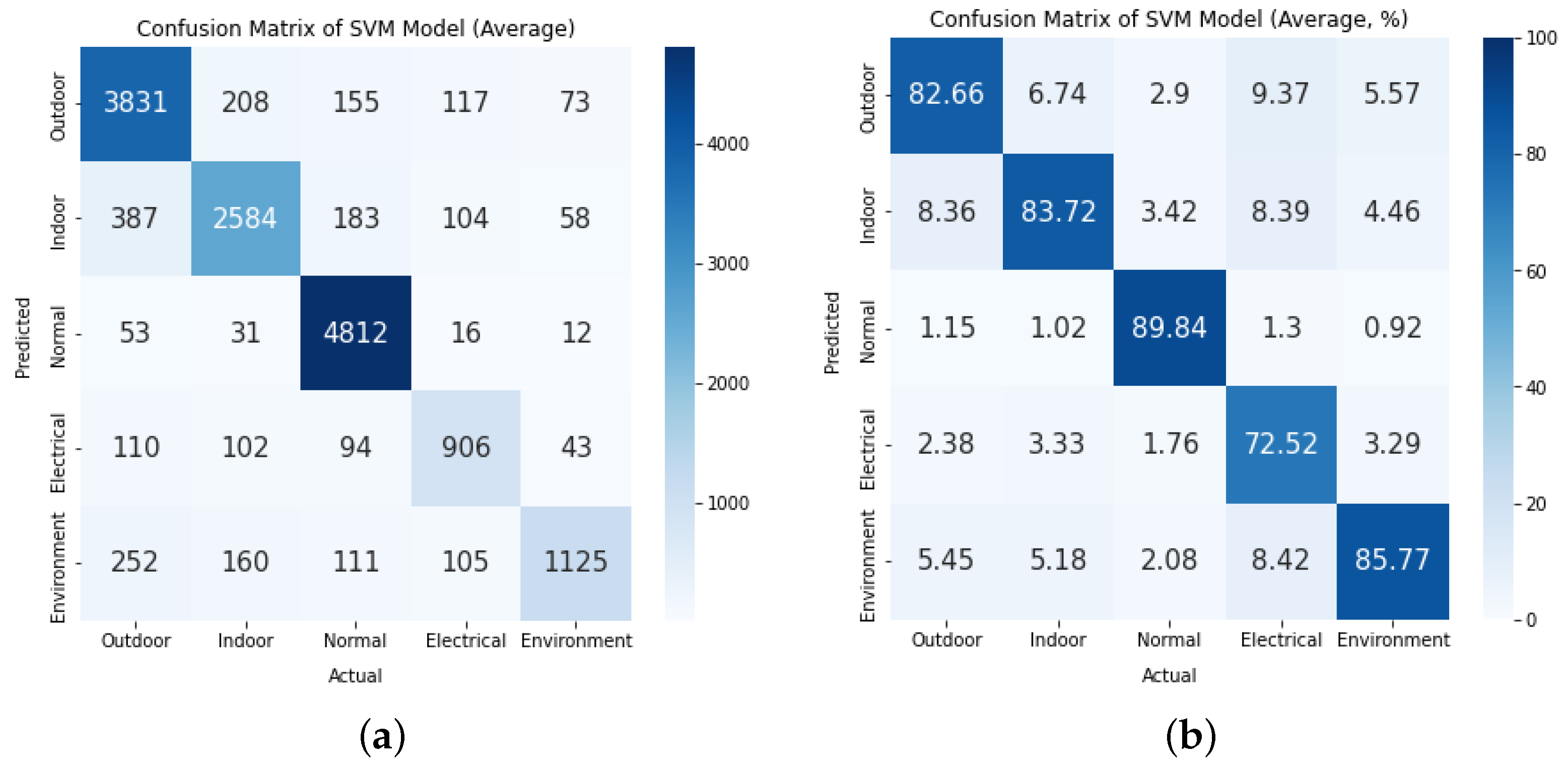
The performance of each CNN model was investigated by classifying 15,641 test data into five classes. The average confusion matrix over the 50 CNN models is presented in Figure 7. In addition, that of the SVM models can be found in Figure 8. Comparing both matrices reveal that the diagonal components of the CNN model were greater than those of the SVM model, which implies that the CNN models performed better. Five performance metrics, including precision, recall, accuracy, F1 score, and Matthew’s correlation coefficient (MCC), were employed to obtain clear insight into the performance comparison. The precision, recall, and accuracy are, respectively, defined as follows [35,36].
Precision = T P T P + F P ,
Recall = T P T P + F N ,
and
Accuracy = T P + T N T P + T N + F P + F N ,
where T P , T N , F P , and F N stand for true positive, true negative, false positive, and false negative, respectively.
As may be observed from Equations (3) and (4), precision and recall indicators evaluate the true predictions. In addition, because predicting false data as false is correct, the accuracy metric evaluates both TP and TN. The data used in this study had an imbalanced ratio by class. In the case of model performance evaluation, simply using accuracy as an evaluation metric can lead to a significant accuracy bias when the data are imbalanced. For this reason, the F1 score and MCC, which can complement this, are employed as additional metrics. The F1 score is the harmonic average of the precision and recall, which is defined as
F 1 score = 2 × Precision × Recall Precision + Recall = T P T P + 1 2 ( F P + F N )
This can accurately evaluate the performance of an unbiased model even when the data ratio for each class is imbalanced [37].
As another measure that compensates for the unbalanced datasets issue, MCC measures the correlation between an actual class and a prediction class. MCC for G classes is defined as in [36,38]
MCC = c × s g G p g × t g ( s 2 g G p g 2 ) ( s 2 g G t g 2 ) ,
where the total number of correctly predicted elements is denoted by c = g G C g g , the total number of elements s = i G j G C i j , the number of times that class g was predicted (column total) p g = i G C g i , and the number of times that class g truly occurred (row total) t g = i G C i g . It ranges in [ 1 , + 1 ] , where the value 1 represents the case of perfect misclassification, the value + 1 does the case of perfect classification, and M C C = 0 does the coin tossing classifier.
MCC can also be used to evaluate the performance of a model with an unbalanced ratio of data between classes, such as F1-score [39,40]. The F1 score depends on which class is defined as positive in Equation (6). However, MCC is an indicator that has the advantage of preventing a positive class from being incorrectly defined over an F1 score because it does not depend on which class is positive.
Table 3 summarizes the performance of the CNN and SVM models in terms of precision, recall, accuracy, F1 score, and MCC, respectively. In each evaluation, precision, recall, and F1 score were calculated for each class, and then the macro-averaged values were reported as each model’s final values. The values shown in Table 3 are obtained by averaging over 50 runs.
According to Table 3, the trained CNN model exhibited better recall performance than precision, whereas the SVM model showed better precision performance than recall. This means that when the trained CNN model classifies a data sample, it is essential not to classify it incorrectly. Conversely, SVM models focus on classifying data into actual categories. The CNN model performed better than the SVM model in terms of accuracy. As mentioned, accuracy may be biased due to an imbalanced dataset issue. Precision and recall have relatively little meaning when viewed alone due to differences in perspective; hence, the performance was evaluated using the F1 score and MCC. These indices comprehensively look at precision and recall at once.
The difference between the accuracy and the F1 score in the CNN model is about 1%, whereas the difference in the SVM model is 3.8%. This means that compared to the SVM model, the bias in classifying the CNN model is less. Furthermore, the MCC of the CNN model is 0.9447, and that of the SVM model is 0.7986, indicating that the CNN model can be classified similarly to the actual correct answer compared to the SVM model. As a result of using various indicators to evaluate the model, the CNN model shows excellent classification performance without being biased to a specific class in leak detection classification prediction.

6. Conclusions

Because experts are required to visit the site to detect leaks through the existing hearing leak exploration technique, there have been considerable research and development for remote leak detection, such as using IoT-based water pipeline monitoring systems. In this study, we proposed application of a CNN model to detect leaks in a water pipeline by automating leak exploration techniques that rely on the personal capabilities of experts. Using the leak sensor data, the leak detector learns the leak data, which are divided into five classes, and finally determines whether a leak has occurred. We selected a CNN model; 62,563 data samples were collected as a training dataset, and the performance was evaluated with 15,641 samples. For a reliable investigation, 50 models were developed and tested. The results presented in the paper are based on the average performance of the 50 CNN models. Five performance metrics were used for evaluation, including precision, recall, accuracy, F1 score, and MCC. For comparison, an SVM model was also applied under the same environment. The performance of the CNN model was superior to that of the SVM.
The CNN-based water pipe leak detection model proposed in this work can help develop an intelligent leak detection system. This study demonstrates the validity of artificial intelligence-based automatic leak detection. Note in this study that the data are supposed to be collected in a data hub and that the proposed model is implemented in a higher-level language. Thus, the sound samples should be periodically transmitted through wireless networks from sensor nodes, especially long-term evolution networks in this study. This results in high transmission traffic, which is not desirable.
To overcome this disadvantage, the data traffic amount should be lowered. One way is employing a detection model that can be installed in the sensor module. The module only sends an alarm to the management center when the detection model detects an abnormal condition. For this development, the complexity of the model should be so low that it can be implemented in low-level hardware without loss of performance. This development is challenging, and the application of other machine learning models will be investigated for this development. More essential features that can reflect leakage more effectively should be studied in the time and frequency domain.

Author Contributions

J.C. and S.I. contributed to writing, reviewing, and editing the paper. All authors have read and agreed to the published version of the manuscript.

Funding

This work was supported by the National Research Foundation of Korea (NRF) grant funded by the Korea government (MSIT) (No. NRF-2021R1F1A1061403).

Institutional Review Board Statement

Not applicable.

Informed Consent Statement

Not applicable.

Data Availability Statement

Restrictions apply to the availability of these data. Data were obtained from AI Hub, and are available from the authors with the permission of AI Hub.

Acknowledgments

The authors would like to express thanks to AI Hub for providing the experiment datasets.

Conflicts of Interest

The authors declare no conflict of interest.

References

  1. Choi, Y.H.; Kim, Y.R. Research Regard to Necessity of Smart Water Management Based on IoT Technology. J. Korea Ind. Inf. Syst. Res. 2017, 22, 11–18. [Google Scholar]
  2. Yoon, D.J.; Jeong, J.C.; Lee, Y.S. Leak detection of waterworks pipeline using acoustic emission and correlation method. In Proceedings of the KSME Conference, Busan, Korea, 23–25 April 2003; pp. 84–89. [Google Scholar]
  3. Colombo, A.F.; Karney, B.W. Energy and costs of leaky pipes: Toward comprehensive picture. J. Water Resour. Plan. Manag. 2002, 128, 441–450. [Google Scholar] [CrossRef] [Green Version]
  4. Xin, K.; Li, F.; Tao, T.; Xiang, N.; Yin, Z. Water losses investigation and evaluation in water distribution system—The case of SA city in China. Urban Water J. 2015, 12, 430–439. [Google Scholar] [CrossRef]
  5. Fuentes, H.; Mauricio, D. Smart water consumption measurement system for houses using IoT and cloud computing. Environ. Monit. Assess. 2020, 192, 1–16. [Google Scholar]
  6. Jan, F.; Min-Allah, N.; Saeed, S.; Iqbal, S.Z.; Ahmed, R. IoT-Based Solutions to Monitor Water Level, Leakage, and Motor Control for Smart Water Tanks. Water 2022, 14, 309. [Google Scholar]
  7. Rabeek, S.M.; Beibei, H.; Chai, K.T. Design of Wireless IoT Sensor Node & Platform for Water Pipeline Leak Detection. In Proceedings of the 2019 IEEE Asia-Pacific Microwave Conference (APMC), Singapore, 10–13 December 2019; IEEE: New York, NY, USA, 2019; pp. 1328–1330. [Google Scholar]
  8. Choi, S.H.; Eom, D.S. Wireless Water Leak Detection System Using Sensor Networks. J. Inst. Electron. Eng. Korea 2011, 48, 125–131. [Google Scholar]
  9. Choi, J.; Shin, J.; Song, C.; Han, S.; Park, D.I. Leak detection and location of water pipes using vibration sensors and modified ML prefilter. Sensors 2017, 17, 2104. [Google Scholar] [CrossRef] [Green Version]
  10. Chuang, W.Y.; Tsai, Y.L.; Wang, L.H. Leak detection in water distribution pipes based on CNN with mel frequency cepstral coefficients. In Proceedings of the 2019 3rd International Conference on Innovation in Artificial Intelligence, Suzhou, China, 15–18 March 2019; pp. 83–86. [Google Scholar]
  11. Choi, Y.; Cho, W. Research of Automatic Water Leak Detection Technology Used on Thermography and Deep Learning. J. Korean Inst. Inf. Technol. 2018, 16, 1–9. [Google Scholar]
  12. Ravichandran, T.; Gavahi, K.; Ponnambalam, K.; Burtea, V.; Mousavi, S.J. Ensemble-based machine learning approach for improved leak detection in water mains. J. Hydroinform. 2021, 23, 307–323. [Google Scholar] [CrossRef]
  13. Zhou, B.; Lau, V.; Wang, X. Machine-learning-based leakage-event identification for smart water supply systems. IEEE Internet Things J. 2019, 7, 2277–2292. [Google Scholar]
  14. Li, J.; Liu, Y.; Chai, Y.; He, H.; Gao, M. A Small Leakage Detection Approach for Gas Pipelines based on CNN. In Proceedings of the 2019 CAA Symposium on Fault Detection, Supervision and Safety for Technical Processes (SAFEPROCESS), Xiamen, China, 5–7 July 2019; IEEE: New York, NY, USA, 2019; pp. 390–394. [Google Scholar]
  15. Ning, F.; Cheng, Z.; Meng, D.; Duan, S.; Wei, J. Enhanced spectrum convolutional neural architecture: An intelligent leak detection method for gas pipeline. Process Saf. Environ. Prot. 2021, 146, 726–735. [Google Scholar]
  16. Ismail, M.I.M.; Dziyauddin, R.A.; Salleh, N.A.A.; Muhammad-Sukki, F.; Bani, N.A.; Izhar, M.A.M.; Latiff, L.A. A review of vibration detection methods using accelerometer sensors for water pipeline leakage. IEEE Access 2019, 7, 51965–51981. [Google Scholar] [CrossRef]
  17. Waleed, D.; Mustafa, S.H.; Mukhopadhyay, S.; Abdel-Hafez, M.F.; Jaradat, M.A.K.; Dias, K.R.; Arif, F.; Ahmed, J.I. An in-pipe leak detection robot with a neural-network-based leak verification system. IEEE Sens. J. 2018, 19, 1153–1165. [Google Scholar] [CrossRef]
  18. Ong, K.; Png, W.; Lin, H.; Pua, C.; Rahman, F. Acoustic vibration sensor based on macro-bend coated fiber for pipeline leakage detection. In Proceedings of the 2017 17th International Conference on Control, Automation and Systems (ICCAS), Jeju, Korea, 18–21 October 2017; IEEE: New York, NY, USA, 2017; pp. 167–171. [Google Scholar]
  19. Spandonidis, C.; Theodoropoulos, P.; Giannopoulos, F.; Galiatsatos, N.; Petsa, A. Evaluation of deep learning approaches for oil & gas pipeline leak detection using wireless sensor networks. Eng. Appl. Artif. Intell. 2022, 113, 104890. [Google Scholar]
  20. Spandonidis, C.; Theodoropoulos, P.; Giannopoulos, F. A Combined Semi-Supervised Deep Learning Method for Oil Leak Detection in Pipelines Using IIoT at the Edge. Sensors 2022, 22, 4105. [Google Scholar]
  21. Li, Q.; Shi, Y.; Lin, R.; Qiao, W.; Ba, W. A novel oil pipeline leakage detection method based on the sparrow search algorithm and CNN. Measurement 2022, 204, 112122. [Google Scholar]
  22. Yu, Y.; Samali, B.; Rashidi, M.; Mohammadi, M.; Nguyen, T.N.; Zhang, G. Vision-based concrete crack detection using a hybrid framework considering noise effect. J. Build. Eng. 2022, 61, 105246. [Google Scholar]
  23. Yu, Y.; Liang, S.; Samali, B.; Nguyen, T.N.; Zhai, C.; Li, J.; Xie, X. Torsional capacity evaluation of RC beams using an improved bird swarm algorithm optimised 2D convolutional neural network. Eng. Struct. 2022, 273, 115066. [Google Scholar]
  24. Zha, W.; Liu, Y.; Wan, Y.; Luo, R.; Li, D.; Yang, S.; Xu, Y. Forecasting monthly gas field production based on the CNN-LSTM model. Energy 2022, 260, 124889. [Google Scholar]
  25. Meniconi, S.; Capponi, C.; Frisinghelli, M.; Brunone, B. Leak detection in a real transmission main through transient tests: Deeds and misdeeds. Water Resour. Res. 2021, 57, e2020WR027838. [Google Scholar]
  26. Brunone, B.; Maietta, F.; Capponi, C.; Keramat, A.; Meniconi, S. A review of physical experiments for leak detection in water pipes through transient tests for addressing future research. J. Hydraul. Res. 2022, 60, 894–906. [Google Scholar] [CrossRef]
  27. Vapnik, V. An overview of statistical learning theory. IEEE Trans. Neural Netw. 1999, 10, 988–999. [Google Scholar] [CrossRef] [Green Version]
  28. Platt, J. Sequential Minimal Optimization: A Fast Algorithm for Training Support Vector Machines; Technical Report MSR-TR-98-14; Microsoft: Washington, DC, USA, 1998. [Google Scholar]
  29. Mandal, S.K.; Chan, F.T.; Tiwari, M. Leak detection of pipeline: An integrated approach of rough set theory and artificial bee colony trained SVM. Expert Syst. Appl. 2012, 39, 3071–3080. [Google Scholar] [CrossRef]
  30. Sun, J.; Xiao, Q.; Wen, J.; Wang, F. Natural gas pipeline small leakage feature extraction and recognition based on LMD envelope spectrum entropy and SVM. Measurement 2014, 55, 434–443. [Google Scholar] [CrossRef]
  31. Gao, Y.; Brennan, M.; Joseph, P.; Muggleton, J.; Hunaidi, O. On the selection of acoustic/vibration sensors for leak detection in plastic water pipes. J. Sound Vib. 2005, 283, 927–941. [Google Scholar] [CrossRef]
  32. AI-Hub, Water and Sewage Data (Water Pipeline Leak Detection). Available online: https://www.aihub.or.kr/aihubdata/data/view.do?currMenu=115&topMenu=100&aihubDataSe=realm&dataSetSn=138 (accessed on 23 December 2022).
  33. LeCun, Y.; Bottou, L.; Bengio, Y.; Haffner, P. Gradient-based learning applied to document recognition. Proc. IEEE 1998, 86, 2278–2324. [Google Scholar] [CrossRef] [Green Version]
  34. Han, S.; Qubo, C.; Meng, H. Parameter selection in SVM with RBF kernel function. In Proceedings of the World Automation Congress 2012, Puerto Vallarta, Mexico, 24–28 June 2012; IEEE: New York, NY, USA, 2012; pp. 1–4. [Google Scholar]
  35. Powers, D.M. Evaluation: From precision, recall and F-measure to ROC, informedness, markedness and correlation. arXiv 2020, arXiv:2010.16061. [Google Scholar]
  36. Grandini, M.; Bagli, E.; Visani, G. Metrics for Multi-Class Classification: An Overview. arXiv 2020, arXiv:2008.05756. [Google Scholar] [CrossRef]
  37. Jeni, L.A.; Cohn, J.F.; De La Torre, F. Facing imbalanced data–recommendations for the use of performance metrics. In Proceedings of the 2013 Humaine Association Conference on Affective Computing and Intelligent Interaction, Geneva, Switzerland, 2–5 September 2013; IEEE: New York, NY, USA, 2013; pp. 245–251. [Google Scholar]
  38. Gorodkin, J. Comparing two K-category assignments by a K-category correlation coefficient. Comput. Biol. Chem. 2004, 28, 367–374. [Google Scholar] [CrossRef]
  39. Chicco, D.; Jurman, G. The advantages of the Matthews correlation coefficient (MCC) over F1 score and accuracy in binary classification evaluation. BMC Genom. 2020, 21, 1–13. [Google Scholar] [CrossRef] [Green Version]
  40. Chicco, D.; Tötsch, N.; Jurman, G. The Matthews correlation coefficient (MCC) is more reliable than balanced accuracy, bookmaker informedness, and markedness in two-class confusion matrix evaluation. BioData Min. 2021, 14, 1–22. [Google Scholar] [CrossRef] [PubMed]
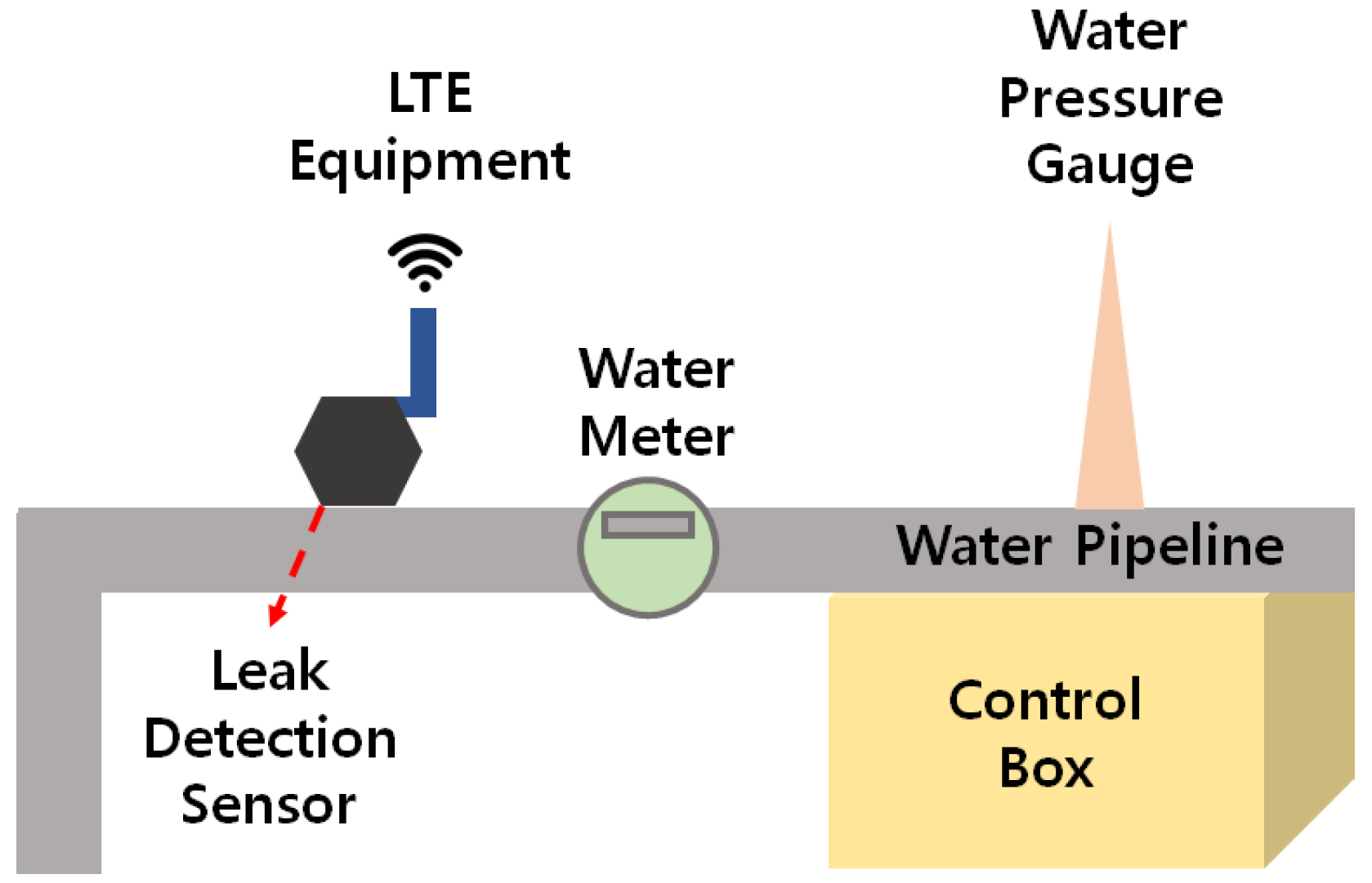
Figure 1. A flow and water pressure monitoring module was used to collect data [32].
Applsci 13 02845 g001
Figure 2. Detection scenarios. (a) Indoor water leak and (b) outdoor water leak.
Applsci 13 02845 g002
Figure 3. Average magnitude spectra of five classes. (a) Normal Sound vs. Leak Sounds and (b) Normal Sound vs. Noise Sounds.
Applsci 13 02845 g003
Figure 4. Structure of the CNN model used in the water pipeline leak detection.
Applsci 13 02845 g004
Figure 5. Average training accuracy and validation accuracy of the 50 CNN models.
Applsci 13 02845 g005
Figure 6. Average training loss and validation loss of the 50 CNN models.
Applsci 13 02845 g006
Figure 7. Average confusion matrix of the 50 CNN models. (a) In number and (b) in percentage.
Applsci 13 02845 g007
Figure 8. Average confusion matrix of the 50 SVM models. (a) In number and (b) in percentage.
Applsci 13 02845 g008
Table 1. Data composition summary.
TypeLabelNumber
NormalNormal24,628
AnomalyOutdoor Leakage21,923
Indoor Leakage16,591
NoiseElectrical/Mechanical6288
Environmental8774
Total 78,204
Table 2. Summary of the trained CNN model.
LayerTypeDimensionKernel SizeParameter #
1Batch Normalization1@32 × 16 5 × 5 4
2Convolution16@32 × 16 5 × 5 416
3Batch Normalization16@32 × 165 × 564
4Convolution32@32 × 165 × 512,832
5Batch Normalization32@32 × 165 × 5128
6Convolution64@32 × 165 × 551,264
7Maxpooling64@10 × 53 × 3-
8Flatten3200@1 × 1--
9Fully Connected5@1 × 1-16,005
10Output5@1 × 1--
Table 3. Performance summary of the CNN and SVM models, obtained by averaging over 50 runs.
Evaluation MetricCNNSVM
Precision0.94710.8295
Recall0.94970.7984
Accuracy0.95800.8478
F1 score0.94820.8099
MCC0.94470.7986
Disclaimer/Publisher’s Note: The statements, opinions and data contained in all publications are solely those of the individual author(s) and contributor(s) and not of MDPI and/or the editor(s). MDPI and/or the editor(s) disclaim responsibility for any injury to people or property resulting from any ideas, methods, instructions or products referred to in the content.