Abstract
This paper presents a proposal of an efficient binaural room-acoustics auralization method, an essential goal of room-acoustics modeling. The method uses a massively parallel wave-based room-acoustics solver based on a dispersion-optimized explicit time-domain finite element method (TD-FEM). The binaural room-acoustics auralization uses a hybrid technique of first-order Ambisonics (FOA) and head-related transfer functions. Ambisonics encoding uses room impulse responses computed by a parallel wave-based room-acoustics solver that can model sound absorbers with complex-valued surface impedance. Details are given of the novel procedure for computing expansion coefficients of spherical harmonics composing the FOA signal. This report is the first presenting a parallel wave-based solver able to simulate room impulse responses with practical computational times using an HPC cloud environment. A meeting room problem and a classroom problem are used, respectively, having 35 million degrees of freedom (DOF) and 100 million DOF, to test the parallel performance of up to 6144 CPU cores. Then, the potential of the proposed binaural room-acoustics auralization method is demonstrated via an auditorium acoustics simulation of up to 5 kHz having 750,000,000 DOFs. Room-acoustics auralization is performed with two acoustics treatment scenarios and room-acoustics evaluations that use an FOA signal, binaural room impulse response, and four room acoustical parameters. The auditorium acoustics simulation showed that the proposed method enables binaural room-acoustics auralization within 13,000 s using 6144 cores.
1. Introduction
Room-acoustics control with acoustical materials such as sound absorbers and acoustic diffusers is necessary for creating an acoustically comfortable indoor sound environment that positively affects people’s performance and health. Room-acoustics simulation methods are crucially important for the acoustic design of architecture spaces, providing room impulse responses (RIRs) for room-acoustics evaluations. One can calculate various room-acoustics parameters such as reverberation times from RIRs. The RIRs are also available for room-acoustics visualization and auralization [1]. Wave-based acoustic simulations [2] are intrinsically more favored as acoustics design tools compared to geometrical acoustic simulations [3] because they can accurately describe acoustical effects associated with room shapes and acoustic materials. Nevertheless, wave-based acoustics simulations are well known to have an important shortcoming: high computational costs for practical applications. Auralization of room acoustics at wide bands is exceedingly difficult. Despite this inefficiency, development of computationally efficient parallel acoustic simulation methods has been explored [4,5,6,7,8,9]. Consequently, the applicable range of wave-based acoustics simulations is expanding radically: wave-based room-acoustics auralization is becoming a practical alternative. This report describes a specific examination of a recently developed highly parallel wave-based room-acoustics solver: the dispersion-optimized explicit time-domain finite element method (TD-FEM) [9]. The findings underscore its potential for binaural auralization of room acoustics.
Dispersion-optimized explicit TD-FEM [9,10] is a domain decomposition method (DDM) based acoustics simulation solver that uses a dispersion-optimized low-order finite element (FE) and a specially designed time integration method. It can model acoustic materials by frequency-dependent local-reaction complex-valued impedance boundary conditions. The explicit TD-FEM has higher efficiency and accuracy than standard TD-FEM with low-order FEs. It enables the use of lower-resolution meshes than the standard TD-FEM to compute more accurate RIRs. As an appealing feature, the explicit TD-FEM code can be generated from the standard FEM codes with linear hexahedral elements. Preliminary work [9] demonstrated the basic practicality of the explicit TD-FEM via room-acoustics simulation in a large-scale auditorium of up to 3 kHz under a parallel computing system with 512 cores. In fact, DDM-based solvers can accommodate massively parallel computing environments such as cloud high-performance computing (HPC) systems. Therefore, DDM-based explicit FEM can be an attractive technology for realizing wave-based auralization of room acoustics. However, its potential for room-acoustics auralization remains unclear.
In room-acoustics auralization, appropriately perceiving spatial auditory scenes in simulated sound fields requires the computation of binaural RIRs (BRIRs). The most straightforward approach to computing BRIRs in the listener’s two ears is to include a human head model with pinnae into a 3D room model in room-acoustics simulation. However, this approach requires high computational costs because it requires modeling of an extremely complex human head geometry. Moreover, one can only compute BRIRs for a single head orientation. Multiple simulations are necessary to consider a listener’s head movement. Hybrid approaches combining sound field reproduction methods such as wave field synthesis [11], boundary surface control [12] and Ambisonics [13,14], and head-related transfer functions (HRTF) have been proposed. Hybrid approaches are attractive for binaural auralization because they can produce binaural signals in arbitrary head orientation without modeling the human head in room-acoustics simulation. Among the others, hybrid auralization with Ambisonics and HRTF [15,16] has high compatibility with virtual reality (VR) applications [17,18].
In Ambisonics, the sound field is expressed by the superposition of plane waves based on spherical harmonics expansion. The Ambisonics signal consists of expansion coefficients of spherical harmonics up to the desired order in the time domain at an arbitrary point in an interested sound field. Standard Ambisonics auralization is performed by assigning Ambisonics signals to an arbitrary speaker array so that the original sound field is reproduced at the center of the speaker array. For combination with HRTF, driving signals are assigned to the virtual speaker array instead of the real speaker array. Then, binaural signals are synthesized via convolution of each driving signal with head-related impulse response (HRIR) in the same direction of each virtual speaker. Ambisonics are roughly classified into first-order Ambisonics (FOA) [13] consisting of the zero-order and first-order expansion coefficients and higher-order Ambisonics (HOA) [14], with coefficients of up to the second order and higher. Although HOA sound reproduction can capture a sound field well compared to FOA reproduction, FOA is often applied to architectural acoustics problems such as acoustics evaluation of churches [19], concert halls [20], underground railway stations [21], and meeting rooms [22]. Some plugins for FOA to VR applications are available.
This paper presents a proposal of a binaural room-acoustics auralization method based on FOA reproduction using a massively parallel wave-based room-acoustics solver by dispersion-optimized explicit TD-FEM, with examination of the efficiency and feasibility of the method. The proposed method first computes RIRs by the parallel wave-based solver under a cloud HPC environment. Then, BRIRs are computed using a hybrid approach with FOA and HRTF. Room acoustics auralization is presented to a listener via headphones. For the BRIR rendering, a novel computational method to compute expansion coefficients of spherical harmonics via numerical differentiation using finite element’s shape function is proposed. First, this study assesses the efficiency of the massively parallel wave-based room-acoustics solver via a scalability test on a cloud HPC environment with two realistic room-acoustics simulations in a meeting room and classroom. Then, the potential of the proposed binaural room-acoustics auralization method is shown via acoustics simulations in a large auditorium of up to 5 kHz.
2. Theory
This section presents a theory of the proposed binaural room-acoustics auralization method using a massively parallel wave-based room-acoustics solver. First, the relevant theory of the massively parallel wave-based room-acoustics solver is given briefly: dispersion-optimized explicit TD-FEM with DDM-based parallel computing implementation. Spatial discretization is consistently performed with eight-node linear hexahedral FEs in the study. Then, the theory of a hybrid binaural room-acoustics auralization method based on Ambisonics with HRTF is given. A novel approach is also formulated for accessing expansion coefficients of spherical harmonics using spatial differentiation of the finite element shape function.
2.1. Massively Parallel Room Acoustics Solver
2.1.1. Dispersion-Optimized Explicit TD-FEM
Room-acoustics simulation in a time domain solves the following second-order scalar wave equation related to sound pressure p as
with the following three boundary conditions (BCs): The rigid BC , the vibration BC , and the impedance BC .
Here, q and respectively denote the volume velocity per unit volume and the vibration velocity in a normal direction on the boundary surface. and respectively express the Laplacian operator and the Dirac delta function. In addition, and respectively represent the speed of sound and the air density. In addition, and respectively stand for the arbitrary coordinate vector in a computational domain and the coordinate vector of a point source. Symbol · is the first-order time derivative of . stands for the specific acoustic admittance ratio of materials in the time domain. Impedance BC involves the convolution to address the frequency dependency of . Applying Galerkin FE approximation into Equation (1) yields semi-discretized FE equation as
Therein, , , and respectively represent the global consistent mass matrix, the global stiffness matrix, and the global dissipation matrix composed with each element matrix , , and . and respectively represent the vectors for sound pressure and external forces. Symbols and * respectively symbolize the second-order time derivative and convolution operator. Dispersion-reduced TD-FEM [23,24] solves Equation (3) directly to compute RIRs, but the resulting time-marching scheme shows an implicit algorithm, which requires the solution of a linear system of equations at each time step.
The dispersion-optimized explicit TD-FEM [9,10] solves the following simultaneous first-order ODEs, which is equivalent to Equation (3), with approximation of convolution relevant to the impedance BC by the auxiliary differential equations (ADE) method [25]:
In the equations mentioned above, represents the lumped mass matrix converted from using the row-sum method [26]. Additionally, denotes the auxiliary vector equivalent to the first derivative of with respect to time. The ADE method efficiently computes the convolution integral using an approximated acoustic admittance function form at angular frequency in the frequency domain. The function form is expressed with the real poles , the pairs of complex conjugate poles with the imaginary unit , and real-valued parameters , , and as follows:
Therein, and are the numbers of real poles and complex conjugate pole pairs. It is crucially important that the approximated admittance with multi-pole model be causal and passive for reasons of stability. The dispersion-optimized explicit TD-FEM minimizes the dispersion error at a specific frequency for sound waves propagating in the axial and diagonal directions of the Cartesian system with special integration points for calculating and . The time-marching scheme is formulated using a dissipation-free three-step time integration method [10] to Equation (4), the first-order backward difference to and the first-order central difference to in Equation (5), and the Crank–Nicolson method to Equations (6)–(8). The complete expression of the time-marching scheme is given as
with
Therein, denotes the time interval; in addition, n stands for the time step. is the optimization parameter for minimizing temporal dispersion error at a specific frequency. In later numerical experiments, dispersion error optimizations are conducted following earlier reports of the relevant literature [9,10]. All equations are explicit in the time-marching scheme presented above, except for Equation (11). Equation (11) must solve implicitly for stability reasons [27]. Fortunately, Equation (11) can be solved efficiently because we only solve the equation for impedance BC’s related nodes. Therefore, most of the systems are solvable explicitly as
An iterative solver, the conjugate residual method with a convergence tolerance of 10, is an effective means of solving Equation (11).
2.1.2. DDM-Based Parallel Computation
The DDM-based parallel computing strategy implemented into the explicit TD-FEM is described here. Actually, DDM-based parallel computing techniques of two kinds can use overlapping or non-overlapping subdomains. The present explicit TD-FEM uses non-overlapping subdomains. The DDM-based parallel computation performs each subdomain calculation simultaneously by distributing subdomains into different computational nodes or processors while communicating with other computation processes. The message passing interface (MPI) is used for communication.
In our implementation, the whole FE volume mesh is first partitioned into the non-overlapping subdomain FEs as a pre-process of room-acoustics simulations. The Metis Library [28] was used for partitioning. Then, in the room-acoustics simulation phase, each computational process reads the assigned subdomain FE volume mesh file. It enables us to compute the matrices , , and rapidly. All processes read the same global surface mesh file for constructing boundary condition matrix for ease of implementation. This boundary condition management increases the computational time of matrix construction in massively parallel computation cases because it induces competition in the file reading among the computational processes. Nevertheless, its effect on the total computational time is quite small because the matrix composition wastes much less time than the time-marching computation time, as explained in Section 3. After finishing matrix constructions, each process conducts time-marching calculations in parallel. Details of the procedure were presented in our earlier work [9].
2.2. Binaural Auralization Based on Ambisonics and HRTF
Ambisonics is a sound field reproduction method based on the spherical harmonics expansion of sound fields in which frequency-domain sound pressure is expressed as [29]
In that equation, k and r respectively stand for the wave number and radius in a polar coordinate system. In addition, represents the l-th order spherical Bessel function. The expansion coefficient for spherical harmonics is represented by . is the real spherical harmonics, denoted as
with
and represents the associated Legendre function. In addition, and respectively signify the elevation and azimuth in the spherical coordinate system. Equation (20) can be rewritten with an equation of plane wave in Cartesian coordinates as
with
The latter expression is useful to evaluate in the Cartesian coordinate system, as explained in Section 2.2. For sound field reproduction by Ambisonics, time-domain expansion coefficients up to a desired order must be acquired to produce the Ambisonics signal . They are assessed by placement of a virtual microphone array [30] or numerical differentiation of nodal sound pressure on a computational grid or mesh [31] of numerical acoustical models. Ambisonics designates the procedure for evaluating encoding. This study uses numerical differentiation for encoding. Once , which consists of , is evaluated, the driving signal vector for the loudspeaker array can be decoded as
with the decoding matrix . The driving signal vector consists of L signals with different polar directions against a listener who is placed in the center of the loudspeaker array. It is defined as
where is i-th loudspeaker’s driving signal, which is located in the direction . Actually, L should be larger than for l-th order Ambisonics decoding. Various methods are available to calculate for both regular and irregular loudspeaker layouts. This study uses mode-matching decoding (pseudo-inverse) method for conversion of FOA signals to the speaker array, designated as the ‘Cube’. In the Cube layout, eight speakers are placed at the vertices of the cube. Other methods include Max-rE decoding [15,16] to improve sound localization at higher frequencies. For Ambisonics decoding and rotation of signals, we used the HOA library [32]. The BRIR vectors and were created using a sum of the convolutions of the driving signals and HRIRs as
Therein, and are HRIRs on left and right ears for the direction . This study uses the HRTF database provided by the Acoustics Research Institute of the Austrian Academy of Sciences (The database can be found here: http://sofacoustics.org/data/database/ari/, accessed on 9 November 2021). The vector-based amplitude panning algorithm was used to interpolate HRTF with the Matlab function "interpolateHRTF". Finally, room-acoustics auralization is performed via a headphone representation, with convolution of the BRIRs and a dry source signal.
2.3. Expansion Coefficient Calculation via Spatial Differentiation of the FE Shape Function
A novel method for computing expansion coefficients of spherical harmonics via differentiation of the shape function is presented. The method uses the relation between and the spatial differentiation of sound pressure noted in the literature [31]. According to the literature, we define a differentiation operator to replace , and in respectively with partial differential operators , and . Table 1 presents examples of correspondence between and up to the first order. By applying the differential operator to in Equation (23) yields the following relation:

Table 1.
Correspondence between and up to the first order.
From the equation presented above, the following relation between and spatial differentiation of sound pressure can be derived as
with a simple assumption of , and with orthonormality of the spherical harmonics function, which is given as
In the literature [31], Equation (30) is transformed into a time-domain expression via inverse Fourier transform. Then, the time-domain expression is solved with multiplication of a low-order finite difference. However, finite difference approximation needs a regular computational grid. Consequently, it is unsuitable for FEM, which uses nonuniform FEs. In contrast to the approach presented earlier, this study directly evaluates in the frequency domain with spatial differentiation of finite element shape functions. The present approach is available for arbitrarily-shaped FEs.
With the present approach, the computed nodal RIRs on an eight-node hexahedral FE are first Fourier transformed to obtain a frequency-domain sound pressure vector . With , the spatial derivative of sound pressure at an arbitrary position in the FE defined by is calculated as
where is the shape function vector. Because this study uses isoparametric elements represented using the local coordinate system (, , ), the following chain rule is applied to Equation (32):
where is the Jacobian matrix expressed as
From the equations above, the FOA signal is calculable as
and
Therein, denotes the time-domain nodal sound pressure vector on eight-node hexahedral FE. In addition, expresses the inverse Fourier-transform operator. It is also notable that is an omnidirectional component and that , , and are, respectively, bidirectional components in the y, z, and x directions. Although the present study computes only the first-order expansion coefficients, the proposed method is applicable to compute higher-order coefficients. For example, the second-order spatial differentiation of sound pressure in FE is calculated by applying the same procedure as that in Equation (36) after obtaining the first-order differentiation of nodal sound pressures.
3. Scalability of Wave-Based Room-Acoustics Solver on an HPC Cloud Environment
This section presents the parallel performance of the massively parallel wave-based room-acoustics solver for an HPC cloud environment using two practical room-acoustics problems (Problem 1 and Problem 2) having different problem sizes and geometrical complexities as described subsequently. As the HPC cloud environment, we use Amazon Web Services HPC6a.48xlarge instance (AMD EPYC 7003, 96 CPU, and 384 GBytes per node) and Intel Fortran compiler ver. 2021. The speedup of computation is examined up to the use of 64 nodes with 6144 CPU cores.
3.1. Two Room-Acoustics Problems
Figure 1 shows an analyzed model for Problem 1, which simulates room acoustics in a small meeting room of 66.6 m with acoustics treatments on the ceiling and two walls. A source and a receiver are placed, respectively, at (x, y, z) = (2.5, 5.8, 1.5) and (0.7, 1.45, 1.2). The ceiling is treated acoustically by rigidly backed glass wool of 32 kg/m with 50 mm thickness (GW32K). In addition, five absorbing panels made of rigidly backed glass wool of 96 kg/m with 25 mm thickness (GW96K) (yellowed surfaces in Figure 1) are installed on the two walls. In the simulation, GW32K and GW96K are modeled using frequency-dependent impedance BCs. The surface impedance of the absorbers was computed using the transfer matrix method [33]. The fluid properties of the material were modeled with the Miki model [34], assuming flow resistivity of 13,900 Pa s/m and 55,000 Pa s/m for GW32K and GW96K. The statistical absorption coefficients of the GW32K and GW96K are presented in Figure 2. As shown in Equation (9), the time-domain simulation uses the approximated surface admittance function with a multi-pole model. Here, the surface admittance of absorbers was approximated by the function form of Equation (9) with five real poles and five complex pole pairs for GW32K, and eight real poles and three complex pole pairs for GW96K. The parameters used for GW96K and GW32K are presented in Table A.3 and Table 4, respectively, of our earlier works [23,24]. The window and two doors were modeled with a frequency-independent impedance boundary with real-valued surface impedance corresponding to the random-incidence absorption coefficient of 0.05. The remaining boundaries are also modeled by the frequency-independent impedance boundary with real-valued surface impedance corresponding to = 0.08.
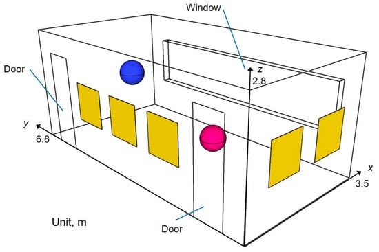
Figure 1.
Problem 1 for scalability test: a meeting room model. Blue and magenta spheres respectively represent the source point and the receiving point.
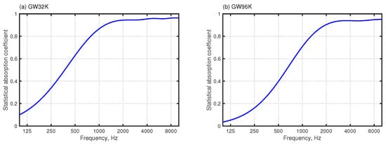
Figure 2.
Statistical absorption coefficient for (a) GW32K and (b) GW96K.
Figure 3 shows an analyzed model for Problem 2, which simulates acoustics in a classroom of 189 m with eight long desks and a platform. Problem 2 has larger dimensions and more complex geometry than Problem 1. A source point and a receiver are placed, respectively, at positions (x, y, z) = (0.5, 3.5, 1.5) and (2.8, 2.0, 1.2). The absorbing condition is the same as that used in Problem 1: ceiling—GW32K; absorbing panel (yellow surfaces in Figure 3)—GW96K; doors and windows—statistical absorption coefficient of 0.05; other surfaces—statistical absorption coefficient of 0.08.
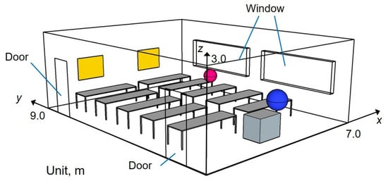
Figure 3.
Problem 2 for scalability test: classroom model. Blue and magenta spheres respectively represent the source point and the receiving point.
3.2. Computation Setting and Evaluation Index
Both room models were spatially discretized with uniform cubic-shaped eight-node elements with 0.0125 m edge length. The resulting FE meshes have 34,832,384 elements and 35,179,305 DOFs for Problem 1, and 97,069,568 elements and 97,917,391 DOFs for Problem 2. Problem 2 has about 2.8 times larger problem size. For both models, RIRs were calculated up to 1 s with . As an excitation signal for the sound source, the impulse response of the FIR filter with an upper-limit frequency of 6 kHz, created using the Parks–McClellan algorithm, was employed. The following speed-up index S used to evaluate the parallel performance of the solver was defined as
where is the computational time consumed for the case using X computational nodes, and where is the computational time consumed using b computational nodes as a baseline. The maximum number of computational node X is 64. Because one node has 96 CPU-cores, we use 6144 CPU-cores for X = 64. The measure S represents how the solver speeds up when using X nodes against the baseline. For Problem 1 and Problem 2, we set b to 1 and 2, respectively. The reason for for Problem 2 is the memory limitation on a node, i.e., in Problem 2, single node parallelization consumes the memory that exceeds 384 GBytes because of storage of information of the whole model on a node in addition to the global boundary condition matrix assembling in each process. We evaluated the parallel performance of the wave-based solver in two computational parts. One is the parallel performance of the time-marching scheme part, i.e., Equations (10)–(19), which is the main operation of the solver. Another is that, of all computational parts, which includes matrix construction parts as well as the time-marching scheme part. Parallel performance was verified up to 64 nodes while doubling the number of computation nodes. Metis library [28] was used to create subdomain meshes that achieve an even workload among the subdomains. Regarding the workload balance, Figure 4 shows coefficients of variance in DOFs and communication data per communication via MPI among computational processes in each parallel condition. The deviations in DOFs are very small: less than 3%. The coefficients of variance in communication data are around 20%. This is not a severe deviation. We therefore infer that the workloads of all subdomain meshes are well balanced.
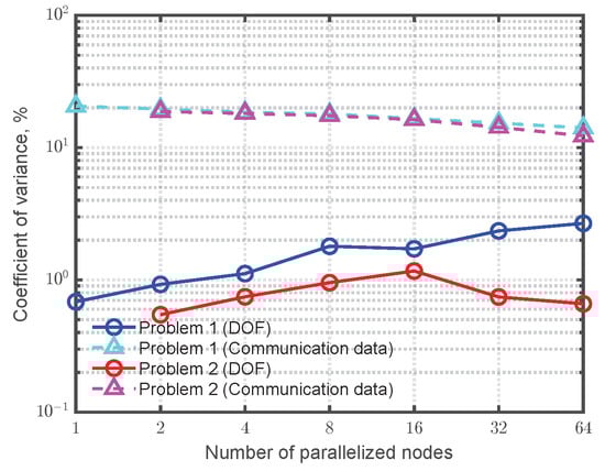
Figure 4.
Coefficients of variance for distribution of DOF and communication data per communication among all subdomains for each parallel condition.
3.3. Results and Discussion
First, we show how fast the present parallel wave-based solver enables us to compute room acoustics. Figure 5a presents the computational times for Problems 1 and 2 when using 1–64 nodes with the cloud HPC environment. For each problem, the results show the computational times on the time-marching scheme part (Time-marching) and all computational parts (Total). The wave-based solver presents a marked computational performance for both problems. The total computational times are only 217 s and 613 s for Problem 1 and Problem 2 when using 64 nodes. The computational time of Problem 2 is about 2.8 times longer than that of Problem 1. The computational time ratio corresponds to the ratio of the problem size. The wave-based solver is practical even using the baseline node: The computational times are 10,360 s and 14,555 s, respectively, for Problems 1 and 2. Additionally, the computational times of the time-marching scheme part and all computational parts are almost identical up to the use of 16 nodes. The computational time difference between the time-marching scheme and all computational parts is visible when using 32 and 64 nodes. The current code of the parallel solver loads a surface element mesh file by all computation processes simultaneously. It causes conflict among processes and delays in file loadings. Resolving the conflict is an issue that demands future study.
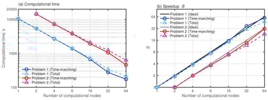
Figure 5.
Results of scalability tests of (a) computational time and (b) speedup S.
Figure 5b presents the speedup S in both problems, including ideal speedup values evaluated as . For both problems, the speedups in the time-marching scheme parts increase linearly, fitting well to the ideal S. When using 64 nodes, the speedup values for Problems 1 and 2 are, respectively, 59.7 and 31.5, which are close to their ideal values of 64 and 32. On the other hand, speedups on all computational parts were, respectively, 47.8 and 23.1 for Problems 1 and 2 when using 64 nodes because of the conflict in surface element mesh loading explained above. Although the conflict engenders slight performance reduction, the parallel performance remains high. We conclude that the present parallel wave-based solver which uses a cloud HPC environment is an effective and practical room-acoustics simulation tool.
4. Binaural Room-Acoustics Auralization in a Large-Scale Auditorium
This section describes potential of the proposed binaural auralization method with the parallel wave-based solver for a vast auditorium model of 745,335,325 DOF. This demonstration shows how the auditory impression of room-acoustics changes with the difference in acoustic treatments, presenting the importance of suppressing flutter echoes with sound absorbers for better speech clarity. We also present examples of the resulting Ambisonics signals, receivers’ directivities, acoustics parameters, and BRIRs, which present the plausibility of the proposed method.
4.1. Analyzed Model and Computation Setting
Figure 6 presents the auditorium model for demonstration: 2271 m with a source point (blue sphere) and six receivers (magenta spheres). The source is located at (x, y, z) = (2.1, 0, 1.2) and the locations of the receivers are listed in Table 2. We calculated BRIRs, including frequency components up to 5 kHz for two acoustic treatment cases, respectively designated as Cond. 1 and Cond. 2. The first uses the following acoustic treatment as a baseline: rigidly backed glass wool absorbers of 24 kg/m with 50 mm thickness (GW24K) were installed on the ceiling. In addition, GW-backed microperforated panels (MPPGW) were attached for the back wall, which also uses GW24K. For the audience seat area, rigidly backed needle felt (NF) with 15 mm thickness was installed. Other boundaries were treated as reflective materials having a statistical absorption coefficient of 0.175. The latter, Cond. 2, has further installed additional GW24K to side walls to suppress flutter echoes caused by multiple reflections between side walls. Other configuration details are the same as those of the baseline. The GW24K, MPPGW, and NF were modeled by the frequency-dependent impedance BCs, whereas other reflective materials were modeled by real-valued frequency-independent impedance BCs. We calculated the acoustic admittance of sound absorbers for frequency-dependent impedance BCs by the transfer matrix method [33], where the acoustical characteristics of GW24K and NF were modeled, respectively, using the Miki model [34], respectively assuming the flow resistivity of 6900 Pa s/m and 10,000 Pa s/m. In addition, MPP was modeled with the Maa model [35], considering 0.5 mm panel thickness, 0.5 mm hole diameter, a perforation ratio of 0.55 %, and dynamic viscosity of the air of 17.9 Pa s. The resulting acoustic admittance was fitted further with a multi-pole model with and for GW24K, , and for NF and and for MPP-GW. Detailed parameters of the multi-pole models are reported in the relevant literature [9]. Figure 7 presents statistical absorption coefficients for three absorbers: GW24K, MPPGW, and NF. Figure 8 also presents a comparison of average absorption coefficients of auditorium between two absorption conditions. Cond. 2 is associated with higher absorption coefficients than those of Cond. 1 at 250 Hz and higher by virtue of the additional absorption treatment on the side walls.
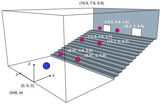
Figure 6.
Auditorium model for demonstrating binaural auralization application. Blue and magenta spheres respectively represent a source point and receiving points.
Table 2.
Locations of receivers in the auditorium model.
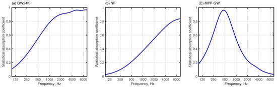
Figure 7.
Statistical absorption coefficients: (a) GW24K; (b) NF; and (c) MPP-GW.
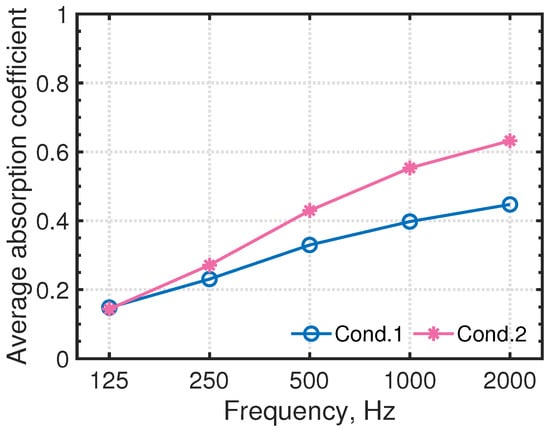
Figure 8.
Average absorption coefficients of the auditorium for two absorption conditions.
The impulse response of an optimized FIR filter designed with the Parks–McClellan algorithm having a flat spectrum from 80 Hz to 5 kHz was used as a sound source signal. Its waveform and spectrum are presented in Figure 9. This source signal is beneficial for evaluating acoustic parameters and auralization purposes compared to a well-used Gaussian pulse having a non-flat spectrum. The auditorium model was spatially discretized by various-sized 8-node hexahedral FEs having edge lengths of less than 0.015 m. The resulting FE mesh has 742,561,152 elements and ensures spatial resolution of 4.6 elements per wavelength at 5 kHz. A theoretical estimation shows the FE mesh can keep dispersion error of less than 1% [9]. After meshing, the computational model is divided into 6144 subdomains by partitioning software Metis [28]. Regarding the reference, the coefficients of variance in DOFs and communication data among subdomains were 0.3% and 11.8%, respectively. Then, the massively parallel wave-based computation was performed with 6144 CPU cores under the same cloud computing environment as that described in Section 3 to simulate the auditorium room acoustics.
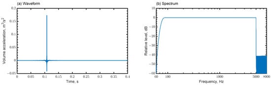
Figure 9.
Source signal: (a) waveform and (b) spectrum.
Consideration of Air Absorption
For accurate room-acoustics simulation of large spaces up to high frequencies, including the air absorption effect is crucially important. It is possible to account for air absorption because of viscothermal effects using the Stokes equation [7] instead of the lossless linear wave equation of Equation (1). In addition, there exists a model accompanying the relaxation effect [36]. In addition, a simple method of adding air absorption to simulated impulse responses from a lossless wave equation or geometrical acoustics models is also proposed, using a low-pass filter approximating the air absorption property. The present demonstration uses the time-varying low-pass IIR filter [37] to include air absorption in simulated RIRs under atmospheric conditions of 25 C and relative humidity of 50%.
4.2. Objective Analysis of Auditorium Room Acoustics
This section presents objective room-acoustics analysis results for the auditorium. Before presenting the results of such an analysis, we first present the practicality of the present massively parallel wave-based solver to large-scale room-acoustics simulation from computational cost aspects. The present massively parallel wave-based solver achieved remarkable computational speed, with computational times of 12,777 s and 12,028 s, respectively, for Cond. 1 and Cond. 2.
Furthermore, we show room-acoustics evaluation findings related to acoustic disturbance and receiver’s directivity in early and late time, using FOA signals. Figure 10a–d show simulated FOA signals at a receiver R3 of Cond. 1. Here, is the omnidirectional component and , , and are the bidirectional components in y-, z-, and x-directions. A repetition of intense reflected sounds is apparent; it seems likely to promote flutter echoes in because of the low absorptivity of the side walls. Figure 11a–d show FOA signals at R3 for Cond. 2 with additional sidewall sound absorbers. As shown in Figure 11b, adding sidewall sound absorbers decreases repetition of intense reflected sounds, thereby suppressing flutter echoes. The contribution of adding sidewall sound absorbers is also apparent for the other components. Naturally, the direct sound shows the largest amplitude for the component , which is the bidirectional component in the x-direction, compared to other components.
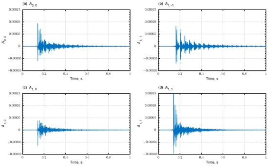
Figure 10.
Simulated FOA signals at R3 in Cond. 1: (a) ; (b) ; (c) ; and (d) .
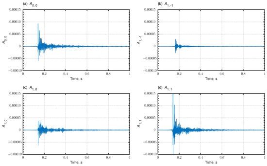
Figure 11.
Simulated FOA signals at R3 in Cond. 2: (a) ; (b) ; (c) ; and (d) .
Figure 12a–d further show the receiver’s horizontal directivity in early and late times at R3 and R4 for Cond. 1 and Cond. 2. The horizontal directivities are defined here as the summation of incident plane wave energy calculated using
where and are set to 0 and 50 ms for early time and 50 ms and ∞ for late time. Time 0 means the direct sound arriving time denoted in ISO3382-1 [38]. The horizontal case is calculated with . In addition, in Figure 12, and coincide with x-axis and y-axis directions. From this, for the receiver’s R3 and R4, the source respectively locates in directions of 180 and 202. It is apparent for the receiver R3 that early time directivities indicate the source location for both conditions, where s take the peak values at . In addition, the early directivities at R4 for both conditions present that their peak values track the sound source location corresponding to receiver location change from R3. Here, the peaks of s were found to be for Cond. 1 and for Cond. 2, which are slightly different directions of the exact source direction of 202 because the early time sounds at R4 include the reflected sound from the side wall located in the direction of . Cond. 2 presents better sound source localization than Cond. 1 by virtue of the installation of side wall absorbers. Effects of the side wall absorbers are also observed for both receivers because the incident energy decreases in both early and late directivities. Especially late directivities show a large effect by the added side wall absorbers. For Cond. 1, y directional components ( and ) are outstanding at both receivers. However, late directivities of Cond. 2 point to the source directions. Those FOA signal analysis results can be expected from the sound absorber configuration, demonstrating the feasibility of the present auditorium acoustics simulation.
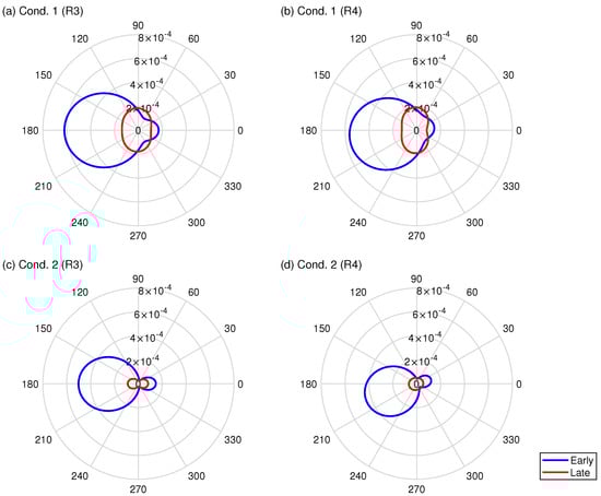
Figure 12.
Directivity patterns in early and late times on a horizontal plane against azimuth with the following absorption and receiver conditions: (a) Cond. 1 and R3; (b) Cond. 1 and R4; (c) Cond. 2 and R3; and (d) Cond. 2 and R4.
Figure 13a–d show four room-acoustics parameters, the reverberation time (T30), the early decay time (EDT), the A-weighted relative sound pressure level (SPL (A)), and the rapid speech transmission index (RASTI) at six receivers R1∼R6 for Cond. 1 and Cond. 2. Those parameters were evaluated using ODEON 16 room-acoustics simulation software with computed RIRs with the present wave-based solver. The reverberation times and EDT have averaged values greater than 500 Hz and 1 kHz. The reverberation times of both conditions show large differences, with spatially averaged values of 1.52 s for Cond. 1 and 0.93 s for Cond. 2. Their relative differences at each receiver are 35–45%. A large difference in EDT between both conditions is also notable. The spatially averaged EDT values are 0.96 and 0.64 in Cond. 1 and Cond. 2. The relative differences between Cond. 1 and Cond. 2 at the same receivers of 20–52% are much larger than the just notable difference (JND) of 5% [38]. From these results, we can infer that the auditory impression of auralized sounds, which comes from the additional side wall absorbers, shows a clear difference in reverberance. In addition, SPL(A) results show that SPL(A) becomes smaller for the receiver positions going in the back of the auditorium. For Cond. 1 and Cond. 2, SPL(A)s at R5 are −4.1 dB and −5.1 dB compared to those at R1. In addition, an SPL(A) comparison at the same receivers shows that SPL(A)s in Cond. 1 present more than 1 dB larger values than those of Cond. 2. The maximum difference is 2.3 dB at R6. A comparison of RASTI between both conditions shows that RASTI values in Cond. 2 take larger values more than JND value of speech transmission index of 0.03 [39] at all receivers than those of Cond. 1. The RASTI values are 54–58% in Cond. 1 and 56–65% in Cond. 2. We also expect distinct differences of speech clarity in auralized speech sounds between the two conditions.
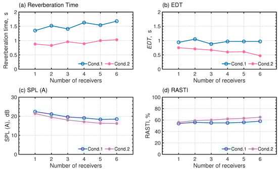
Figure 13.
Acoustic parameter: (a) reverberation time; (b) EDT; (c) SPL (A); and (d) RASTI.
Figure 14 presents a comparison of frequency characteristics of spatially averaged reverberation time and EDT with the Eyring–Knudsen formula. The error bars in numerical results show their standard deviations. The Eyring–Knudsen formula values and T30 values differ except for Cond. 1 at 125 Hz, indicating low diffusivity of sound fields. In Cond. 1, T30 becomes larger with frequencies above 500 Hz, whereas the average absorption coefficient decreases with frequency. The frequency characteristic of Cond. 2’s T30 shows the same tendency as the average absorption coefficient because of cancellation of the flutter echo with the additional absorber. Moreover, EDT values agree with the Eyring–Knudsen formula, which is better than T30 except for Cond. 1 at 125 Hz. The result indicates that the wave-based room-acoustics solver accurately models frequency-dependent absorption characteristics of boundary surfaces.
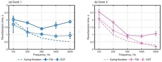
Figure 14.
Comparisons of reverberation properties in the auditorium calculated using the Eyring–Knudsen formula and the wave-based solver: (a) Cond. 1 and (b) Cond. 2.
We present examples for BRIRs calculated with FOA signals and HRIR at R3 and R4 for Cond. 1 in Figure 15. The BRIRs are calculated after rotating FOA signals so that the front of a listener is in . Consequently, direct sound arrives from the front at R3, whereas it comes from the left obliquely forward at R4. Such differences in directions of direct sound arrival are confirmed from BRIRs where direct components of and at R3 are of the same magnitude, whereas at R4 presents larger amplitude than . The result also reinforces the plausibility of the present auditorium acoustics simulation. Additionally, there are repeated intense reflections in both BRIRs. We can expect to perceive flutter echoes at receivers R3 and R4 in Cond. 1.
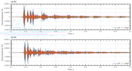
Figure 15.
BRIRs for Cond. 1 at (a) R3 and (b) (R4).
4.3. Binaural Room-Acoustics Auralization
As Supplemental Materials, we provide binaural audible files of simulated BRIRs and signals convoluted with speech in Japanese and English at each receiver in Cond. 1 and Cond. 2 (can be downloaded at https://www.mdpi.com/article/10.3390/app13052832/s1). Dry sources of Japanese and English speeches were collected in sound material in living environment 2004 (SMILE 2004) [40]. For all receivers, the front is set in the direction of the x-axis. One would perceive the difference in horizontal source direction between the receivers pair on the same lines in the y-direction for both conditions. Additionally, for BRIRs of Cond. 1, flutter echoes can be heard clearly at all receivers with longer reverberation than Cond. 2. In contrast, flutter echoes are not perceived in Cond. 2 at all receivers because of the effects of the added side wall absorbers. Differences in reverberation between both conditions are also experienced for speech sounds. Regarding the loudness, for example, sounds become smaller at R5, which is located far from the sound source, compared to R1. RASTI and perceived speech clarity also respond well. Actually, Cond. 2 presents clearer sounds than Cond. 1 for the same receiver comparison. This is especially true for speech sounds at receiver R6, where Cond. 2 takes the maximum RASTI value and presents a distinct difference in speech clarity between the two conditions. The results demonstrated clearly the potential of the proposed binaural room-acoustics auralization method.
5. Conclusions
The proposed binaural room-acoustics auralization method uses a highly scalable wave-acoustics-based solver that is applicable to large-scale room-acoustics problems under a cloud HPC environment. The binaural room-acoustics auralization is based on a hybrid technique using Ambisonics and HRTF. The Ambisonics encoding uses room impulse responses computed using a wave-based solver based on dispersion-optimized explicit TD-FEM. Detailed procedures of computing expansion coefficients of spherical harmonics using spatial differentiation of shape function of FEs are also proposed.
This paper first presented examination of the scalability of the present parallel wave-based solver on an HPC cloud environment to address the question of solver efficiency when computing room impulse responses for practical room-acoustics problems. Two room-acoustics problems with different problem sizes and geometrical complexities were selected: a meeting room-acoustics simulation and a classroom-acoustics simulation. The parallel performance examination involved using up to 6144 CPU cores on the HPC cloud environment and computing room impulse responses, including frequency components up to 6 kHz. Results showed that the present parallel wave-based solver is an efficient means of simulating room acoustics under the HPC cloud environment. It can compute room impulse responses rapidly. It was possible to compute room impulse responses with 217 s for a meeting room having 35,00,000 DOFs when using 6144 CPU cores. For a classroom problem having 100,000,000 DOFs, the computational time was only 613 s. Results also demonstrated the high scalability of the present parallel wave-based solver. The speedup increased almost linearly with an increasing number of CPU cores used.
Next, we demonstrated the potential of the proposed binaural room-acoustics auralization method via an auditorium acoustics simulation up to 5 kHz having 750,000,000 DOFs. This problem size is the largest ever reported for an architectural acoustics problem with FEM-based room-acoustics solvers. By this simulation, we demonstrated how room acoustics change with two acoustics treatments: The first treatment produces flutter echoes. Another is an acoustic treatment suppressing flutter echoes with additional sound absorbers installed on side walls. The plausibility of the proposed binaural room-acoustics auralization method was first demonstrated by comparing the first-order Ambisonics signals, the receiver’s directivity, and four room acoustical parameters between the two conditions. The findings indicated behavior consistent with those expected from the two acoustic treatments. In addition, the binaural room-acoustics auralization showed that auditory impression corresponds to the objective analysis. It is also notable that the parallel wave-based solver can simulate the room acoustics of this huge model within 13,000 s using 6144 cores.
As a subsequent stage of the present study, we expect to examine the proposed binaural auralization method with measurements, with expansion to high-order Ambisonics.
Supplementary Materials
The following supporting information can be downloaded online. We supply the audio data (.WAV files) explained in Section 4.3 as supplemental materials where BRIRs, Japanese, and English speeches at all receivers in two absorption conditions are arranged. Those can be downloaded at: https://www.mdpi.com/article/10.3390/app13052832/s1. Specifically, we provide a zip file for which the first level comprises three folders: “brir”, “japanese” and “english”; the second comprises two absorption conditions: “condition 1” and “condition 2”, and the last level with receiver names R1–R6.
Author Contributions
Conceptualization, T.Y.; Funding acquisition, T.O.; Investigation, T.Y.; Methodology, T.Y.; Project administration, K.S.; Resources, T.O.; Software, T.Y. and T.O.; Supervision, T.O.; Validation, T.Y.; Visualization, T.Y.; Writing—original draft, T.Y. and T.O.; Writing—review and editing, T.Y., T.O. and K.S. All authors have read and agreed to the published version of the manuscript.
Funding
This work was supported in part by a Kajima Foundation Scientific Research Grant.
Institutional Review Board Statement
Not applicable.
Informed Consent Statement
Not applicable.
Data Availability Statement
The raw data supporting the conclusions presented in this report will be made available by the corresponding author on request.
Acknowledgments
The authors wish to thank Shiho Kusabiraki, Takashi Ogawa, Takuya Iseda and Taro Miyazaki from AWS Japan for their kind help with construction of the cloud HPC environment.
Conflicts of Interest
The authors declare that they have no conflict of interest.
References
- Vorländer, M. Auralization: Fundamentals of Acoustics, Modelling, Simulation, Algorithms and Acoustic Virtual Reality; Springer Science & Business Media: Berlin/Heidelberg, Germany, 2007. [Google Scholar]
- Sakuma, T.; Sakamoto, S.; Otsuru, T. (Eds.) Computational Simulation in Architectural and Environmental Acoustics: Methods and Applications of Wave-Based Computation; Springer: Tokyo, Japan, 2014. [Google Scholar]
- Savioja, L.; Svensson, U.P. Overview of geometrical room acoustic modeling techniques. J. Acoust. Soc. Am. 2015, 138, 708–730. [Google Scholar] [CrossRef]
- Okuzono, T.; Otsuru, T.; Tomiku, R.; Okamoto, N.; Minokuchi, T. Speedup of time domain finite element sound field analysis of rooms. In Proceedings of the 37th International Congress and Exposition on Noise Control Engineering, Shanghai, China, 26–29 October 2008. [Google Scholar]
- Saarelma, J.; Savioja, L. An open source finite-difference time-domain solver for room acoustics using graphics processing units. In Proceedings of the Forum Acusticum 2014, Krakow, Poland, 7–12 September 2014. [Google Scholar]
- Morales, N.; Mehra, R.; Manocha, D. A parallel time-domain wave simulator based on rectangular decomposition for distributed memory architectures. Appl. Acoust. 2015, 97, 104–114. [Google Scholar] [CrossRef]
- Hamilton, B.; Webb, C.J.; Fletcher, N.; Bilbao, S. Finite difference room acoustics simulation with general impedance boundaries and viscothermal losses in air: Parallel implementation on multiple GPUs. In Proceedings of the International Symposium on Musical and Room Acoustics ISMRA 2016, La Plata, Argentina, 11–13 September 2016. [Google Scholar]
- Morales, N.; Chavda, V.; Mehra, R.; Manocha, D. MPARD: A high-frequency wave-based acoustic solver for very large compute clusters. Appl. Acoust. 2017, 121, 82–94. [Google Scholar] [CrossRef]
- Yoshida, T.; Okuzono, T.; Sakagami, K. A Parallel Dissipation-Free and Dispersion-Optimized Explicit Time-Domain FEM for Large-Scale Room Acoustics Simulation. Buildings 2022, 12, 105. [Google Scholar] [CrossRef]
- Yoshida, T.; Okuzono, T.; Sakagami, K. Dissipation-free and dispersion-optimized explicit time-domain finite element method for room acoustic modeling. Acoust. Sci. Technol. 2021, 42, 270–281. [Google Scholar] [CrossRef]
- Berkhout, A.J.; de Vries, D.; Vogel, P. Acoustic control by wave field synthesis. J. Acoust. Soc. Am. 1993, 93, 2764–2778. [Google Scholar] [CrossRef]
- Ise, S. A principle of sound field control based on the Kirchhoff–Helmholtz integral equation and the theory of inverse systems. Acta Acust. United Acust. 1999, 85, 78–87. [Google Scholar]
- Gerzon, M.A. Periphony: With Height Sound Reproduction. J. Audio Eng. Soc. 1972, 21, 2–10. [Google Scholar]
- Daniel, J.; Moreau, S.; Nicol, R. Further Investigations of High-Order Ambisonics and Wavefield Synthesis for Holophonic Sound Imaging. In Proceedings of the 114th Audio Engineering Society Convention, Amsterdam, The Netherlands, 22–25 March 2003. [Google Scholar]
- McKenzie, T.; Murphy, D.T.; Kearney, G. Interaural Level Difference Optimization of Binaural Ambisonic Rendering. Appl. Sci. 2019, 9, 1226. [Google Scholar] [CrossRef]
- Otani, M.; Shigetani, H.; Mitsuishi, M.; Matsuda, R. Binaural Ambisonics: Its optimization and applications for auralization. Acoust. Sci. Technol. 2020, 41, 142–150. [Google Scholar] [CrossRef]
- Llopis, H.S.; Pind, F.; Jeong, C.-H. Development of an auditory virtual reality system based on pre-computed B-format impulse responses for building design evaluation. Build. Environ. 2020, 169, 106553. [Google Scholar] [CrossRef]
- Doggett, R.; Sander, E.J.; Birt, J.; Ottley, M.; Baumann, O. Using Virtual Reality to Evaluate the Impact of Room Acoustics on Cognitive Performance and Well-Being. Front. Virtual Real. 2021, 2, 620503. [Google Scholar] [CrossRef]
- Cirillo, E.; Martellotta, F. Sound propagation and energy relations in churches. J. Acoust. Soc. Am. 2005, 118, 232–248. [Google Scholar] [CrossRef] [PubMed]
- Merimaa, J.; Pulkki, V. Spatial impulse response rendering I: Analysis and synthesis. J. Audio Eng. Soc. 2005, 53, 1115–1127. [Google Scholar]
- Shimokura, R.; Soeta, Y. Sound field characteristics of underground railway stations: Effect of interior materials and noise source positions. J. Acoust. Soc. Am. 2012, 73, 1150–1158. [Google Scholar] [CrossRef]
- Yoshida, T.; Ueda, Y.; Mori, N.; Matano, Y. An Experimental Study of the Performance of a Crossed Rib Diffuser in Room Acoustic Control. Appl. Sci. 2021, 11, 3781. [Google Scholar] [CrossRef]
- Okuzono, T.; Yoshida, T.; Sakagami, K. Efficiency of room acoustic simulations with time-domain FEM including frequency-dependent absorbing boundary conditions: Comparison with frequency-domain FEM. Appl. Acoust. 2021, 182, 108212. [Google Scholar] [CrossRef]
- Okuzono, T.; Yoshida, T. High potential of small-room acoustic modeling with 3D time-domain finite element method. Front. Built Environ. 2022, 8, 1006365. [Google Scholar] [CrossRef]
- Dragna, D.; Pineau, P.; Blanc-Benon, P. A generalized recursive convolution method for time-domain propagation in porous media. J. Acoust. Soc. Am. 2015, 138, 1030–1042. [Google Scholar] [CrossRef] [PubMed]
- Zienkiewicz, O.C.; Taylor, R.L.; Zhu, J.Z. The time dimension: Semi-discretization of field and dynamic problems. In The Finite Element Method: Its Basis and Fundamentals, 7th ed.; Butterworth–Heinemann: Oxford, UK, 2013; pp. 382–386. [Google Scholar]
- Yoshida, T.; Okuzono, T.; Sakagami, K. Numerically stable explicit time-domain finite element method for room acoustics simulation using an equivalent impedance model. Noise Control Eng. J. 2018, 66, 176–189. [Google Scholar] [CrossRef]
- Karypis, G.; Kumar, V. A Fast and Highly Quality Multilevel Scheme for Partitioning Irregular Graphs. SIAM J. Sci. Comput. 1999, 20, 359–392. [Google Scholar] [CrossRef]
- Zotter, F.; Frank, M. Ambisonics: A Practical 3D Audio Theory for Recording, Studio Production, Sound Reinforcement, and Virtual Reality; Springer: Cham, Switzerland, 2019. [Google Scholar]
- Sheaffer, J.; van Walstijn, M.; Rafaely, B.; Kowalczyk, K. Binaural Reproduction of Finite Difference Simulations Using Spherical Array Processing. IEEE/ACM Trans. Audio Speech Lang. Process. 2015, 23, 2125–2135. [Google Scholar] [CrossRef]
- Bilbao, S.; Politis, A.; Hamilton, B. Local Time-Domain Spherical Harmonic Spatial Encoding for Wave-Based Acoustic Simulation. IEEE Signal Process. Lett. 2019, 26, 617–621. [Google Scholar] [CrossRef]
- Politis, A. Microphone Array Processing for Parametric Spatial Audio Techniques. Ph.D. Thesis, Aalto University, Helsinki, Finland, 2016. [Google Scholar]
- Allard, J.F.; Atalla, N. Acoustic impedance at normal incidence of fluids. Substitution of a fluid layer for a porous layer. In Propagation of Sound in Porous Media: Modeling Sound Absorbing Materials, 2nd ed.; John Wiley & Sons: Chichester, UK, 2009; pp. 15–27. [Google Scholar]
- Miki, Y. Acoustical properties of porous materials – Modification of Delany–Bazley models. J. Acoust. Soc. Jpn. (E) 1990, 11, 19–24. [Google Scholar] [CrossRef]
- Maa, D.-M. Microperforated-panel wideband absorbers. Noise Control Eng. J. 1987, 29, 77–84. [Google Scholar] [CrossRef]
- Hamilton, B.; Bilbao, S. Time-domain modeling of wave-based room acoustics including viscothermal and relaxation effects in air. JASA Express Lett. 2021, 1, 092401. [Google Scholar] [CrossRef]
- Kates, J.M.; Brandewie, E.J. Adding air absorption to simulated room acoustic models. J. Acoust. Soc. Am. 2020, 148, EL408–EL413. [Google Scholar] [CrossRef]
- ISO. 3382–1:2009; Acoustics—Measurement of Room Acoustic Parameters—Part 1: Performance Spaces. International Organization for Standardization (ISO): Geneva, Switzerland, 2009.
- Bradley, J.S.; Reich, R.; Norcross, S.G. A just noticeable difference in C50 for speech. Appl. Acoust. 1999, 58, 99–108. [Google Scholar] [CrossRef]
- Kawai, K.; Fujimoto, K.; Iwase, T.; Sakuma, T.; Hidaka, Y.; Yasuoka, H. Introduction of sound material in living environment 2004 (SMILE 2004): A sound source database for educational and practical purposes. J. Acoust. Soc. Am. 2006, 120, 3070–3071. [Google Scholar] [CrossRef]


Disclaimer/Publisher’s Note: The statements, opinions and data contained in all publications are solely those of the individual author(s) and contributor(s) and not of MDPI and/or the editor(s). MDPI and/or the editor(s) disclaim responsibility for any injury to people or property resulting from any ideas, methods, instructions or products referred to in the content. |
© 2023 by the authors. Licensee MDPI, Basel, Switzerland. This article is an open access article distributed under the terms and conditions of the Creative Commons Attribution (CC BY) license (https://creativecommons.org/licenses/by/4.0/).