Abstract
Parallel hierarchical scheduling of multicore processors in avionics hypervisor is being studied. Parallel hierarchical scheduling utilizes modular reasoning about the temporal behavior of the upper Virtual Machine (VM) by partitioning CPU time. Directed Acyclic Graphs (DAGs) are used for modeling functional dependencies. However, the existing DAG scheduling algorithm wastes resources and is inaccurate. Decreasing the completion time (CT) of DAG and offering a tight and secure boundary makes use of joint-level parallelism and inter-joint dependency, which are two key factors of DAG topology. Firstly, Concurrent Parent and Child Model (CPCM) is researched, which accurately captures the above two factors and can be applied recursively when parsing DAG. Based on CPCM, the paper puts forward a hierarchical scheduling algorithm, which focuses on decreasing the maximum CT of joints. Secondly, the new Response Time Analysis (RTA) algorithm is proposed, which offers a general limit for other execution sequences of Noncritical joints (NC-joints) and a specific limit for a fixed execution sequence. Finally, research results show that the parallel hierarchical scheduling algorithm has higher performance than other algorithms.
1. Introduction
Multicore processors in avionics systems are being used to meet the increasing demands for performance and energy efficiency [1,2,3]. In the design of a real-time multi-core system, to avoid the interference of system resources, physical isolation technology is often used to isolate system resources. Virtualization technology can deploy subsystems with different functions on virtual machines running on the same hardware platform, which provides a more flexible method for system isolation and resource management. For virtual machines, the hypervisor is responsible for managing virtual machines and shielding the implementation details of the underlying hardware. Flexible strategies are adopted to effectively allocate the underlying hardware resources to virtual machines, to meet the resource requirements of every virtual machine. For real-time multi-core systems, virtualization technology can well meet some urgent requirements in the design of real-time multi-core systems. However, virtualization technology is still a new application direction in the field of real-time embedded systems, and the related research work is still very limited. The main problem is that when virtualization technology is introduced into real-time embedded systems, the response performance of real-time operating systems running on virtual machines is easily affected by the virtualization software layer. The semantic gap caused by the introduction of the virtualization layer makes it difficult for virtual machine monitors to perceive the application types of upper-level virtual machines. It hinders the virtual machine monitor from effectively allocating hardware resources according to the requirements of the upper application, thus it cannot provide a good guarantee for applications with high real-time requirements. Important research to ensure the quality of service is to dynamically allocate enough resources to the real-time VM and make it real-time.
When deploying a virtualization environment in avionics systems, the virtualization system needs to adopt a hierarchical scheduling framework. (i) Scheduling of VCPUs on PCPUs; (ii) Scheduling of real-time tasks in VCPUs (Figure 1) [4,5,6]. The scheduling levels at these two layers must meet the real-time guarantee, thus fulfilling the real-time guarantee of the whole system. However, classical real-time scheduling is no longer applicable to this hierarchical scheduling structure. A hierarchical scheduling framework needs to provide hierarchical resource sharing and allocation strategies for different scheduling services under different scheduling algorithms. The hierarchical scheduling framework can be expressed as a tree with a joint (hierarchical) structure. Every joint can be expressed as a scheduling model and the resources are to be allocated from the parent joint to the child’s joint. The resource allocation from the parent joints to the child’s joints can be regarded as a scheduling interface from the parent joint to the child. Therefore, the hierarchical real-time scheduling problem can be transformed into the schedulability analysis of the scheduling interfaces of the child and parent joints [7,8,9].
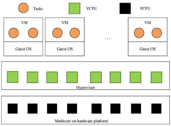
Figure 1.
Virtualization hierarchical scheduling framework.
To solve this problem, in recent years, some researchers have begun to pay attention to the parallel hierarchical scheduling of multicore processors. At present, most of the research on program parallelization in multi-verification focuses on the DAG task model [10]. DAG task model can describe the execution dependencies of task threads, such as parallel execution and serial execution. The sequential synchronous parallel task model is a stricter model for task behavior in the parallel DAG model. In this model, tasks can be divided into segments executed in series, every part can contain any number of parallel threads, and whole threads have to synchronize at the end of the segment. The existing DAG real-time task scheduling algorithms have two types: global scheduling and federated scheduling [11,12]. In global scheduling, multiple DAG tasks enjoy together whole multicores, so the overall resource utilization of the system may be high [5,6,7,8,9,10]. Due to complex interference between tasks, global scheduling has great inaccuracy. In federated scheduling, every task is assigned to some dedicated processors, where it can be executed without interference from other tasks. The scheduling analysis is relatively simple, but it wastes resources [12].
The main contribution: a single-cycle non-preemptive DAG task runs on an isomorphic multicore processor. By making full use of joint-level parallelism and inter-joint dependency, which are the essence of topology, they decrease the maximum CT and offer a tight and safe boundary for the maximum CT. This paper presents a new algorithm of the parallel hierarchical scheduling method that has two sections: (i) DAG parallel schedulability analysis, and (ii) hierarchical scheduling in the hypervisor.
The rest of this article is organized as follows. In Section 2, the system and task model are introduced. Section 3 describes the state-of-the-art approaches in DAG scheduling and analysis with a motivational example. The proposed scheduling method, CPCM, and the new response time analysis are explained in Section 4. The hierarchical scheduling in the hypervisor is provided in Section 5. Results are given in Section 6. Finally, Section 7 concludes this article.
2. Preliminaries
2.1. System Model
The system defines parallel task sets which are scheduled on a multi-core processor, the task set is defined as consisting of tasks , and the hardware platform includes homogeneous processors. Each task is represented by a DAG with joints and edges connecting these joints.
2.2. Task Model
Any DAG task is , where is the constrained relative deadline, is the minimum inter-arrival time, within , and is the graph defining a series of activities forming the task. The graph is characterized by where is a series of joints and is a series of directed edges connecting any two joints. Every joint is the computation unit that must be executed unceasingly and is defined by WCET (Worst Case Execution Time), namely .
Either , form a directional edge, only if has finished and begins to be executed, is a predecessor of , and is a successor of . Each joint has a and a , and . Joints that are either directly or transitively predecessors and successors of a joint are termed as its ancestors and descendants respectively. The joint with or is referred to as the sink or source . In order not to lose generality, suppose DAG has one sink and source joint. Joints that can execute concurrently with are given by [13].
DAG tasks have basic characteristics. Firstly, an arbitrary path is a joint sequence in V and follows . The path in V is defined as . A local path is a sub-path within the task and as such does not feature both the source and the sink , provides the length of . Secondly, the longest complete path is referred to as the critical path (CP) , and its length is denoted by , where . Joints in are referred to as the critical joints. Other joints are referred to as NC-joints (NC-joints), denoted as . Finally, the workload W is the sum of a task’s WCETs, . The workload of all NC-joints is called the non-critical workload.
Figure 2a depicts a DAG task with . The number in the upper left corner of every joint provides WCET, for example . For have , , and . L = 14, C = 30, , , .
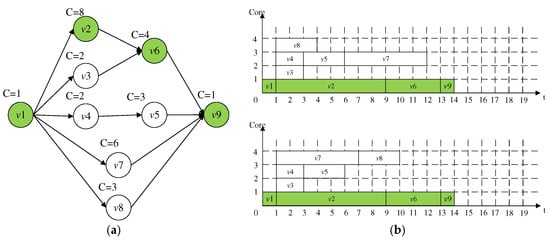
Figure 2.
Example of a DAG task; (a) A DAG task (b) Execution scene.
2.3. Work-Conserving Schedulability Analysis
When there is a pending workload, the scheduling algorithm never idles the processor, and it is called a work-conserving algorithm [14]. A general bound is provided, which catches the worst-case (WC) response time of globally scheduling tasks using any work-saving algorithm [15]. This analysis is then formalized in the DAG task in Formula (1) [16]. is the response time of , is the number of processors, is the interference from a high priority DAG task , and is whole high priority tasks of .
Figure 2b shows some execution scene of DAG in a quad-core processor. For casually scheduled joints, there may be a series of 420 execution scene, the maximum CT is less than 14, and gives . They take less than 18. Based on the above, the paper puts forward a new algorithm to decrease the makespan of the runtime.
3. Related Work
For multicore processors with global solutions, the existing scheduling methods aim to decrease the maximum CT and tighten analysis limit of the worst case. They can be divided into joint-based [17] or slice-based [18,19] methods. Chip-based scheduling implements joint-level preemption and divides every joint into many small computing units. The slice-based method can promote the joint-level parallelism, but to achieve an improvement, it is necessary to control the numeral of preemption and migration. The joint-based method provides a better general solution by generating a clear joint execution sequence based on heuristics derived from the spatial or temporal characteristics of DAG [20].
Two of the latest joint-based approaches are described below. An exception-free non-preemptive scheduling method for single-cycle DAG is proposed, which always executes the longest ready joint of WCET to improve the parallelism. This prevents an exception when a joint executes less than its WCETs, which will cause the execution order to be different from the plan. This is achieved by ensuring that the joints are executed in the same order as the offline simulation. However, if the dependency between joints is not considered, this scheduling cannot minimize the delay of DAG completion. This algorithm leads to a scene with a maximum CT of 14, in which the NC-joint prolongs DAG completion due to a delayed start in Figure 2.
A new Response Time Analysis (RTA) method is proposed, which is superior to the traditional method when the execution sequence of joints is known [16,17,18]. That is, joint can only lead to delays from concurrent joints scheduled before . A scheduling algorithm is given, in which (i) the CP is always executed first, and (ii) the first is always the intermediate interfering joint. The novelty lies in considering the topology and path length in DAG, and providing the analysis compared with our method [19,20]. However, the parallel joints are scheduled according to the length of the longest full path, and the joints in the longest full path are scheduled first. Heuristic algorithms do not rely on perception, which will decrease parallelism and thus prolong the final CP.
4. Schedulability Analysis
4.1. Scheduling
Formula (1) shows that minimizing the latency from NC-joints to CPs effectively decreases the maximum CT of DAG. To support this point, a CPCM is recommended to take full advantage of joint dependency and parallelism. A scheduling algorithm to maximize the parallelism of joints is proposed. This is achieved through rule-based priority allocation, in which rules are designed to statically assign priority to every joint: (i) Always give priority to the CP priority, (ii) Rule 2 and 3 to maximize parallelism, (iii) minimize the latency of the CP. The algorithm is universally applicable to DAG of any topology. It adopts homogeneous processors, but there is no limit to the number of processors [21,22,23].
4.1.1. Concurrent Parent and Child Model
The CPCM includes two key parts. (i) The CP is divided into a set of consecutive sub-paths based on the potential delay that can happen (in Figure 3a). (ii) With every sub-path, CPCM distinguishes NC-joints, which can run in parallel with the sub-path and prolong the start of the next sub-path on the basis of priority constraints (in Figure 3b,c).
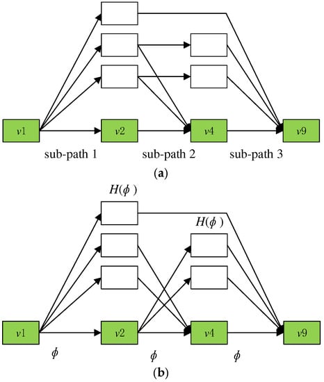
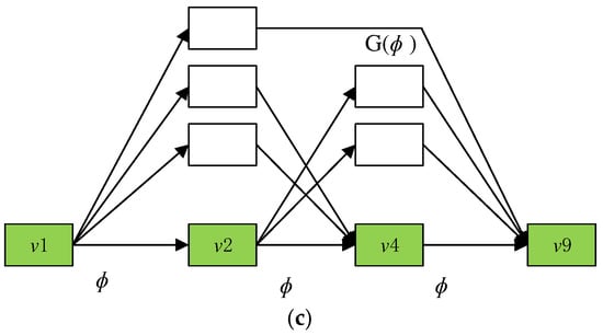
Figure 3.
The CPCM of a DAG. (a) the CP is divided into a set of consecutive sub-paths based on the potential delay it can incur. (b) execute in parallel with the sub-path. (c) delay the start of the next sub-path, based on precedence constraints.
The intuition of the CPCM is: when the critical path is executing, it utilizes just one core so that the non-critical ones can execute in parallel on the remaining cores. The time allowed for executing non-critical joints in parallel is termed as the capacity, which is the length of the critical path. Note that non-critical joints that utilize this capacity to execute cannot cause any delay to the critical path. The sub-paths in the critical path are termed capacity parents and all non-critical joints are capacity children . For each parent , it has a set of children that can execute using ’s capacity as well as delay the next parent in the critical path.
Algorithm 1 shows the process for constructing the CPCM. Starting from the scratch in , capacity parents are formed by analyzing joint dependency between the CP and NC-joints. A parent , its joints should run consecutively without prolong from NC-joints according to dependency. Every joint in , other than the scratch, only owns a predecessor which is the previous joint in . Three capacity parents are identified in Figure 3b.
| Algorithm 1: Concurrent Parent and Child Model algorithm |
| Input: Output: Specifications: |
| if /* distinguishing capacity parents */ for every |
| while do end end /* distinguishing capacity children */ for every end return |
Every , its children are determined to the joints that can run synchronously to , and prolong the start of . Joints in that finish after will prolong the start of . Joints in can prolong if they are finished later than in Figure 3b. The CPCM shows details of the possible latency attributed to NC-joints on the CP.
In addition, a child can start before, synchronized with, or after the start of . With the latter two, they will just use the capacity of . Children of earlier releases can run at the same time as some previous parents, thus interfering with their children and causing indirect delays to parents. With a parent , is the joints that fall within the child groups of later parents, but which can run with in parallel. Joints in , fall within , in Figure 3c. However, on the basis of the precedence constraints, it can be executed in parallel with and respectively.
Using the CPCM, the DAG is converted to a series of capacity parents and children, is time complexity. The CPCM supplies complete information about possible delays of NC-joints on the CP. Every parent , joints in can use a capacity of on every of processors to run in parallel as lead, storing possible latency.
Reanalyze in Figure 2a, the CP has three parents , and , as the delay from the NC-joint just appears at the header of the parents. For every parent, , and . In short, whole joints in can start before prolonging the execution of and the start of . , .
Parallel and disruptive workloads of the capacity parent are now formalized. is the completion time of a parent or a child joint , , is the length and the total workload of is , and . The terms parallel and disruptive workload of a parent is formally defined. as a child can be accounted for more than once if it can run concurrently with multiple parents.
Definition 1.
The parallel workloadofis the workload inthat can run starting at the time instant.
Definition 2.
The interfering workload ofis the workload inthat runs after the time instant. With a parent, its interfering workload is.
Theorem 1.
For parentsand, the workload inthat can prolong the start ofisat best.
Proof.
Based on the CPCM, the start of depends on the finish of both and , which is . By Definition 1, will not cause any delay as it always finishes before , and hence, the Theorem follows. Note that, although cannot delay directly, it can delay on nodes in , and in turn, causes an indirect delay to . □
4.1.2. The CP Priority Execution (CPPE)
The CP is regarded as a series of capability parents. It can be safely said that every full path could be regarded as the parents, which provides the time interval of its path length for other joints to run in parallel. However, since the CP offers the maximum capacity, the maximum total parallel workload can be achieved. It offers the basis for minimizing the disturbing workload on the whole CP.
Theorem 2.
For a schedulewith CPPE and a schedulethat prioritizes a random complete path over the CP, the total parallel workload of parents in S is always equivalent to or higher than that of,.
Proof.
First, suppose the length of parent is shortened by ∆ after the change from to . The same reduction applies on its finish time, i.e., . Because nodes in are shortened, the finish time of a child node can also be reduced by a value from (i.e., a reduction on ’s interference, if all the shortened nodes in belong to ) to ∆ (if all such nodes belong to ). By Definition 1, a child can contribute to the if or . Therefore, cannot increase in , as the reduction on (i.e., ∆) is always equal or higher than that of (i.e., or ∆).
Second, let and denote the length of the parent path under and (with ), respectively. The time for non-critical nodes to execute in parallel with the parent path is on each of m − 1 cores under . Thus, a child path with its length increased from to directly leads to an increase of in the interfering workload, as at most in the child can execute in parallel with the parent.
Therefore, both effects cannot increase the parallel workload after the change from to , and hence, . □
Rule 1.
.
4.1.3. Exploiting Parallelism and Joint Dependency
Using CPPE, the next goal is to maximize the parallelism of NC-joints and decrease latency of CP completion. On the basis of the CPCM, every parent correlates with , . With , it could run before and use the capacity of to run, if a high priority is assigned. In this instance, prolongs the finish of and the start of , squanders the capacity of its parent. Similar results are also acquired, which avoid this latency by first probing the front interfering joints.
Rule 2.
.
Consequently, a second allocation Rule is derived to rule the priority of every parent in the child groups. With any two neighboring parents and , the priority of any child in is higher than the children in . The latency from on can be minimized, because whole joints in fall within children of following parents and are always assigned with a lower priority than joints in in Rule 2.
Scheduling the child joints in every , concurrent joints with the same lead time are sorted by the length of their longest full path. Nevertheless, on the basis of CPCM, a full path can be divided into some partial paths, and all of these partial paths fall within a subgroup of different parents. With partial paths in , the order of their lengths can be completely reversed from to the order of their full paths. Therefore, this method can prolong the end time of .
In the constructed scheduling, it is guaranteed to assign higher priority to the longer local paths in a dependency-aware way. It will result in the final allocation rule. Symbol is the length of the longest local path in that contains . This length can be calculated by traversing in , such as in Figure 2, , , so is assigned a higher priority than . Rules 1–3 are applied to the sample, and the better-case schedule with a maximum full-time of 14 is finally obtained.
Rule 3.
.
Nevertheless, applying Rule 3 to every is not enough. Given the DAG structure, every can form a smaller DAG , and an inner nested CPCM with the longest path in is the parent. In addition, this process can be applied recursively to build an internal CPCM for every subgroup in the nested CPCM until whole local paths in the subgroup are completely absolute. With every internally CPCM, Rules 1 and 2 should be applied to maximize the capacity and minimize the latency of every subgroup, while Rule 3 is applied only to the independent paths in subgroups to maximize parallelism. This makes complete dependencies between joints and ensures that the longest path in every nested CPCM takes precedence.
Algorithm 2 shows the method of priority allocation based on Rule. The approach starts from the outer-most CPCM , assign the highest priority to whole parent joints according to Rule 1. In accordance with Rule 2, it starts from before and searches for the longest local path in . If there exists a dependency between nodes in and , is further constructed as an inner CPCM with the assignment algorithm applied recursively. This resolves the detected dependency by dividing into a set of providers. Otherwise, is an independent local path so that priority is assigned to its nodes based on Rule 3. The algorithm then continues with . The process goes on until whole joints in V are assigned priority.
| Algorithm 2: Priority assignment algorithm |
| Input: Output: Parameter: Intialise: |
| /* Rule 1. */ /* Rule 2. */ for every , do while do |
| /* Seek for the longest partial path in . */ |
| : if then break else /* Rule 3. */ end end end |
Using CPCM, the whole process contains three stages: (i) passing the DAG to CPCM, (ii) statically assigning priority to every point through rule-based priority assignments, and (iii) running DAG through a fixed priority scheduler. By using a priori input DAG, stages (i) and (ii) could be executed off-line, so as to the scheduling cost of runtime can be effectively decreased to it of the traditional fixed priority systems.
4.2. Analysis of Response Time
According to the above, we will put forward another new Analysis of Response Time, which clearly illustrates the parallel workload α and uses α is a safely decrease for potentially delayed disruptive workloads. In short, it emphasizes that, although the proposed scheduling assigns a clear joint priority, CPPE is a basic attribute to maximize parallelism and has been adopted in many existing algorithms. In general, the CPPE permits any scheduling order of NC-joints. This RTA offers an improved boundary for whole CPPE-based scheduling compared to traditional analysis. The analysis does not assume that a clear run sequence is known in advance. In Section 4.2.3, the proposed analysis of scheduling algorithms was extended with minor modifications by using an explicit order known a priori.
4.2.1. The (α, β)-pair Analysis Formulation
In CPCM, the CP of the DAG task is converted to a series of uninterrupted parents . A parent can start, only if the previous parent and its children have finished the run (in Figure 3b). In any case, can lead to a latency from (early-released children that can run concurrently with ), which in turn, delays the start of (in Figure 3c). Based on Definitions 1 and 2, the parallel workload of finishes no later than on m − 1 processors. After completes, the interfering workload then executes on whole processors, in which the latest-finished joint in gives the earliest starting time to the next parent (if exist). Therefore, bounding this delay requires:
- (1)
- Bounds of parallel workload ();
- (2)
- Bounds of the longest run sequence in that runs later than , expressed as .
With a random execution order, the WC completion time of imposesd an effective upper bound for the WC completion of workload in that runs later than . With and expressed, Theorem 2 offers the bounds on the latency due to the child joints in .
Theorem 3.
Two uninterrupted offers,, the children joints in, can prolongno more than.
Proof.
By Definition 2, the interfering workload in that can (directly or transitively) delay is at most . Given the longest execution sequence in in the interfering workload (i.e., ), the worst-case finish time of (and also ) is bounded as , for a system with m cores. Note, as is accounted for explicitly, it is removed from the interfering workload to avoid repetition. □
On the basis of Theorem 3, the RTA of DAG task can be expressed by Formula (2). As starts strictly after , the completion time of both and is bounded by the length of and the WCET of . In short, can only start after the finish of and whole joints in . Therefore, the final response time of DAG is limited by the sum of the CTs of every parent and its children.
Compared with traditional analysis, it can promote the WC response time approximation by tightening the interference on the CP, and the correctness is not damaged. , tighter boundaries could be acquired. Namely, analysis is not always carried out beyond the traditional limits. Hence, is the final analytical boundary.
4.2.2. Bounding and
For , it can subject to interference () from the concurrent joints upon arrival. Until constraint , first distinguish two particular senses in which the interference of a joint is 0 in Theorem 4, provides ’s concurrent joints, is paths in a given joint set V and returns the size of a given set.
Theorem 4.
According to a schedule with CPPE, jointdoes not lead to any interference from its concurrent joints, if.
Proof.
First, the interference of is zero if . This is enforced by CPFE, where a critical node always starts immediately after all nodes in have finished their executions. □
Second, a node does not incur any interference if . The concurrent nodes that can interfere on (m − 1) cores are . Given that the number of paths in is less than m − 1, at least one core is idle when is ready so that it can start directly with no interference.
Theorem 5.
With respect to the end jointin the longest path of,.
Proof.
Given two paths and with length and a total workload of , it follows that , as . Therefore, node with gives the end node of the longest path in the interfering workload. □
Theorem 6.
The leading joint of the end jointin the longest path ofis given by .
Proof.
Given with , we have . Therefore, the predecessor node of with the latest finish is in the longest path ending with in . □
4.2.3. Explicit Execution Order (ESO)
Tighter boundaries can be achieved by using ESO for NC-joints, because every joint could just be interfered with by concurrent joints with higher priority. Taking the proposed scheduling, a novel analysis method is illustrated, which can sustain CPPE and explicit run sequence of NC-joints.
With joint priority, the interfering joints of on m − 1 processors could be effectively decreased to joints in that have a higher priority than , m − 1 joints in that have a lower priority and the highest WCET because of the non-preemptive schedule [10]. are the joints that can interfere with a NC-joint with an explicit order, in Formula (3), in which returns the first m − 1 joints with the highest value of the given metric. For the sake of simplicity, it takes (m − 1) low-priority joints as the upper limit. The better ILP-based method can be used to calculate this congestion accurately. In short, if joint-level preemption is allowed, will further decrease to .
could be calculated by Formula (3), applied to NC-joints running on other m − 1 processors. Therefore, , can be bounded with the updated , . Note that with an explicit schedule, calculated in Formula (3), it is not necessarily the longest path in that runs in the interfering workload [11]. On the contrary, offers the path that is always finished last because of the pre-planned joint execution sequence.
However, the final limit of the response time is different from the general situation. With joint priority, whole workload in do not have to hinder the execution of . is the response time of the DAG task with ESO. It is defined in Formula (4), in which decides the joints that could prolong , offers the real latency on from joint in the interfering workload.
The length of and the WC latency on in the interfering workload, of is the WC completion time and is upper bounded by . If the number of paths in the joints that can cause is smaller than m, , runs directly after and finishes by . Note that , , as whole workload in contributes to so that can start immediately after .
These joints can interfere with (namely, ) are bound by Formula (5), in which offers the real latency from joint on .
is given in Formula (6), which takes the workload of executed after as the WC latency on .
This concludes the analysis for scheduling methods with node execution order known a priori. As with the general boundary, it is continuable, because the diminution of WCET of any arbitrary joint does not cause the completion later than the WC boundary. This analysis provides stricter results by removing joints that do not cause delay due to their priority than the general limitation of NC-joints with random order, in which , .
It is noted that the proposed method cannot strictly govern timetable-specific analysis but could offer more accurate results in general. In fact, this threshold can be used as a safety upper limit for recommended analysis to offer the most real approximation of the known worst case.
5. Hierarchical Scheduling in Hypervisor
In order to make full use of the advantages of global scheduling and federal scheduling, we adopt the above new method of scheduling real-time DAG tasks. We use a hierarchical scheduling method to divide the whole scheduling problem into two parts:
- (1)
- Scheduling DAG tasks on virtual processors.
- (2)
- Scheduling virtual processors on physical processors.
More specifically, each DAG task is assigned several dedicated virtual processors (and executed exclusively on these processors at runtime). By correctly describing the resources provided by the virtual processor, we can analyze each DAG task independently as in federated scheduling. On the other hand, virtual processors are scheduled on physical processors at runtime, which effectively enables processors to be shared among different DAG tasks. Therefore, our hierarchical scheduling method inherits the advantages of federal scheduling and global scheduling, thus obtaining better schedulability.
5.1. Overview of Virtualization
The work of this section is different from scheduling tasks to physical cores directly but uses a hierarchical scheduling method to schedule tasks. Furthermore, the hierarchical algorithm schedules every task to the unique virtual processor of this task and then schedules whole virtual cores to the physical core. This method involves an offline design part and an online scheduling part [24,25]. Scheduler-1 schedules the workload of every DAG task to VCPUs. Scheduler-2 schedules the VCPUs on whole the PCPUs. Illustration of Hierarchical scheduling in Figure 4.
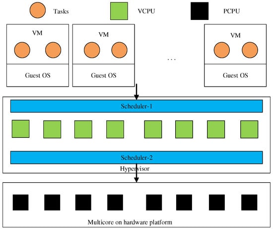
Figure 4.
Illustration of Hierarchical scheduling.
5.2. Schedule Tasks to VCPUs
Note that task scheduling is on the virtualization platform. Only the scheduling of a task is considered. Please note that the virtualization environment can only be accessed by its corresponding DAG task. Therefore, when a DAG task is dispatched on its virtual platform Π, there is no interference from other tasks, and the scheduling of every DAG is independent of other tasks [25]. The goal is to construct a virtualization platform π, on which the deadline of k can be arranged by the Scheduler-1 and guaranteed.
5.3. Schedule VCPUs to PCPUs
Note that the problem of scheduling whole VCPUs together on PCPUs Is similar to task scheduling on the virtualization environment. This problem consists of two issues: how to provide specific services required by virtualization environment on PCPUs, and whether these virtual platforms can be successfully scheduled on PCPUs.
5.4. VCPUs in Hypervisor
The architecture of parallel hierarchical scheduling is described in detail. Every task is a DAG, and these tasks cannot directly use processor resources. Instead, processor resources are used in a shared way through middleware. We define middleware as VCPUs. Figure 5 shows the complete architecture of our platform, which is layered. It will implement our approach on avionic system developed based on a hypervisor. Below, it will introduce the implementation of the two scheduling components and the runtime performance in detail. The first problem is how to allocate processor resources to VCPUs. The second is how OpenMP threads use VCPUs. Because the OpenMP thread and system thread are in a one-to-one relationship, using the OpenMP thread instead of the system thread.
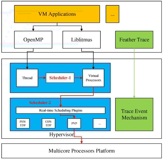
Figure 5.
The architecture of virtualization platform.
6. Results
6.1. Evaluations
This experiment verified the capacity proportional to the number of processors. For every configuration, 1000 tests were conducted on the comparison method. Every experiment casually generates a DAG task. The standardized worst-case maximum CT is used as an index. Figure 6 shows the worst-case maximum CT of the existing method and the proposed method under the different numeral of processors on the DAG generated at p = 8. When m ≤ 4, rta-cpf provides similar results to the classical bound, that is, most of its results are the upper bound of the classical bound. This is because the parallelism of DAG is limited when the numeral of cores is small, so every NC-joint has a long worst-case CT (in Formula (3)). This leads to a lower limit (a higher limit) for every supplier, so the worst-case maximum CT is longer. With the further increase of m, rta-cpf becomes effective (m = 6), and in the case of m = 7.8, it exceeds the classical limit by 15.7% and 16.2% (and as high as 31.7% and 32.2%) on average. In this case, more workloads can be executed in parallel with the CP, that is, the increase of and the decrease of . Therefore, rta-cpf leads to stricter results by explicitly considering this workload, thus safely reducing the interference on the CP. Similar results were obtained in the comparison between rta-cpf-eo and He2019, in which rta-cpf-eo provided a shorter worst-case CT approximation when m ≥ 4, for example, it was as high as 11.1% and 12.0% when m = 7 and m = 8, respectively. We note that the execution order of joints in the two methods will also affect the limit of analyzing the worst case. We compare the scheduling and analysis methods respectively. In short, when m = 7, rta-cpf provides similar results to it, and is superior to it when m = 8. The result shows the usefulness of the proposed method.
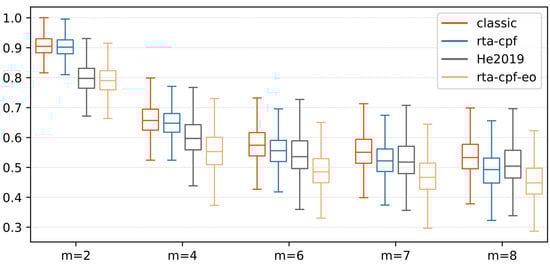
Figure 6.
WC CT of DAG using different numeral of processors.
6.1.1. Sensitivity of DAG Priorities
From some results, it is not easy to understand how the DAG attribute affects the WC maximum CT. To adapt to this situation, this experiment shows how the evaluated analysis is sensitive to some DAG features. That is, by controlling the parameters of Dag and evaluating the maximum CT in the normalized value, we can see how much the performance of the analysis has changed. Otherwise, this will not be distinguished by the WC maximum CT or schedulability analysis. Specifically, we consider the following parameters in this experiment: (i) DAG parallelism (the maximum possible width when generating a randomized DAG), , and (ii) the ratio of DAG CP to total workload %L, where %L = L/C × 100%.
Figure 7 evaluates the influence of CP length on the usefulness of the proposed method, m = 2. The CP varies from 60% to 90% of the total workload of the generated DAG. In this experiment, compared with the existing methods, the proposed analysis shows the most remarkable performance. For the proposed method, due to the change in the internal structure of the generated DAG (for example, L = 0.6), the WC maximum CT of rta-cpf varies with a small amount of %L. However, with the further increase of %L, rta-cpf provides a constant CT because whole non-critical workloads can be executed in parallel with the CP. In this case, the maximum CT is directly equal to the length of the CP. Similar results were obtained for rta-cpf-eo, which provided a constant CT (the length of the CP) under whole experimental settings. Note that, with the further increase of %L, it is completely dominated by rta-cpf. Sensitivity of CP ratio (m = 4, p = 8) in Figure 8.
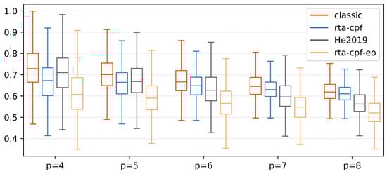
Figure 7.
Sensitivity of parallelism parameter (m = 4).
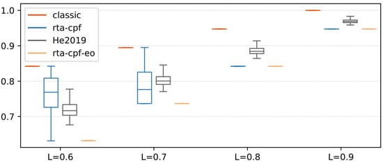
Figure 8.
Sensitivity of CP ratio (m = 4, p = 8).
The method is superior to the classical method and the latest technology in general. In short, we observe that whole the tested parameters have an influence on the function of the proposed method. For rta-cpf, it is sensitive to the relationship between and , in which low or high shows the usefulness of this method. These two factors have a direct impact on the CT of whole NC-joints. %L will also significantly affect the performance of rta-cpf. In rta-cpf, a longer CP usually leads to a more accurate approximation of the maximum CT. Similar to rta-cpf-eo, rta-cpf shows better performance with the increase of% L. Hence, due to its explicit execution sequence, rta-cpf-eo shows stronger performance than rta-cpf, and is not affected by parameter q.
6.1.2. Usefulness of The Proposed Schedulability
The proposed algorithm is compared with the advanced joint-level priority allocation method (namely He2019). In short, it is proved that the WC achieves maximum CT considering priority allocation. The goal is to prove the WC He2019 of improvement, grouped by the numeral of processors m, p = 8, “?” means beat the market. Scenarios are realized through priority allocation. Overall, 1000 random task sets will be generated under every configuration. This evaluation compares two indicators: (i) time suggested rta-cpf-eo is more than the comparison algorithm, (ii) the latency of standardized CT in the improvement cases.
Figure 9 shows the extended comparison between the proposed ranking algorithm and the algorithm in He2019 in the case of different numerals of processors. The frequency denotes the number of cases where the proposed timetable is red or blue. The WC maximum CT analysis for explicit orders is applicable to both orders, so the performance difference comes from the order strategy. From the results, the proposed algorithm is generally superior to it at higher frequencies, especially in the case of a small numeral of cores, for example, in the case of m = 2 near the frequency of 600. With the increase of m, the frequency difference of the method gradually decreases, and it becomes difficult to distinguish when m = 8. In these cases, most joints can execute in parallel, so the influence of different sequences on the final maximum CT becomes less significant.
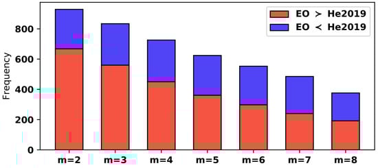
Figure 9.
Compare priority sorting with sorting in He2019.
Table 1 compares the advantages of the two algorithms in detail, expressed as a percentage. For EO > He2019 (that is, the proposed schedule is better than it), the average optimization was observed (in terms of the WC maximum CT) is higher than 5.42% (as high as 7.88%) in all cases. In the case of EO < He2019, the optimization is always lower than that of EO > He2019.

Table 1.
Advantage: percentage of improvement in joint ordering policy.
Table 2 shows the number of advantageous cases and the scientific significance of improvement, He2019 > EO, He2019 < EO. The values in Table 2 are category values to report its importance. Namely, the importance determines if any difference is more than random, and the size of the difference. The data column illustrates the number of times that an algorithm has a lower CT than another. As far as all of the circumstances are concerned, the algorithm is superior to the most advanced algorithm. This order of magnitude further proves the advantages of our algorithm. For example, when m = 4, when EO is superior to He2019, the effect size is medium, but when He2019 is superior to EO, the effect size is small; For m = 8, even if data have similar values, the effect size is small and can be ignored.
Table 2.
The joint-level priority allocation realized in (α, β).
Similarly, by applying the same ranking to the two methods, we compared our analysis with that in He2019, and found consistent results. Therefore, we conclude that the proposed scheduling and analysis is effective and superior to the most advanced technology in general.
6.2. Synthetic Workload
For every DAG task, the number of vertices is casually selected in [50, 250]. The WCET of every vertex is casually selected in [50, 100]. For every possible edge, take a random value in [0, 1], and only add the edge to the graph when the generated value is less than the predefined threshold . Generally, the larger , the more ordered the tasks (namely the longer the CP of DAG). In Figure 10. Comparison of acceptance rates of different dimensions under the comprehensive workload [26].
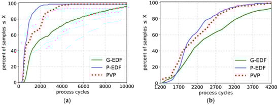
Figure 10.
Comparison of three schedulers; (a) scheduling overhead, (b) context-switch overhead.
Deadline and Period: Periods are generated in an integer power of 2. We find the minimum value A so that , and casually set to one of 2c, 2c + 1 or 2c + 2. When the period of the task is 2c, 2c +1 or 2c +2, the ratio of the task is in the range of [1, 1/2], [1/2, 1/4] or [1/4, 1/8] respectively. The relative cut-off time is uniformly selected from the range .
Figure 11a compares the acceptance rates of task sets with different Standardized utilization rates, where q is 0.1 and is casually generated in the range of [1/8, 1]. Standardized utilization represents the X-axis, and acceptance rates according to the standardized utilization under different processor numerals. It can be observed that SF-XU and H-YANG are superior to G-MEL. This is because SF-XU and H-YANG’s analysis techniques are both carried out under the framework of federal scheduling, eliminating the interference between tasks, while G-MEL is based on RTA, which is much more pessimistic due to the interference between tasks. In short, the performance of H-YANG is better than that of SF-XU because it provides a more efficient resource-sharing solution. Figure 11b compares the acceptance rates of task sets with different intensities. Figure 11b follows the same setup as that of Figure 11a, but generates task cycles at different ratios between . As the x-axis value increases, the tension decreases. The standardized utilization rate of every task is casually selected from [0.1, 1]. Interestingly, with the increase of tension, the gap between these three tests is increasing. It is because, with the increase of the circle in CP length, the problem of resource waste of SF-XU becomes more and more serious, and H-YANG alleviates this problem to some extent.
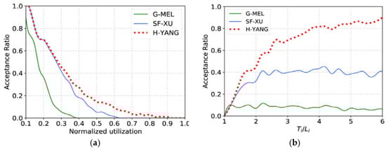
Figure 11.
Comparison of different synthetic workload; (a) Standardized utilization, (b) Tensity.
7. Conclusions
A parallel hierarchical scheduling framework based on DAG tasks with limited deadlines is proposed in this article. Under this framework, the kinds of tasks are not distinguished, and a rule-based scheduling method is proposed which maximizes node parallelism to improve the schedulability of single DAG tasks. Based on the rules, a response-time analysis is developed that provides tighter bounds than existing analysis for (1) any scheduling method that prioritizes the critical path, and (2) scheduling methods with explicit execution order known a priori. We demonstrate that the proposed scheduling and analyzing methods outperform existing techniques. The scheduling framework has been implemented on avionic real-time systems platform, and through experiments, we know that the extra overhead brought by the method proposed in this chapter is acceptable. Finally, a simulation experiment is constructed to verify the adjustability of the framework. The experimental results demonstrate that the strategy proposed have better performance in the article.
Based on the research conclusion of this article, there are still many directions worthy of further analysis in the future. First, we can consider scheduling multi-DAG task models on a given virtual computing platform according to different resource interfaces. Moreover, sharing resource models among DAG tasks is also an important direction for us to consider. Energy-sensitive scheduling algorithm for the DAG task model is also worthy of attention.
Author Contributions
Conceptualization, H.Y. and S.Z. (Shuang Zhang); methodology, H.Y. and S.Z. (Shuai Zhao); software, H.Y. and S.Z. (Shuai Zhao); validation, Y.G., H.Y. and X.S.; formal analysis, Y.G.; investigation, H.Y.; resources, S.Z. (Shuang Zhang); data curation, X.S.; writing—original draft preparation, H.Y.; writing—review and editing, Y.G.; visualization, X.S.; supervision, S.Z. (Shuang Zhang); project administration, S.Z. (Shuang Zhang); funding acquisition, H.Y. All authors have read and agreed to the published version of the manuscript.
Funding
This research was funded by National Key Scientific Research Projects of China, grant numeral MJ-2018-S-34.
Institutional Review Board Statement
Not applicable.
Informed Consent Statement
Not applicable.
Data Availability Statement
Not applicable.
Acknowledgments
The work was supported by the school of computer at Northwestern Polytechnical University, some colleagues in University of York and Xi’an Aeronautical Computing Technique Research Institute.
Conflicts of Interest
The authors declare no conflict of interest.
References
- Alonso, A.; de la Puente, J.; Zamorano, J.; de Miguel, M.; Salazar, E.; Garrido, J. Safety concept for a mixed criticality on-board software system. IFAC PapersOnLine 2015, 48, 240–245. [Google Scholar] [CrossRef]
- Burns, A.; Davis, R. A survey of research into mixed criticality systems. ACM Calc. Surv. 2017, 50, 1–37. [Google Scholar] [CrossRef]
- Burns, A.; Davis, R. Mixed Criticality Systems: A Review; Technical Report MCC-1(L); Department of Calculater Science, University of York: York, UK, 2019; p. 6. Available online: http://www-users.cs.york.ac.uk/burns/review.pdf (accessed on 10 March 2019).
- LynxSecure. Available online: https://www.lynx.com/products/lynxsecure-separation-kernel-hypervisor (accessed on 14 January 2021).
- QNX Adaptive Partitioning Thread Scheduler. Available online: https://www.qnx.com/developers/docs/7.0.0/index.html#com.qnx.doc.neutrino.sys_arch/topic/adaptive.html (accessed on 14 January 2021).
- QNX Hypervisor. Available online: https://blackberry.qnx.com/en/software-solutions/embedded-software/industrial/qnx-hypervisor (accessed on 14 January 2021).
- QNX Platform for Digital Cockpits. Available online: https://blackberry.qnx.com/content/dam/qnx/products/bts-digital-cockpits-product-brief.pdf (accessed on 14 January 2021).
- Wind River Helix Virtualization Platform. Available online: https://www.windriver.com/products/helix-platform/ (accessed on 18 June 2021).
- Wind River VxWorks 653 Platform. Available online: https://www.windriver.com/products/vxworks/certification-profiles/#vxworks_653 (accessed on 18 June 2019).
- Baruah, S. The Federated Scheduling of Systems of Conditional Sporadic DAG Tasks. In Proceedings of the 12th International Conference on Embedded Software, Amsterdam, The Netherlands, 4–9 October 2015; pp. 1–10. [Google Scholar]
- Li, J.; Chen, J.; Agrawal, K.; Lu, C.; Gill, C.; Saifullah, A. Analysis of Federated and Global Scheduling for Parallel Real-Time Tasks. In Proceedings of the 26th Euromicro Conference on Real-Time Systems, Madrid, Spain, 8–11 July 2014; pp. 85–96. [Google Scholar]
- Xu, J.; Nan, G.; Xiang, L.; Wang, Y. Semi-Federated Scheduling of Parallel Real-Time Tasks on Multiprocessors. In Proceedings of the 2017 IEEE Real-Time Systems Symposium (RTSS), Paris, France, 5–8 December 2017; pp. 80–91. [Google Scholar]
- He, Q.; Jiang, X.; Guan, N.; Guo, Z. Intra-task priority assignment in real-time scheduling of DAG tasks on multi-cores. IEEE Trans. Parallel Distrib. Syst. 2019, 30, 2283–2295. [Google Scholar] [CrossRef]
- Melani, A.; Bertogna, M.; Bonifaci, V.; Marchetti-Spaccamela, A.; Buttazzo, G.C. Response-Time Analysis of Conditional DAG Tasks in Multiprocessor Systems. In Proceedings of the Euromicro Conference on Real-Time Systems, Lund, Sweden, 8–10 July 2015; pp. 211–221. [Google Scholar]
- Graham, R.L. Bounds on multiprocessing timing anomalies. J. Appl. Math. 1969, 17, 416–429. [Google Scholar] [CrossRef]
- Fonseca, J.; Nelissen, G.; Nélis, V. Improved Response Time Analysis of Sporadic DAG Tasks for Global FP Scheduling. In Proceedings of the International Conference on Real-Time Networks and Systems, Grenoble, France, 4–6 October 2017; pp. 28–37. [Google Scholar]
- Chen, P.; Liu, W.; Jiang, X.; He, Q.; Guan, N. Timing-anomaly free dynamic scheduling of conditional DAG tasks on multi-core systems. ACM Trans. Embed. Comput. Syst. 2019, 18, 1–19. [Google Scholar] [CrossRef]
- Chang, S.; Zhao, X.; Liu, Z.; Deng, Q. Real-time scheduling and analysis of parallel tasks on heterogeneous multi-cores. J. Syst. Archit. 2020, 105, 101704. [Google Scholar] [CrossRef]
- Guan, F.; Qiao, J.; Han, Y. DAG-fluid: A real-time scheduling algorithm for DAGs. IEEE Trans. Calc. 2020, 70, 471–482. [Google Scholar] [CrossRef]
- Topcuoglu, H.; Hariri, S.; Wu, M.-y. Performance-effective and low-complexity task scheduling for heterogeneous computing. IEEE Trans. Parallel Distrib. Syst. 2002, 13, 260–274. [Google Scholar] [CrossRef]
- Lin, H.; Li, M.-F.; Jia, C.-F.; Liu, J.-N.; An, H. Degree-of-joint task scheduling of fine-grained parallel programs on heterogeneous systems. J. Calc. Sci. Technol. 2019, 34, 1096–1108. [Google Scholar]
- Zhao, S.; Dai, X.; Bate, I.; Burns, A.; Chang, W. DAG Scheduling and Analysis on Multiprocessor Systems: Exploitation of Parallelism and Dependency. In Proceedings of the 2020 IEEE Real-Time Systems Symposium (RTSS), Houston, TX, USA, 1–4 December 2020; pp. 28–40. [Google Scholar]
- Zhao, S.; Dai, X.; Bate, I. DAG Scheduling and Analysis on Multi-Core Systems by Modelling Parallelism and Dependency. IEEE Trans. Parallel Distrib. Syst. 2022, 33, 231–245. [Google Scholar] [CrossRef]
- Jiang, X.; Guan, N.; Long, X.; Wan, H. Decomposition-based Real-Time Scheduling of Parallel Tasks on Multi-cores Platforms. IEEE Trans. Calc. Aided Des. Integr. Circuits Syst. 2019, 39, 183–198. [Google Scholar]
- Yang, T.; Deng, Q.; Sun, L. Building real-time parallel task systems on multi-cores: A hierarchical scheduling approach. J. Syst. Archit. 2019, 92, 1–11. [Google Scholar] [CrossRef]
- Saifullah, A.; Ferry, D.; Li, J.; Agrawal, K.; Lu, C.; Gill, C. Parallel real-time scheduling of dags. Parallel Distrib. Syst. IEEE Trans. 2014, 25, 3242–3252. [Google Scholar] [CrossRef]


Disclaimer/Publisher’s Note: The statements, opinions and data contained in all publications are solely those of the individual author(s) and contributor(s) and not of MDPI and/or the editor(s). MDPI and/or the editor(s) disclaim responsibility for any injury to people or property resulting from any ideas, methods, instructions or products referred to in the content. |
© 2023 by the authors. Licensee MDPI, Basel, Switzerland. This article is an open access article distributed under the terms and conditions of the Creative Commons Attribution (CC BY) license (https://creativecommons.org/licenses/by/4.0/).