Abstract
Road tunnels are equipped with various safety installations that enable the tunnel’s autonomous response to fire in order to ensure conditions suitable for safe self-rescue and evacuation. A key role in this effort is played by the monitoring of the longitudinal airflow velocity and its regulation. This study contributes to validation of the Fire Dynamics Simulator (FDS 6) capabilities to model tunnel airflow generated by emergency ventilation. A previous study, in which an FDS 6 model of a real 900 m long motorway tunnel was developed and validated by a full-scale ventilation test, pointed to the relatively high inaccuracies of the average steady-state airflow velocity generated by ventilation measured by tunnel anemometers (13%, 17% and 14% for three ventilation modes). In this paper, it is shown that the application of a modified evaluation procedure and improving the representation of tunnel anemometers leads to the significant improvement of simulation results with inaccuracies of 5%, 1% and 3% for the considered ventilation modes. The observed inaccuracies are even comparable to the measurement accuracy of the tunnel anemometers. A further extension of the modeling of the steady-state airflow velocity generated by emergency ventilation measured by the used anemometers is also described.
1. Introduction
Fires in tunnels can cause considerable material and environmental damage and loss of life and health of tunnel users. Road tunnels belong to such capital-intensive construction projects, which often contribute to solving acute traffic problems in the region, protecting the environment and reducing the number of road accidents. They are considered as ecological structures protecting nature and original habitats, as they do not negatively affect the migration of animals. Tunnels are often part of supra-regional or transnational transport corridors and national critical infrastructures. A fire in a tunnel is considered to be one of the most destructive events that can cause significant secondary damage with a transnational impact due to a long-term interruption, or operation disruptions during tunnel closures. Therefore, special attention is paid to fire prevention, safe operation and resilience of the tunnel, as well as to readiness for firefighting and rescue work. The tunnel is considered as an intelligent structure that is equipped with many safety installations, such as traffic control system, emergency ventilation, camera monitoring system, emergency lighting, emergency power supply, measurement of physical quantities, etc. These installations are used by the central control system (CCS) for autonomous fire detection, ensuring conditions inside the tunnel suitable for safe self-rescue and evacuation, to prevent entry into the affected tunnel tube and to provide the necessary information for the escape of people until the arrival of firefighters and rescuers. This CCS effort is supported by tunnel control operators who continuously monitor the situation inside the tunnel and can also participate in fire detection and localization using fire detection and camera monitoring systems. One of the key tasks of the CCS in the event of a fire is to monitor the airflow velocity inside the tunnel and to regulate it using emergency ventilation to create and to maintain conditions suitable for smoke stratification in the upper part of the tunnel. The proper functioning of all tunnel safety systems and the readiness of tunnel control operators, firefighters and rescuers is critical for mitigating damage and preventing the loss of lives. For various possible fire scenarios, for each tunnel, there are pre-prepared and tested automatic responses of the tunnel to fire, which include various emergency ventilation operation strategies. These ventilation tests are conducted in the tunnel even before it is put into operation.
Computer simulation of fires is, at present, considered to be an effective means of preventing fires, increasing preparedness to deal with them and mitigating their consequences. Considerable efforts towards more accurate and reliable mathematical and physical fire models have led to the development of advanced simulation systems for modeling fires in a variety of important environments. Experimental investigation of fire behavior outside the laboratory is expensive and allows only a limited number of fire scenarios to be investigated. Such an experiment often leads to the destruction of the tested structure. The goal is therefore to develop such a software environment that will enable to reliably simulate the behavior of a real fire in a given structure using 3D visualization. Such a simulation makes it possible to flexibly change the parameters of the fire scenario according to the user’s requirements at present, and to test different extinguishing strategies and their effectiveness.
Computational Fluid Dynamics (CFD) techniques are at present often used to design and test ventilation systems and to simulate fire and smoke. The two most popular software tools are Fire Dynamics Simulator (FDS) and ANSYS Fluent. FDS is primarily used to simulate fire development [1,2] and ANSYS Fluent is a multi-purpose package that can be used for any fluid and heat flow problem [3]. However, designing a simulation using both systems requires making certain design decisions, taking into account all relevant approximations and simplifications of the models and justifying them thoroughly [4].
FDS [5] is a CFD solver widely used for various applications, not only for solving practical problems in fire protection technology, but also for studying basic fire dynamics. It is an open-source code developed at NIST (National Institute of Standards and Technology, USA), which simulates basic physical and chemical processes related to fire, such as combustion, pyrolysis, thermal radiation, air circulation dynamics, airflows induced by fire, turbulence, fire suppression, etc. Some of the major features of the FDS code are the low-Mach large-eddy simulation, explicit second-order kinetic-energy-conserving numerics, Deardorff eddy viscosity, gray gas radiation, etc. These features have been widely used and validated for over two decades. FDS enables various types of 2D and 3D visualizations of fire courses and parameters. The complex dynamics of fire processes requires detailed resolution of the numerical mesh and a short time step to achieve sufficient calculation accuracy, which is demanding on computer performance and memory. FDS enables the simulation to be conducted in parallel on various platforms of high-performance computers to date.
There is extensive literature describing the various aspects of modeling fire and toxic smoke spread using FDS, modeling the course and effects of a fire and also modeling evacuation during a fire. Most researchers use laboratory-obtained data from small-scale models to validate simulations. Although there are a high number of practical applications in which FDS is used, there are not many papers in the literature dealing with the validation of tunnel fire simulation using data from large-scale experiments [6,7,8,9,10], or such studies remain unpublished. The first validation study related to the FDS simulation of ventilation in a tunnel used a full-scale fire experiment conducted as part of the Massachusetts Highway Department Memorial Tunnel Fire Ventilation Test Program [6]. The test consisted of a single-point supply of fresh air through a 28 m2 opening in a 135 m tunnel. In [7], a coupled hybrid (1D/3D-CFD) modeling methodology using the FDS 6 (version 6.7.5) was validated by full-scale fire tests in the 1600 m long Runehamar tunnel. For 6, 66 and 119 MW fires, temperature profiles, centerline velocity, backlayering lengths and maximum temperatures upstream and downstream from the fire source were investigated. The study [8] examined three evacuation scenarios after a 20 MW fire accident in a 1500 m long railway tunnel with longitudinal ventilation and different ventilation activation times. The fire characteristics simulated by FDS were compared with empirical formulae based on small- and full-scale fire experiments. To investigate the effectiveness of water spray in blocking smoke and heat in a short underground belt transport tunnel in a mine with mechanical ventilation and a water curtain system, a full-scale fire test was conducted measuring selected fire characteristics [9]. FDS (version 6.0.1) was then used to simulate smoke-spread characteristics, temperature distribution, visibility profiles and CO distribution. In [10], a series of full-scale experiments with 1.35, 3 and 3.8 MW fires conducted in a short metro tunnel with mechanical ventilation system was described and then simulated by FDS (version 5.5). The smoke temperature and decay rate of the temperature distribution under the tunnel ceiling were investigated.
There are not many papers related to the validation of an airflow generated by emergency ventilation in a real tunnel (even without fire). However, the accurate reproduction of tunnel airflow is a key issue in modeling the operation of the tunnel ventilation system at any mode or fire development and smoke propagation in the event of fire [4,11]. To increase the confidence of practitioners and researchers in the ability of FDS to capture tunnel airflow, the average airflow velocity and velocity profile in the Dartford Tunnel (UK) were simulated using FDS 6 and then compared with in situ measurements [12]. The tunnel is 1430 m long with a circular cross-section with a diameter of 8.5 m. Although it was modeled as a tunnel with a square cross-section, the results correlate well with the measurements. This research demonstrates the ability of FDS to simulate jet fans and the airflow they create. In [13,14], the airflow generated by jet fans with a relatively small diameter, which are popular in car park ventilation systems, was investigated. The suitability of different implementations of the turbulence model in the FDS 6 system for simulating such airflow was also discussed. The research confirmed the FDS 6’s ability to simulate airflow velocities generated by jet fans in larger enclosures. An important issue related to the modeling of airflow in the tunnel is the effect of reducing the thrust efficiency of the jet fan. This effect was experimentally studied in [15,16]. According to [17], such losses due to momentum transfer and high shear stress of the wall can reach up to 20–30%. Installing the jet fans close to walls causes increased wall shear stress around the jet. In [17], the results of two full-scale measurements of different jet fan installations were investigated in order to analyze the efficiency of the installation. These measurements were used to design and validate a numerical model.
In [18], an FDS 6 model of the 898 m long Polana tunnel (Slovakia) was developed and its ability to simulate airflow generated by emergency ventilation was tested. The model was validated using a full-scale in situ ventilation test. A method of adjusting the parameters of the tunnel walls was proposed, reflecting the effect of the reduction in the thrust efficiency of the jet fans and the FDS limitations related to the resolution and type of the numerical mesh. One of the three tested ventilation operation modes was used to set up the model, and then the data from the entire ventilation test were used to validate the model with respect to time-averaged steady-state airflow velocities. A comparison with the experimental data confirmed the very good accuracy of the simulation results of the time-averaged velocity measured by a grid of anemometers located in the tunnel cross-section, but pointed to a relatively lower accuracy of the simulation for the tunnel anemometers.
In this paper, we analyze the simulation results presented in [18], propose an improved representation of tunnel anemometers and contribute to a better validation of the model. A substantial improvement in the modeling accuracy of the airflow velocity determined by tunnel anemometers is demonstrated. The data from the ventilation test are used to validate the improved model with respect to the average velocity and the time-averaged velocity of the steady-state ventilation-generated airflow measured by grid and tunnel anemometers.
2. Materials and Methods
2.1. Ventilation Tests in the Polana Tunnel
The Polana tunnel [18,19,20] is a single-tube, bi-directional, 898 m long tunnel with a horse-shoe-shaped cross-section that has been in operation since 2017 (Figure 1). It is located near the D3 motorway in the north of Slovakia near the border with Poland. The D3 motorway is part of the European multimodal transport corridor VI, ensuring a fast connection of Northern and Eastern Europe. Direct and indirect losses caused by a potential fire in the Polana tunnel could therefore exceed the national level. The tunnel is 6.8 m high and 10 m wide with a cross-section area of 60.3 m2, and an 8 m wide carriageway. Two emergency lay-bys are located at a distance of 373 and 635.6 m from the left (western) portal of the tunnel, one for each direction. At the lay-bys level, the tunnel is 7.5 m high and 12.8 m wide. The lay-by niches are 50 m long. Both lay-bys are constructed as one-sided and, with their asymmetric geometry, significantly affect the airflow and smoke stratification inside the lay-bys and in their vicinity (see, e.g., studies [21,22]). The tunnel has a 2% ascending slope. At the end of each lay-by there is a prism-shaped emergency bumper, which is shown in Figure 1 (top, left).
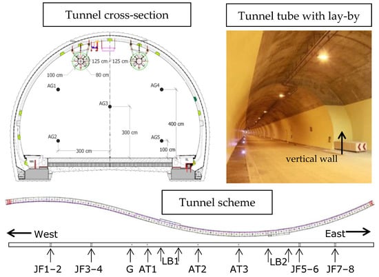
Figure 1.
Polana tunnel: tunnel cross-section with locations of grid anemometers AG1–5 and the jet fans (top, left); tunnel tube with emergency lay-by and the lay-by’s vertical wall acting as an obstruction against the airflow highlighted by the arrow (top, right); and tunnel scheme with the determined west–east orientation, locations of jet fans JF1–8, grid G consisting of anemometers AG1–5, lay-bys LB1–2 and tunnel anemometers AT1–3 in the tunnel (bottom).
The tunnel is equipped with various safety installations, such as a linear heat detector, measurement of physical quantities, emergency ventilation, smoke detectors, emergency broadcasting, lighting and signaling, camera surveillance, etc. The longitudinal ventilation consists of 4 pairs of axial jet fans located at distances of 101, 201, 716 and 801 m from the left portal of the tunnel. They are installed at a height of 5.1 m above the road. Each individual jet fan has a fan wheel diameter of 0.8 m, a shroud length of 3.7 m, a maximum volume flow rate of 19 m3/s, an airflow velocity at the fan outlet of 38.5 m/s and a thrust in the main direction of 850 N. The aim of the ventilation in case of a fire is to create and maintain tenable conditions for tunnel users and to ensure their safe evacuation, i.e., by regulating the longitudinal airflow and stabilizing the longitudinal airflow velocity in the tunnel to a target value. In the Polana tunnel, the aim is to reach such conditions within 120 s by a step-less continuous airflow regulation using axial jet fans, which are controlled by frequency converters [23]. The measurement of airflow velocity installed in the Polana tunnel consists of 3 ultrasonic anemometers with a measurement accuracy of 0.1 m/s. They are located at distances of 340, 465 and 565 m from the left portal of the tunnel. These devices work on the basis of measuring the transit delay of ultrasonic pulses. Each anemometer contains transmitter/receiver units for transmitting and receiving ultrasonic pulses, mounted on both sides of the tunnel at a certain angle to the direction of the airflow.
In 2017, a series of ventilation tests was conducted in the Polana tunnel. The objective of one of these tests was to measure the longitudinal airflow velocity in the empty tunnel using the grid of 5 anemometers (AG1–5) located 300 m from the left portal of the tunnel [23] (Figure 1). Three ventilation scenarios were tested, corresponding to three modes of ventilation operation described in Table 1 and Figure 2. The aim of the test was to create a relatively stable airflow in the tunnel at the given ventilation power, to maintain it for a certain period of time, and thus to enable the measurement of the longitudinal velocity of the steady flow generated by the jet fans. The average airflow velocity was determined as the average of the velocities measured by the grid anemometers AG1–5 (with a measurement accuracy of 0.3 m/s) and as the average of the velocities measured by the tunnel anemometers AT1–3 (with a measurement accuracy of 0.1 m/s) (Figure 3). The data recording frequency was 10 s.

Table 1.
Description of 3 ventilation operation modes tested during the ventilation test.
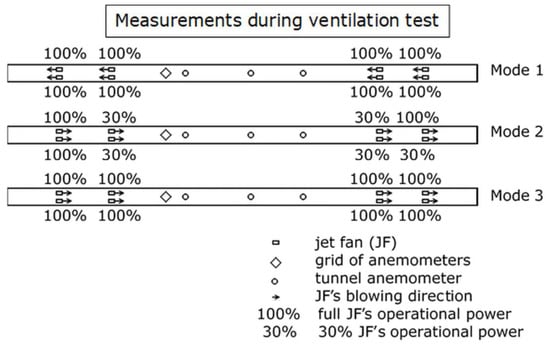
Figure 2.
Scheme of measurements conducted during the tested ventilation scenarios (modes 1–3): direction and operational power of individual jet fans are highlighted by arrows and percentage of the full operation power of individual jet fan; individual jet fans, location of grid of anemometers and tunnel anemometers are illustrated schematically.
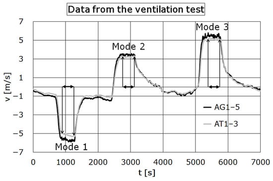
Figure 3.
Average airflow velocity v [m/s] measured by the grid anemometers AG1–5 (black curve) and the tunnel anemometers AT1–3 (gray curve). The 6 min time intervals, where the airflows were considered stabilized, are highlighted by arrows.
As it can be seen from the velocity values shown in Figure 3, the Mode 1 scenario represents a westward flow corresponding to negative velocity values, while the other two scenarios, modes 2 and 3, represent an eastward flow corresponding to positive velocity values. The 6 min time intervals, where airflow velocities were considered to be stabilized during the three ventilation operation modes, are highlighted by arrows in the figure.
At the time of the test, meteorological stations had not yet been installed in the vicinity of the tunnel portals; therefore, the data on wind speed and direction were not available. However, local measurements indicated a temperature inside the tunnel of 6.0 °C and an outside temperature of 5.5 °C.
2.2. Computer Modeling of the Ventilation Test
In this section, we follow the procedure for creating the FDS model of the Polana tunnel proposed in [18] in order to create an improved FDS model that better estimates the airflow velocity generated by the ventilation. Since the simulation results obtained in this paper need to be compared with those reported in [18], we used the same simulator version (FDS, version 6.5.2; MPI, version 3.0; MPI library, version Intel® MPI Library 5.1.3) as was used there.
The geometrical representation of the Polana tunnel and its equipment (tunnel tube, emergency lay-bys, jet fans, vertical traffic signs, emergency bumpers in the lay-bys) for the FDS environment was modeled and adjusted with regard to the selected computational mesh resolution. All the dimensions and locations as well as the jet fan’s performance are in accordance with the Polana tunnel. In the final simulation, a 30 cm computational mesh resolution was used; therefore, the following description of the simulation parameters corresponds to this resolution.
The calculation was parallelized using the MPI (Message Passing Interface) model due to its high computational efficiency. The discussion on the model’s sensitivity to the resolution of the computational mesh and the simulation parallelization is included in Appendix A. According to this analysis, the decomposition of the computational domain into 12 meshes of the same size and mesh resolution, and the computational mesh resolution of 30 cm seems to be optimal; therefore, these settings were used in this study. The same settings were also used for the final simulations in [18]. The computational domain had dimensions of 900 m × 18 m × 8.1 m and consisted of 3000 × 60 × 27 = 4,860,000 mesh cells. The mesh cell number of each particular computational mesh was 405,000.
The axial jet fans were modeled by the HVAC subsystem of FDS 6, which is used for modeling HVAC (Heating, Ventilation and Air Conditioning) systems [5]. Each jet fan is represented by a pair of 0.9 m × 0.6 m rectangular vents with a prescribed normal velocity, using the HVAC to model the inlet and outlet of the jet fan. The modeled jet fan shroud was represented by 4 rectangular OBSTRUCTIONs of 1 mesh-cell thickness surrounding the jet fan. The length of the jet fan shroud was set to 3.9 m due to the selected mesh resolution. The maximum volume flow in the HVAC settings was slightly adjusted [18] to achieve the same pressure rise in the tunnel [17] and to transfer the same momentum to the computational domain. Therefore, in the HVAC settings, a volume flow rate of 19.75 m3/s was used to conserve Avj2, where A is the area of the modeled (0.54 m2) and actual (0.5 m2) jet fan, and vj is the jet velocity at the fan outlet. The time dependence of the volume flow rate of the jet fans in operation was set by the RAMP corresponding to their performance during the ventilation test. The gradual jet fan onset was modeled by a 115 s interval of linear increase in the power of jet fan included in the RAMP directing the operation of the jet fan. The location of the jet fans and all the anemometers (5 grid anemometers and 3 ultrasonic tunnel anemometers) in the tunnel were adjusted to be consistent with their location during the ventilation test. The measurement of the airflow velocity by a particular tunnel anemometer was modeled as an average velocity measured in a one-cell-thick volume located at a height of 5.2 m between the locations on both sides of the tunnel where the anemometer transmitter/receiver units were mounted. The grid anemometers were modeled as point devices for measuring the airflow velocity.
The values of 6.0 °C and 5.5 °C were used for the temperature inside the tunnel and for the outside temperature. The wind and pressure conditions at the tunnel portals were represented by the dynamic pressure at the tunnel portals, which was estimated to approximate the correct values of the airflow velocity at the time when the jet fans were turned off (see Figure 3).
Velocity boundary conditions at rough solid surfaces were specified in FDS using the log law [24], setting the ROUGHNESS parameter (absolute roughness) of the solid surface. However, the limitation of FDS to a rectilinear computational mesh of a certain resolution did not allow a direct representation of all the tunnel geometry details, especially those with dimensions too small in comparison with the mesh resolution (e.g., cables, measuring devices, cameras and lights and their supporting structures, niches) and curved surfaces. To represent the tunnel airflow deceleration caused by the effect of geometric details having an impact on tunnel airflow, but being too small or not possible to be explicitly modeled due to FDS limitations, a tunnel wall roughness adjustment method was proposed and validated for the Polana tunnel in [18]. The data from the first ventilation test (Mode 1) were used to set up the model, and then the data from the entire ventilation test (modes 1–3) were used for the model validate. In accordance with this procedure, we set the material of the tunnel walls and the road to CONCRETE1 and CONCRETE2 and the ROUGHNESS to values of 0.070 and 0.003 m. The simulation of the whole ventilation test (modes 1–3) had a duration of 7180 s (Figure 3). Selected simulation settings are summarized in Table 2.
Table 2.
Main simulation settings.
3. Results and Discussion
The simulation described above was performed on the Intel(R) Core(TM) i7-8700K CPU@3.7 GHz computer (6 cores, 64 GB RAM). In this section, the simulation results are compared with the ones reported in [18], where the results were validated in regard of the time-averaged airflow velocities within selected time intervals where the airflow velocity was considered to be stabilized. In [18], a very good agreement of simulated and experimental results was reported for the velocities measured by the grid anemometers; however, a relatively lower accuracy was observed for velocities measured by the tunnel anemometers. The improved model and validation procedure described in this paper can be characterized as follows:
- More suitable representation of tunnel anemometers in the improved model better corresponds to the actual measurement of airflow velocity in the Polana tunnel (in [18]; the measurement by the tunnel anemometer was represented as a two-point measurement of the airflow velocity on both sides of the tunnel).
- Improved evaluation procedure considers:
- Time intervals, where the airflow is considered to be stabilized, of the same length (in previous evaluation they had various lengths [18]);
- The same number of values is taken into account for all ventilation modes (in [18], different frequencies of the velocity values recording for experimental data and for the simulation were considered);
- Extended evaluation of average velocity values.
The analysis focused on the airflows generated by the three operation modes of ventilation operation (modes 1–3) during which the ventilation relatively soon created a stabilized airflow, the velocity of which was measured by the grid and tunnel anemometers. The average airflow and time-averaged airflow velocities at selected time intervals, where the airflow velocity was considered to be stabilized, were calculated. For the three individual ventilation modes, the 6 min time intervals 900–1260, 2760–3120 and 5390–5750 s were considered. We noted that although the Mode 1 ventilation scenario was used to set up the model’s parameters, in the following section, we include it when evaluating the simulation results as well, due to completeness.
3.1. Modeling Average Airflow Velocity Measured by the Grid Anemometers
In Figure 4, the values of the average airflow velocities in the experiment (represented by the black curve) and simulation (represented by the red curve) are shown. They were calculated as an arithmetic mean of the airflow velocities measured by the grid anemometers (AG1–5) for all the three ventilation modes measured at the considered time intervals by the grid anemometers. Relatively small differences between the experimental and simulation data can be observed. In Figure 5 and Figure 6, absolute and relative differences between the average airflow velocities obtained by the experiment and the simulation are illustrated for all the three ventilation modes. The maximal values of the differences are shown in Table 3. The results indicate that the average velocities measured by the grid anemometers in the simulation differ from the experimental data by values lower (or in exceptional cases by relatively very close values) than the measurement accuracy of the grid anemometers (0.3 m/s). This evaluation indicates a relatively very good accuracy of average airflow velocity modeling using grid anemometers compared to the measurement accuracy of the grid anemometers.
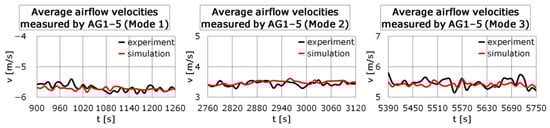
Figure 4.
Average airflow velocities v [m/s] within the considered time intervals measured by the grid anemometers in the experiment (black curve) and simulation (red curve).
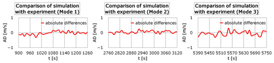
Figure 5.
Absolute differences AD [m/s] between the experimental and simulated averaged airflow velocities determined by the grid anemometers (red curve).
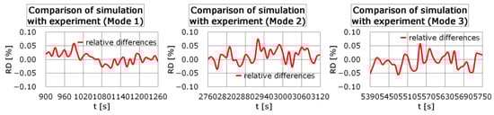
Figure 6.
Relative differences RDs [%] between the experimental and simulated averaged airflow velocities determined by the grid anemometers (red curve).
Table 3.
Maximum and minimum difference AD* [m/s] between the experimental and simulated average airflow velocities measured by the grid anemometers.
3.2. Modeling Time-Averaged Airflow Velocity Measured by the Grid Anemometers
In this section, we followed the evaluation presented in [18] in regard to the values of the time-averaged airflow velocities measured at selected time intervals by the grid anemometers (AG1–5). The comparison of the velocity values calculated by the procedure described here and the one reported in [18] is shown in Table 4, Table 5 and Table 6. The results indicate that the time-averaged airflow velocities obtained by both procedures differ from the experimental data by values significantly lower than the measurement accuracy of grid anemometers (0.3 m/s) for all the ventilation modes. This points to the high accuracy of the airflow velocity modeling by the grid measurement compared to the measurement accuracy of the grid anemometers.
Table 4.
Time-averaged airflow velocity vavg [m/s] determined by the grid anemometers in the experiment (ExpAG) and in both considered simulations (SimAG and [18]).
Table 5.
Absolute difference AD [m/s] between the experimental and simulated time-averaged airflow velocities determined by the grid anemometers.
Table 6.
Relative difference RD [%] between the experimental and simulated time-averaged airflow velocities determined by the grid anemometers.
3.3. Modeling Average Velocity Measured by the Tunnel Anemometers
In Figure 7, the average airflow velocities measured by the tunnel anemometers AT1–3 in the experiment and in both simulations in the considered time intervals are illustrated. The figure indicates that the improved representation of the tunnel anemometers in the simulation (represented by the red color) presents significantly less differences in the simulation results from the experimental data (represented by the black color), while the simulation results reported in [18] (represented by the yellow curve) relatively significantly overestimate the values of the average airflow velocity in Mode 1 and underestimate the values of the average airflow velocity in both the other tested modes of ventilation operation (modes 2–3). In Figure 8 and Figure 9, the absolute and relative differences between the average airflow velocities obtained by both the considered simulations and experimental data are illustrated. In Table 7, the maximum and minimum differences between experimental and simulated average airflow velocities are shown. The curves indicate that the result’s accuracy corresponding to the simulation presented here is much better than the one corresponding to the simulation from [18]. The average airflow velocities measured by the tunnel anemometers in both the simulations differ from the experimental data by values greater than the measurement accuracy of the tunnel anemometers (in the case of Mode 2 in the simulation presented in this paper by slightly higher values). However, the difference in the accuracy of the considered simulations is noticeable (Table 7).
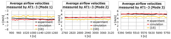
Figure 7.
Average airflow velocities v [m/s] measured by the tunnel anemometers AT1–3 within the considered time intervals in the simulation presented in this paper (red curve), in the experiment (black curve) and in the simulation in [18] (yellow curve).
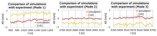
Figure 8.
Absolute differences ADs [m/s] between the experimental and simulated averaged airflow velocities determined by the tunnel anemometers for the simulation presented in this paper (red curve) and the simulation in [18] (yellow curve).
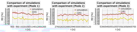
Figure 9.
Relative differences RDs [%] between the experimental and simulated averaged airflow velocities determined by the tunnel anemometers for the simulation presented in this paper (red curve) and the simulation in [18] (yellow curve).
Table 7.
Maximum and minimum differences AD* [m/s] between experimental and simulated average airflow velocities determined by the tunnel anemometers.
3.4. Modeling Average Velocity Measured by the Tunnel Anemometers: Moving Average
When evaluating the simulation results, we to date considered the velocity values measured by tunnel anemometers, which tend to slightly fluctuate, even though in practice it is customary to consider several velocity values when monitoring and evaluating the airflow velocity at a given time. Therefore, in Figure 10, Figure 11 and Figure 12 we present a 5-point moving average of the corresponding velocity values to illustrate the underlying trends of the measured velocity in the experimental data and in both the simulations. In this way, we eliminated to some extent the tendency of the velocity values to fluctuate slightly, similarly to what the tunnel’s CCS does. In Table 8, the maximum and minimum differences between experimental and simulated average airflow velocities determined by moving average are shown. The illustrations confirm the large difference between the results’ accuracies of the simulation presented in this paper and in [18]. Relatively sufficient (although less) accuracy with respect to the measurement accuracy of the tunnel anemometers it can be observed for modes 2 and 3. The accuracy for model 1 is lower, but can still be considered sufficient for practical purposes. However, relatively high inaccuracies in the simulation results presented in [18] are observed. From this analysis, it can be concluded that the improved representation of the tunnel anemometers significantly increased the accuracy of the simulation, and the achieved accuracy appears to be sufficient for the practical use.
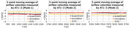
Figure 10.
Five-point moving average of the airflow velocities v [m/s] measured by the tunnel anemometers AT1–3 in the considered time intervals in the simulation presented in this paper (red curve), in the experiment (black curve) and in the simulation in [18] (yellow curve).
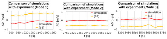
Figure 11.
Absolute differences ADs [m/s] between the experimental and simulated 5-point moving average of the airflow velocities determined by tunnel anemometers for the simulation presented in this paper (red curve) and the simulation in [18] (yellow curve).
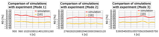
Figure 12.
Relative differences RDs [%] between the experimental and simulated 5-point moving average of the airflow velocities determined by tunnel anemometers for the simulation presented in this paper (red curve) and the simulation in [18] (yellow curve).
Table 8.
Maximum and minimum difference AD* [m/s] between the experimental and simulated average airflow velocities determined by the tunnel anemometers using moving average.
3.5. Modeling Time-Averaged Airflow Velocity Measured by the Tunnel Anemometers
In this section, we again followed the evaluation presented in [18] to illustrate the significant improvement in the accuracy of the results presented here related to the accuracy of measurement of the value of the stable airflow velocity generated by the ventilation.
In Table 9, Table 10 and Table 11, the time-averaged airflow velocities measured by the tunnel anemometers AT1–3 in the considered time intervals in the experiment and in both simulations and their comparison are shown. The tables indicate that the time-averaged velocity obtained based on measurements by tunnel anemometers in the simulation reported in [18] differs from the time-averaged velocity obtained from experimental data from the tunnel anemometers by significantly more than the accuracy value of the grid anemometers (0.3 m/s), which points to the insufficient accuracy of the used representation of the measurement by tunnel anemometers. The results of the simulation presented in this paper indicate a significant increase in the accuracy of modeling the measurement by the tunnel anemometers, while the deviations from experimentally obtained values are less than the accuracy of the grid anemometers (0.3 m/s), but in the case of modes 1 and 3, slightly higher than the accuracy of the tunnel anemometers (0.1 m/s). However, such accuracy of modeling can be considered sufficient for practical applications of the model.
Table 9.
Time-averaged airflow velocity vavg [m/s] determined by the tunnel anemometers in the experiment and in both simulations considered.
Table 10.
Absolute difference AD [m/s] between the experimental and simulated time-averaged airflow velocities determined by the tunnel anemometers.
Table 11.
Relative difference RD [%] between the experimental and simulated time-averaged airflow velocities determined by the tunnel anemometers.
4. Conclusions
This paper contributed to better validation of the FDS 6 model of the Polana tunnel (Slovakia), which was originally developed and validated in [18] using the data from a full-scale tunnel ventilation test. The test included three modes of the ventilation operation during which airflow velocity was measured by the grid of five anemometers (with a measurement accuracy of 0.3 m/s) located at the distance of 300 m from the left tunnel portal and by three tunnel anemometers (with a measurement accuracy of 0.1 m/s). The former validation of the model indicated the very good accuracy of the time-averaged velocity of the steady-state tunnel airflow, but relatively poor accuracy of the velocity measured by tunnel anemometers. The improved representation of the tunnel anemometers and evaluation procedure (using the same length of time intervals with stabilized airflow and the same frequency of evaluated values in simulation and experimental data) led to the substantial improvement of the accuracy of airflow velocity measured by the tunnel anemometers. To evaluate the model’s ability to determine the steady-state airflow velocity generated by emergency ventilation, the average airflow velocity calculated as the arithmetic mean of the measured velocities and the time-averaged airflow velocity calculated as the time-averaged velocity measured at selected time intervals were evaluated. Based on the simulation results analysis, the following conclusions can be specified:
- Based on the use of an improved and extended validation procedure, both models (the one with improved representation of the tunnel anemometers and the previous one) provide very good simulation accuracy for the average and time-averaged airflow velocities measured by the grid anemometers. The simulation results were in good agreement with experimental data, with inaccuracies comparable to the measurement accuracy of the grid anemometers. The observed simulation accuracy can be considered being sufficient for practical applications of the model.
- For steady-state airflow generated by emergency ventilation, the improved model provides relatively good accuracy of the average airflow velocity measured by the tunnel anemometers. The simulation accuracy was somewhat lower (below 0.5 m/s for the Mode 1, below 0.2 m/s for Mode 2 and below 0.4 m/s for Mode 3), but still relatively comparable to the measurement accuracy of the tunnel anemometers (0.1 m/s). However, if we take into account a 5-point moving average to calculate the velocities to illustrate the practical calculation of the velocity values by the tunnel control system, it turns out that the inaccuracies of the simulation results tend to decrease significantly. Such the simulation accuracy can be still considered sufficient for practical model applications.
- After modifying the procedure for evaluating the simulation results, the improved model achieves much better modeling accuracy of the time-averaged airflow velocity measured by the tunnel anemometers, as reported in [18]. The simulation results are in relatively very good agreement with the experimental data with relative errors below 5%, 1% and 3% for the considered three ventilation modes, relatively well-comparable with the measurement accuracy of the tunnel anemometers. The observed simulation accuracy can be considered very good, much better than the one reported in [18] for the former model, where inaccuracies below 13%, 17% and 14% for the ventilation modes were reported.
The investigated tunnel model capable to benefit from the specific features of FDS 6, more reliably describing the airflow generated by emergency ventilation in case of a fire, could be useful for practical purposes. The improved simulation accuracy of the tunnel airflow measurement is important also for modeling the tunnel’s response to fires in order to regulate the longitudinal airflow velocity in the tunnel and to create and maintain tenable tunnel conditions during self-rescue and evacuation.
Author Contributions
Conceptualization, J.G. and L.V.; methodology, J.G. and L.V.; formal analysis, J.G., L.V., P.W. and T.K.; writing—original draft preparation, J.G., L.V., P.W. and T.K.; writing—review and editing, J.G., L.V., P.W. and T.K.; visualization, J.G. and L.V. All authors have read and agreed to the published version of the manuscript.
Funding
This research was funded by the Slovak Science Grant Agency, grant number VEGA 2/0108/20.
Institutional Review Board Statement
Not applicable.
Informed Consent Statement
Not applicable.
Acknowledgments
The authors would like to thank Peter Schmidt (National Motorway Company, Inc., Slovakia) for technical specification of the Polana tunnel and Petr Pospisil (IP Engineering GmbH) for the measurement data.
Conflicts of Interest
The authors declare no conflict of interest.
Appendix A
Appendix A.1. Model Sensitivity Analysis
Here, we recall the results of the sensitivity analysis of the model with respect to the resolution of the computational mesh and the parallelization of the simulation presented in [18], which are fully relevant for this work. The accuracy of the simulation is directly related to the resolution of the computational mesh. However, the refinement of the computational mesh increases the computational requirements for the realization of the simulation. Using MPI simulation parallelization requires decomposing the computational domain into multiple computational meshes, which causes a loss of simulation accuracy [22,25,26]. In order to maximize the computational efficiency without inadequate loss of simulation accuracy, a set of 6 simulations with 20, 30, and 50 cm mesh resolutions using 1, 12, and 48 computational meshes, respectively, was realized (Table A1). The volume flow rate used in the HVAC settings was adjusted according to the actual dimensions of the jet fans corresponding to the given mesh resolutions while maintaining the same value of the quantity Avj2 to maintain the thrust of the jet fans and bulk airflow velocities in all the scenarios and to achieve the same tunnel pressure increase. For the entire simulation (1500 s), a constant dynamic pressure of −3 Pa was set at the left portal of the tunnel. After 1000 s, all the jet fans started operating, reaching their full power within 20 s and then operating at full power until the end of the simulation. The time intervals of 900–1000 and 1250–1500 s were used to determine time-averaged values of vnat and vjet, respectively, where vnat is the time-averaged airflow velocity of the steady natural flow created by a pressure of −3 Pa at the portal and vjet is the time-averaged velocity of the steady airflow caused mainly by the thrust of jet fans. As it can be seen from Table 3, the simulated velocities for the steady natural airflow cases differ only slightly from those of the scenarios considered to be the most accurate, even for the 50 cm mesh resolution. For the higher airflow velocities generated by the jet fans, there are just minor differences (about 1%) for 20 and 30 cm resolution simulations; and a slight overestimation (by about 0.3 m/s) can be seen in the 50 cm resolution simulation, but it is still a good estimate of the airflow velocity. Since the decomposition of the computational domain results in only small inaccuracies in the simulations, the simulation with 12 meshes and the 30 cm mesh resolution appears to be optimal, and therefore these settings were chosen for the final simulations in [18] and in this study.
Table A1.
Time-averaged steady-state airflow velocities for various mesh resolutions and numbers of meshes: natural ventilation case, vnat [m/s] and forced ventilation case, vjet [m/s].
Table A1.
Time-averaged steady-state airflow velocities for various mesh resolutions and numbers of meshes: natural ventilation case, vnat [m/s] and forced ventilation case, vjet [m/s].
| Simulation Parameters | Jet Fan Dimensions | HVAC Volume Flow | Wall Clock Time | vnat | vjet |
|---|---|---|---|---|---|
| 20 cm, 12 meshes * | 0.8 m × 0.6 m | 18.62 m3/s | 3 weeks | −1.19 m/s * | −5.66 m/s * |
| 20 cm, 48 meshes | 0.8 m × 0.6 m | 18.62 m3/s | 1 week | −1.22 m/s | −5.72 m/s |
| 30 cm, 1 mesh * | 0.9 m × 0.6 m | 19.75 m3/s | 1 month | −1.18 m/s * | −5.73 m/s * |
| 30 cm, 12 meshes | 0.9 m × 0.6 m | 19.75 m3/s | 4 days | −1.19 m/s | −5.71 m/s |
| 50 cm, 1 mesh | 1.0 m × 0.5 m | 19.00 m3/s | 4 days | −1.16 m/s | −5.97 m/s |
| 50 cm, 12 meshes | 1.0 m × 0.5 m | 19.00 m3/s | 14 h | −1.18 m/s | −5.98 m/s |
* Scenarios with the best accuracy expected.
Appendix A.2. List of Selected Simulation Parameters
The parameters describing material surface properties used in the simulations summarized in the FDS 6 syntax are as follows:
&MATL ID = ‘CONCRETE’,
FYI = ‘NBSIR 88-3752—ATF NIST Multi-Floor Validation’,
SPECIFIC_HEAT = 1.04,
CONDUCTIVITY = 1.8,
DENSITY = 2280.0/
&SURF ID = ‘CONCRETE1’,
MATL_ID(1,1) = ‘CONCRETE’,
MATL_MASS_FRACTION(1,1) = 1.0,
THICKNESS(1) = 0.4,
ROUGHNESS = 0.070/
&SURF ID = ‘CONCRETE2’,
MATL_ID(1,1) = ‘CONCRETE’,
MATL_MASS_FRACTION(1,1) = 1.0,
THICKNESS(1) = 0.4,
ROUGHNESS = 0.003/
References
- Chen, Y.-J.; Shu, C.-M.; Ho, S.-P.; Kung, S.-W.; Ho, H.-H.; Hsu, W.-S. Analysis of smoke movement in the Hsuehshan tunnel fires. Tunn. Undergr. Space Technol. 2019, 84, 142–150. [Google Scholar] [CrossRef]
- Weng, M.; Obadi, I.; Wang, F.; Liu, F.; Liao, C. Optimal distance between jet fans used to extinguish metropolitan tunnel fires: A case study using fire dynamics simulator modelling. Tunn. Undergr. Space Technol. 2020, 95, 103116. [Google Scholar] [CrossRef]
- Cascetta, F.; Musto, M.; Rotondo, G.; D’Alessandro, C.; De Maio, D. Novel correlation to evaluate the pressure losses for different traffic jam conditions in road tunnel. Tunn. Undergr. Space Technol. 2019, 86, 165–173. [Google Scholar] [CrossRef]
- Krol, A.; Krol, M. Some tips on numerical modelling of airflow and fires in road tunnels. Energies 2021, 14, 2366. [Google Scholar] [CrossRef]
- McGrattan, K.; Hostikka, S.; McDermott, R.; Floyd, J.; Weinschenk, C.; Overholt, K. Fire Dynamics Simulator, User’s Guide, 6th ed.; NIST: Gaithersburg, MD, USA, 2016. [Google Scholar]
- McGrattan, K.; Hostikka, S.; McDermott, R.; Floyd, J.; Weinschenk, C.; Overholt, K. Fire Dynamics Simulator, Technical Reference Guide, Validation, 6th ed.; NIST: Gaithersburg, MD, USA, 2016; Volume 3. [Google Scholar]
- Alvarez-Coedo, D.; Ayala, P.; Cantizano, A.; Wegrzynski, W. A coupled hybrid numerical study of tunnel longitudinal ventilation under fire conditions. Case Stud. Therm. Eng. 2022, 36, 102202. [Google Scholar]
- Zisis, T.; Vasilopoulos, K.; Sarris, I. Numerical simulation of a fire accident in a longitudinally ventilated railway tunnel and tenability analysis. Appl. Sci. 2022, 12, 5667. [Google Scholar] [CrossRef]
- Chen, Y.; Jia, J.; Che, G. Simulation of large-scale tunnel belt fire and smoke characteristics under a water curtain system based on CFD. ACS Omega 2022, 7, 40419–40431. [Google Scholar] [CrossRef]
- Weng, M.C.; Yu, L.X.; Liu, F.; Nielsen, P.V. Full-scale experiment and CFD simulation on smoke movement and smoke control in a metro tunnel with one opening portal. Tunn. Undergr. Space Technol. 2014, 42, 96–104. [Google Scholar] [CrossRef]
- Wang, F.; Wang, M.; Carvel, R.; Wang, Y. Numerical study on fire smoke movement and control in curved road tunnels. Tunn. Undergr. Space Technol. 2007, 67, 1–7. [Google Scholar] [CrossRef]
- Ang, C.D.; Rein, G.; Peiro, J.; Harrison, R. Simulating longitudinal ventilation flows in long tunnels: Comparison of full CFD and multi-scale modelling approaches in FDS6. Tunn Undergr. Space Technol. 2016, 52, 119–126. [Google Scholar] [CrossRef]
- Brzezinska, D.; Sompolinski, M. The accuracy of mapping the airstream of jet fan ventilators by fire dynamics simulator. Sci. Technol. Built Environ. 2017, 23, 736–747. [Google Scholar] [CrossRef]
- Brzezinska, D. Practical aspects of jet fan ventilation systems modelling in fire dynamics simulator code. Int. J. Vent. 2018, 17, 225–239. [Google Scholar] [CrossRef]
- Rohne, E. The friction losses on walls caused by a row of four parallel jet flows. In Proceedings of the 6th International Symposium on Aerodynamics and Ventilation of Vehicle Tunnels, Durham, UK, 27–29 September 1988; BHR Group: Durham, NC, USA, 1988; pp. 151–164. [Google Scholar]
- Rohne, E. Friction losses of a single jet due to its contact with vaulted ceiling. In Proceedings of the 7th International Symposium on Aerodynamics and Ventilation of Vehicle Tunnels, Brighton, UK, 27–29 November 1991; BHR Group: Brighton, UK, 1991; pp. 679–687. [Google Scholar]
- Beyer, M.; Sturm, P.-J.; Sauerwein, M.; Bacher, M. Evaluation of jet fan performance in tunnels. In Proceedings of the Tunnel Safety and Ventilation, Graz, Austria, 25–26 April 2016; Verlag Der Technischen Universitat Graz: Graz, Austria, 2016; Volume 100, p. 298. [Google Scholar]
- Weisenpacher, P.; Valasek, L. Computer simulation of airflows generated by jet fans in real road tunnel by parallel version of FDS 6. Int. J. Vent. 2021, 20, 20–33. [Google Scholar] [CrossRef]
- Neuschl, B.; Cigerova, L.; Kubis, M. Polana tunnel. Tunel 2008, 17, 28–35. [Google Scholar]
- Pospisil, P.; Ockajak, R. Polana Tunnel—Tunnel and Escape Tunnel Ventilation; Technical Report; IP Engineering GmbH: Munchenstein, Switzerland, 2016. (In Slovak) [Google Scholar]
- Weisenpacher, P.; Glasa, J.; Valasek, L.; Kubisova, T. FDS simulation of smoke backlayering in emergency lay-by of a road tunnel with longitudinal ventilation. J. Phys. Conf. Ser. 2021, 2090, 012100. [Google Scholar] [CrossRef]
- Weisenpacher, P.; Valasek, L.; Glasa, J. Influence of emergency lay-bys on smoke stratification in case of fire in bi-directional tunnel: Parallel simulation. In Proceedings of the 31st European Modeling & Simulation Symposium, Lisbon, Portugal, 18–20 September 2019; DIME Universita di Genova: Rende, Italy, 2019; pp. 47–53. [Google Scholar]
- Pospisil, P.; Ockajak, R. Ventilation Tests in Polana and Svrcinovec Tunnels; Technical Report; IP Engineering GmbH: Munchenstein, Switzerland, 2017; pp. 154–196. (In Slovak) [Google Scholar]
- Pope, S.B. Turbulent Flows; Cambridge University Press: Cambridge, UK, 2000. [Google Scholar]
- Weisenpacher, P.; Glasa, J.; Halada, L. Parallel computation of smoke movement during a car park fire. Comput. Informat. 2016, 35, 1416–1437. [Google Scholar]
- Weisenpacher, P.; Glasa, J.; Halada, L. Automobile interior fire and its spread to an adjacent vehicle: Parallel simulation. J. Fire Sci. 2016, 34, 305–322. [Google Scholar] [CrossRef]
Disclaimer/Publisher’s Note: The statements, opinions and data contained in all publications are solely those of the individual author(s) and contributor(s) and not of MDPI and/or the editor(s). MDPI and/or the editor(s) disclaim responsibility for any injury to people or property resulting from any ideas, methods, instructions or products referred to in the content. |
© 2023 by the authors. Licensee MDPI, Basel, Switzerland. This article is an open access article distributed under the terms and conditions of the Creative Commons Attribution (CC BY) license (https://creativecommons.org/licenses/by/4.0/).