Drowsiness Transitions Detection Using a Wearable Device

Abstract

Due to a reduction in reaction time and, consequently, the driver’s concentration, driving when fatigued has become an issue throughout time. Consequently, the likelihood of having an accident and it being fatal increases. In this work, we aim to identify an automatic method capable of detecting drowsiness transitions by considering the time, frequency, and nonlinear domains of heart rate variability. Therefore, the methodology proposed considers the multivariate statistical process control, using principal components analysis, with accelerometer and time, frequency, and nonlinear domains of the heart rate variability extracted by a wearable device. Applying the proposed approach, it was possible to improve the results achieved in the previous studies, where it was able to remove points out-of-control due to signal noise, identify the drowsy transitions, and, consequently, improve the drowsiness classification. It is important to note that the out-of-control points of the heart rate variability are not influenced by external noise. In terms of limitations, this method was not able to detect all drowsiness transitions, and in some individuals, it falls far short of expectations. Regarding this, is essential to understand if there is any pattern or similarity among the participants in which it fails.

1. Introduction

Drowsiness can be caused due to different underlying causes such as excessive daytime drowsiness, an unadjusted work schedule according to the circadian rhythm, sleep deprivation or fatigue, certain medications, and the consumption of alcohol. Furthermore, when an individual does not get a good daily rest, their performance, memory, concentration, reaction times, and alertness will be affected [1,2].

These effects can present a significant problem when the subject is driving since sleep deprivation affects reaction time, and accidents can occur quickly [3]. Consequentially, this might be fatal for the drivers and/or anybody who cross paths with them. Nevertheless, sleep disorders are considered a public health problem [4]. According to the meta-analysis conducted by [5], it was proved that there is an association between drowsy driving and the risk of a road accident. In addition, it was noted that driving when fatigued increases traffic accidents by a factor of 1.29 to 1.34 compared to driving while not fatigued [5].

Therefore, it is perceptible that drowsiness at the wheel is a public health problem, and it is fundamental to identify appropriate preventive solutions. There are three main categories commonly used to detect drowsiness: behavioral, vehicular, and physiological techniques [6]. Behavioural techniques evaluate the drivers’ drowsiness through their behavior. It requires cameras and computer monitoring to extract the most common features, such as eye closure ratio, eye blinking, head position, facial expressions, and yawning. Despite the fact that this technique is noninvasive, some disadvantages can be appointed when the environmental factors are not adequate, for example, the illumination, brightness, and road conditions [7]. Moreover, vehicle techniques are used to observe driving patterns and to detect a decline in drivers’ performance due to tiredness and drowsiness taking into account vehicular features. Frequent lane shifts, speed, steering wheel angle, and grip force collected from the sensors in the steering wheel, accelerator, or brake pedal are among the features that are often employed. This technique can be useful but limited in detecting drowsiness since it can be influenced by external factors, such as road and weather conditions [8]. Finally, because they take physical conditions into account, physiological techniques are the most trustworthy and accurate at detecting tiredness in drivers. Body temperature, heart rate, pulse rate, breathing, and respiratory rate are the most commonly used biological parameters. Another alternative metric used is the heart rate variability, which represents the time difference between successive heartbeats [9]. This metric can be divided into three domains: time, frequency, and nonlinear domains [10]. Succinctly, the time domain quantifies the variability in beat-to-beat interval measurements, whereas the frequency domain is intended to estimate the absolute or relative power distribution of the signal, which is divided into four bands. On the other hand, the nonlinear domain quantifies the unpredictability of a time series [11]. This technique presents a disadvantage in some medical devices, being considered intrusive since electrodes are required on the driver’s body and are not always comfortable for the driver’s day-to-day life [6]. Even though physiological techniques are reliable, it is commonly used to classify sleep stages, where the ground truth, most of the time, is defined by medical experts or subjective self-evaluation [12]. In order to oppose intrusive devices, for a driver, there are wearable devices, commonly used in the field of healthcare. These devices are used for monitoring and diagnosing the health of the individual, in a more comfortable way and for daily care. Furthermore, it has advantages such as a low cost and the acquisition of data over a long period of time [13]. Numerous studies have been conducted on the detection of drowsiness using wearable devices to monitor a person’s health. Note that most of the studies performed driver simulations to collect biometric data in a controlled environment. The classification of drowsiness level, in most of the studies, is based on blinks metrics, head pose, and subjective measures that evaluate the level of drowsiness based on predefined classifications with different indicators to be observed for each level of drowsiness [14,15]. Different scales can be applied for rating the level of drowsiness by videoing the drives’ faces, such as the Wierwille and Ellsworth’s drowsiness scale [16], Stanford Sleepiness Scale [17], and Observer Rating of Drowsiness [18]. The major drawback of these scales is that, since they rely on the rating person’s judgment, they can be quite subjective.

A new approach was developed to detect drowsiness using an anomaly detection known as multivariate statistical process control. Only one principal component was applied with eight features derived from the heart rate variability [19]. Then, an improvement was proposed in [20] to detect more drowsiness periods. Instead of using only one principal component, three components were considered and designated by time, frequency, and nonlinear domains of the heart rate variability. However, it was not possible to prove the influence of the signal noise on the drowsiness detection [20]. The following step of that analysis was to rate the drowsiness, of each participant, using the recorded video, considering Wierwille and Ellsworth’s drowsiness scale [16]. Heart rate variability and electroencephalogram (EEG) metrics were analyzed and the multivariate statistical process control was applied for both metrics. Compared to the drowsiness levels it was possible to prove that the out-of-control points represent the drowsiness transitions. Moreover, the methodology presents promising results using the heart rate variability since it detects more drowsiness transitions than EEG metrics [21]. Nonetheless, the signal noise was not evaluated.

This work intends to identify a suited method capable of recognizing automatically the transitions of the drowsiness phases. This method takes into consideration the heart rate variability metrics (time, frequency, and nonlinear domains) and the accelerometer information, retrieved from the Empatica E4 wristband device. In order to achieve the goal of the proposed work, Multivariate Statistical Process Control, considering Principal Component Analysis (MSPC-PCA) was applied. This methodology is used to improve the results achieved in [20,21], with the addition of accelerometer information used to reduce signal noise and, consequently, identify the maximum number of drowsiness transitions.

The main contribution of this paper is the proposal of a method that can identify drowsiness transitions automatically as opposed to manually labelling them or utilizing the classifications of polysomnography tests made by technical specialists. Being an automatic method, it is not prone to subjectivity because it does not depend on the analyst and does not require medical professionals. Thus, it can be considered as an unsupervised approach, using a low-cost wearable device that is nonintrusive. Nevertheless, the challenge of using wearable devices is the noise present in the signal that sometimes influences drowsiness detection. With the proposed method, this issue can be overcome since the detection of drowsiness transitions is not influenced by signal noise.

This article is structured as follows. In Section 2, we present the materials and methods, where the driving simulation and analysis procedure, implementation details, and the description of the participants are explained. In Section 3, the variables description and the main results are presented, with the characterization of the proposed methodology to improve the drowsiness classification. The discussion of the results is presented in Section 4, and the main conclusions are reported in Section 5.

2. Methodology

Anomaly detection, often known as the identification of anomalous data, is the process of identifying patterns in certain data that behave differently from how they should. This type of analysis is fundamental since the abnormal points can indicate significant information about the process, even rare events, allowing the implementation of preventive measures. Anomaly detection is being applied in different contexts: like medical and public health, fraud detection, industrial, image processing, text data, and sensor networks. The three known techniques are based on classification, statistical, and clustering methods. Classification methods can be computed considering, for example, support vector machine (SVM), Bayesian network (BN), rule-based, or neural network (NN). In terms of statistical methods, mixture models, signal processing, process control, and principal component analysis are widely used, and for the clustering method, there is regular clustering or coclustering [22,23].

The process control method is useful to monitor the performance of the process and recognize when an anomaly is detected. The anomaly can happen when the process does not work as expected and defined. Thus, there are some visual techniques that can be implemented to understand the behavior of the process while it is being analyzed and that can be applied to visualize one variable (univariate analysis) or more than one (multivariate analysis), known as control charts [24]. However, there are some disadvantages of this method, as the problem can be misleading, and sometimes, it is not easy to interpret the results achieved on account of the strong correlations between the attributes, also defined as collinearity. Besides that, there are also others problems, like the high number of attributes to take into consideration, known as the dimensionality, the noise in the data due to external factors, and missing data [25].

Principal Component Analysis (PCA) is a method that has been developed to streamline monitoring process analysis, address the dimensionality problem, and prevent collinearity between the characteristics. This technique transforms a large number of features into low-dimensional spaces, where the principal components are expressed as a linear combination of the original features, that are orthogonal and explain the original information. The first principal component has a higher variability from the original data [24].

The matrix $\mathbf{X}\in {\mathbb{R}}^{N\times M}$ represents the data that is going to be analyzed considering the number of observations (N) and the number of features (M) of the process. For better results, the values in $\mathbf{X}$ must be standardized, meaning, a mean equal to zero and unit variance. In terms of the number of principal components, R, to take into consideration, it depends on the goal of the analysis. If the aim is to reduce the colinearity between the features, the R value can be equal to the number of the original features. However, if it is more important to reduce dimensionality, the number of principal components can be set to those that have higher variability. Therefore, the number of components can be expressed as R $\le M$ and the principal components is defined as Equation (1),

$$\mathbf{T}=\mathbf{XP}+\mathbf{E}$$

(1)

where the scores matrix is given by $\mathbf{T}\in {\mathbb{R}}^{N\times R}$, the loading matrix given by $\mathbf{P}\in {\mathbb{R}}^{M\times R}$, and the information that is not explained by the PCA method is defined as an error ($\mathbf{E}\in {\mathbb{R}}^{N\times R}$). Moreover, the estimation of the original features $\left(\hat{\mathbf{X}}\right)$ and the residuals $\left(\hat{\mathbf{E}}\right)$ can be expressed by Equations (2) and (3), respectively [24,26,27].

$$\widehat{\mathbf{X}}={\mathbf{TP}}^{\mathbf{T}}$$

(2)

$$\widehat{\mathbf{E}}=\mathbf{X}-\widehat{\mathbf{X}}$$

(3)

Thereby, for the detection of anomalies, two statistical metrics can be computed such as the Squared Prediction Error (SPE), defined as Q statistic, and Hotelling’s $T^2$. The SPE statistic is the difference between the original information and the R dimensional subspace, Equation (4).

$$SPE=\sum _{i=1}^M{({\mathbf{x}}_i-{\widehat{\mathbf{x}}}_i)}^2$$

(4)

Conversely, the stability of the process is assessed using Hotelling’s $T^2$ statistic, which is expressed by Equation (5), considering $\Lambda \in {\mathbb{R}}^{R\times R}$ the covariance matrix of $\mathbf{T}$, the score vector for the ith observation as ${\mathbf{t}}_{\mathbf{i}}^{\mathbf{T}}=\{t_{i1},t_{i2},\dots ,t_{iR}\}$, and the eigenvalues of the R component as the ${\lambda }_r$.

$$T_i^2={\mathbf{t}}_{\mathbf{i}}^{\mathbf{T}}{\mathbf{\Lambda }}^{-\mathbf{1}}{\mathbf{t}}_{\mathbf{i}}=\sum _{r=1}^R{\displaystyle \frac{{\mathbf{t}}_{\mathbf{r}}^{\mathbf{2}}}{{\lambda }_r}}$$

(5)

Finally, the anomalies can be found through the upper limit control (ULC) for each statistic. Equation (6) is the ULC for the SPE statistic, taking into consideration the significant level ($\alpha$), the sample mean (b), and variance values (v).

$$ULC\left(SPE\right)={\displaystyle \frac{v}{2b}}{\chi }_{\left({\displaystyle \frac{2b^2}{v}},\alpha \right)}^2$$

(6)

For the Hotelling’s $T^2$ statistic, the ULC is given by Equation (7), considering the F-distribution, with the $100(1-\alpha )\%$ confidence.

$$ULC\left(T^2\right)={\displaystyle \frac{R(N^2-1)}{N(N-R)}}\times F_{R,(N-R),\alpha }$$

(7)

3. Materials and Methods

In this section, the driving simulation and analysis procedure are described in detail so that the study can be understood and replicated. Thereafter, implementation details are presented with the software used, as well as the applied libraries and the developed multivariate statistical process control functions. Subsequently, the characterization of the sample is detailed, based on personal information, potential sleep disturbances, and information about the simulated driving. Finally, the drowsiness levels reached during the driving simulation are analyzed.

3.1. Driving Simulation Procedure

In order to extract physiological data for drowsiness detection, driving simulations were conducted. All participants had to sign an informed consent form, where the purpose of the study as well as the devices that were going to be used were described, permission to collect biometric information was obtained, and anonymity was guaranteed. Four questionnaires about sleep disorders were filled out; the sleep quality (Pittsburgh Sleep Quality), level of daytime sleepiness (Epworth Sleepiness Scale), circadian rhythm (Morning-Eveningness), and risk of developing obstructive sleep apnea (Stop-Bang) were assessed [28,29,30,31]. The purpose of collecting this information is to characterize each participant’s sleep, which involves more than just its quality.

In terms of the simulated driving environment, the steering wheel, acceleration, and brake pedals from the Logitech^® G27 driving system were used. The commercial American Truck Simulator was the game played to simulate truck driving since it provides long monotonous highways courses, with low speed, day and night conditions, and speed limits that were set as 90 km/h. In order to familiarize the participants with the controls, a 10-minute adaptation period was given and, after that, a one-hour exam was performed. It was set in a continuous route, for all participants, where the first and last minutes were driven in the city. This means that for a major part of the driving simulation they had to drive on the highway. The participants were asked not to exceed the maximum limit and that the rules of the road had to be followed as well. Besides that, monotonous music was played, during the exam, to induce more drowsiness.

Last, the participants had to fill out a new questionnaire to collect personal information (gender, age, body mass index, practice of sport), substances ingested (coffee, medicine, alcohol, cigarette), the existence of stress in the last 24 h, participant experience (symptoms, difficulty controlling the vehicle and recognize obstacles, accidents) and the classification of the drowsiness level (Karolinska Sleepiness Scale) felt during the simulation.

Figure 1 presents, in a summarized way, the procedure followed for the driving simulations, discriminating what was developed in the sleep disorders questionnaires, driving simulation, and the final report.

During the simulation, a facial recognition algorithm was developed to automatically detect the blink duration based on the work [32]. Even though the blink duration was collected for all the participants and that information could be used as ground truth, it was perceptible that most of the results were not reliable. The algorithm developed was sensitive to facial and body movements, the use of glasses, and lighting, and the blink duration was not always detected at the correct instant. Due to this, we opted not to use that information. This issue could be overcome by using image recognition with deep residual learning [33].

3.2. Analysis Procedure

In order to analyze the data collected from the simulations, the heart rate variability was computed using the data from Empatica E4 device. First, the R–R Intervals, which are the time between consecutive heartbeats [34], were extracted. Then, a resampling of the data into equal intervals was needed. The next step was the cleaning of the signal, where the outliers and ectopic beats were removed, and the cubic interpolation was considered to replace these values. Last, the time, frequency, and nonlinear domains from the heart variability metrics were extracted, every two minutes. In theory, the time domain is the quantification of the heart rate variability over a period of time. Conversely, the frequency domain is the absolute or relative signal power, and the nonlinear domain is the unpredictability and complexity [11]. After gathering the heart rate variability dataset, the PCA was conducted, where three principal components were considered, taking the heart rate variability domains into account. For each principal component, the Hotelling $T^2$ and SPE statistics and the given upper limit control were computed to identify the out-of-control points.

Future work in [21] defined the inclusion of one additional principal component with the accelerometer data as requiring more investigation. When the arm is moved, for example, this sensor gathers vital information about the movement of that action. The Empatica E4 was 3-axis (X, Y, and Z) accelerometer that collects continuously gravitational force, every second [35]. In order to analyze this information it is necessary to organize the collected data to be in accordance with heart rate variability metrics. Thus, the coefficient of variation (cv), Equation (8), was computed every two minutes.

$$cv={\displaystyle \frac{s}{\overline{x}}}\times 100$$

(8)

where s and $\overline{x}$ represent respectively the standard deviation and the mean of a given sample. This value is a well-known statistical measure used to compute the percentage of variation of the mean value. The sample can be considered consistent if the coefficient of variation is less than 33 [36]. When such happens, every two minutes, the mean value is used for each feature X, Y, and Z. Otherwise, the median value is considered. After the preparation of the dataset, the multivariate statistical process control was considered to identify the out-of-control points in the accelerometer information, using only one principal component. Note that these points can represent signal noise.

Finally, the drowsiness phases classification, by videoing the participant’s face, was performed considering Wierwille and Ellsworth’s drowsiness scale [16]. The drowsiness was classified into five levels: not drowsy (S1), slightly (S2), moderately (S3), significantly (S4), and extremely drowsy (S5). For this classification, it is necessary to look at the eye movement, the time between blinks and the number of blinks, mouth movements, unnecessary motions, yawns, deep breathing, eye closure, and head movements. Note that only two experts labeled the drowsiness phases so that each one rated half of the participants. One disadvantage of this approach is the great amount of time required to visualize and label all the videos, meaning that this method is not automated.

For a better understanding of what has been explained above, a flowchart was created with all the steps performed, both for the classification of the drowsiness phases as well as the construction of the dataset and methodology implemented (Figure 2).

The main goal of this analysis was to compare the out-of-control points using the heart rate variability and verify if there are points that occurred due to signal noise at the same time. Furthermore, it is important to conclude if the noise is influencing the out-of-control points in the heart rate variability and, consequently, reducing the number of points that are not a drowsiness transition. Thereafter, it is fundamental to verify if there was a drowsiness transition when the out-of-control point is due to heart rate variability and accelerometer. When there is not a drowsiness transition, the video of the individual’s face must be visualized to certify if the transition can be anticipated or delayed. With this approach, the drowsiness classification could be improved.

3.3. Implementation Details

For the application of the proposed procedure it was used the software Python (version 3.8.5) [37], where it was considered the pandas, matplotlib, pca, numpy, SciPy, and seaborn libraries [38,39,40,41,42,43].

The Pandas’ library was implemented to import the data using the read_csv function, where the mean, median, and standard deviation, for the sample, were calculated with data.mean(), data.median(), and data.std() attributes, respectively [38].

The PCA was developed using the pca library, where the pca function was used to initialize the method with the number of desired components. After that, the fit_transform attribute was implemented with all the data lines and the respective variables of each heart rate variability domain. With this attribute, it is possible to extract the loadings and scores values [40].

For the computation of the Hotelling $T^2$ and SPE, the numpy and scipy.stats functions were considered. Numpy function was developed to support arrays and matrices operations, where np.dot attribute performs the dot product of two arrays. Moreover, the np.sum attribute computes the sum of the arrays by lines when the axis parameter is equal to 1 [41]. Then, scipy.stats library was implemented for the ULC statistics (Equations (6) and (7)), taking into consideration the f.pff and chi2.pff attributes [42]. Four functions have been created using the def keyword to compute the Hotelling $T^2$ and SPE statistics and the respective limits control. The functions developed are shown in Appendix A.

Finally, seaborn and matplotlib libraries were applied for graphical visualizations. Countplot, histplot, and plot functions were implemented to perform barplots, histograms, and line plots [43].

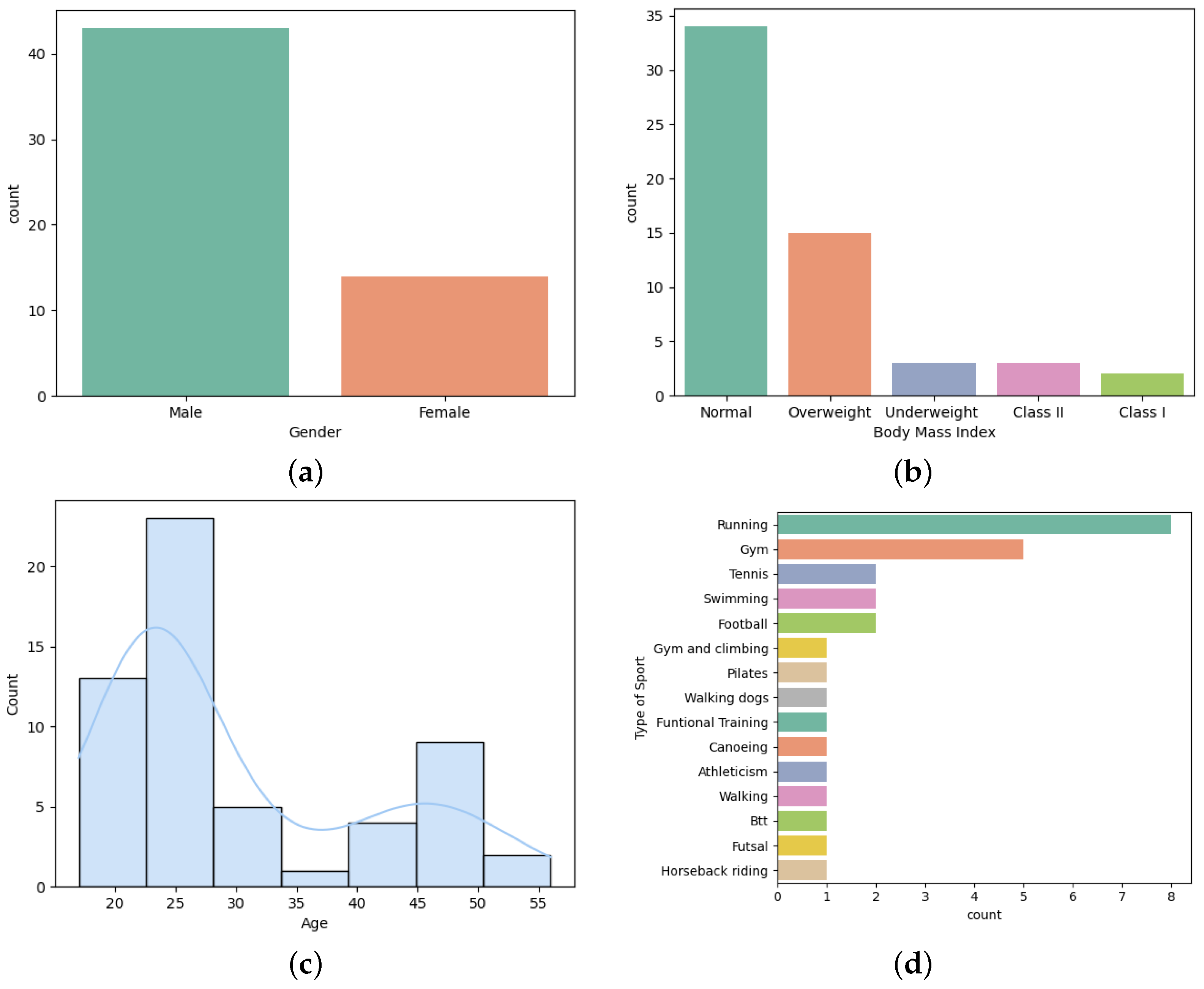
3.4. Participants Information

In order to perform the driving simulations, professors and research fellows, from the Polytechnic Institute of Cávado and Ave, were invited to participate in the experience. Fifty-seven people accepted to be part of this study. Most of the participants were male and, in terms of body mass index, were normal. Follow by overweight, underweight, class II ($35\le bmi<40$), and class I ($30\le bmi<35$). Moreover, there were participants from different age groups, ranging from 17 to 56 years old. According to the age distribution, Figure 3c, it is possible to identify that most of the participants were young. Furthermore, $50.88\%$ of them played sports, where running, going to the gym, tennis, swimming, and soccer were the most common.

There were only 14% of participants that present a health condition, with asthma (37.5%) and hypertension (25%) being the most common followed by type I diabetes (12.5%), myasthenia gravis (12.5%), and Gilbert syndrome (12.5%). In terms of sleep disorders, it was evaluated the risk of developing obstructive sleep apnea, the level of daytime sleepiness, sleep quality, and the circadian rhythm using the Stop-Bang, Epworth Sleepiness Scale, Pittsburgh Sleep Quality, and Morning-Eveningness questionnaires [28,29,30,31]. A few participants presented a high risk of developing obstructive sleep apnea (10.91%), excessive daytime sleepiness (40%), and bad sleep quality (25.45%). Moreover, most of them were neither morning nor evening type (70.91%), followed by morning (16.37%), evening (10.91%), and definitely evening type (1.82%).

It was also asked about some substances ingested and the existence of stress, in the 24 h, prior to the simulation. After analyzing the results achieved,

Table 1. Substances ingested or felt, in the 24 h, before the simulation.

	Drank Coffee	Had Medicine	Drank Alcohol	Smoke Cigarette	Felt Stress
No	24	45	5	53	41
Yes	33	12	52	4	16

, most of the participants drank coffee, did not ingest medicine, alcohol, or smoked, and did not experience stress.

The next answers were about the participant’s experience during the simulation. First, the participants were asked about some symptoms experienced, such as sickness, vision problems, headache, fatigue, itching eyes, concentration problems, and anxiety. They had to rate their intensity from 0 to 5, which corresponds to not at all to very much.

Table 2. Symptoms during the simulation.

Symptom	0	1	2	3	4	5
Sicken	45	9	0	1	2	0
Vision Problems	21	19	11	3	3	0
Headache	33	10	7	7	0	0
Fatigue	15	7	13	12	7	3
Itching Eyes	22	12	8	6	6	3
Concentrate Problems	12	16	11	7	9	2
Anxiety	38	8	5	3	2	1

presents the results achieved. It is perceptible that vision problems, fatigue, itching eyes, and concentration were the symptoms most felt throughout the simulation.

Another aspect to take into consideration is the vehicle experience. Thus, it was asked if the participant had any difficulties controlling the vehicle, had any accidents, and had difficulty recognizing potential obstacles and responding to them in a timely manner. In this last question, they had to rate their experience from 0, which represents not at all, to 5, which is very much. A large portion of the participants had no problems controlling the vehicle, although 40.37% did, and 56.14% had an accident. The difficulty in recognizing the obstacles was shown by 66.67% of the participants, although some had more problems than others.

The last questions were about the level of drowsiness, considering the Karolinska Sleepiness Scale, in which period of time they felt more drowsy (at the beginning, middle, or at the end of the simulation), if they felt more drowsiness during the night, and the level of difficulty to stay awake (0 representing none up to 5 representing a lot). Note that after the classification of the drowsiness level, the following questions were only presented to those who felt any signs of drowsiness. The levels considered were from “some signs of sleepiness” to “very sleepy, great effort to keeping awake, fighting sleep”.

Table 3. Karolinska Sleepiness Scale Results.

Level	Description	Count
1	Extremely alert	1
2	Very alert	1
3	Alert	5
4	Rather alert	9
5	Neither alert nor sleepy	5
6	Some signs of sleepiness	9
7	Sleepy, but no effort to keep awake	12
8	Sleepy, some effort to keep awake	11
9	Very sleepy, great effort keeping awake, fighting sleep	4

presents the results achieved using the Karolinska Sleepiness Scale, where 36 participants felt signs of drowsiness considering the levels from 6 to 9. Therefore, it is perceptible that most of the participants felt drowsy during the simulation.

In terms of which time period did the participants felt the most sleepy, the majority of them felt it in the middle of the simulation (80.56%), a few felt it at the end (13.89%), and only 5.55% at the beginning. Furthermore, it was consensual that during the night is when the greatest signs of drowsiness are felt (72.22%). Finally, none of the participants gave a score of 5 to how difficult it is to stay awake, and only 19.44% assigned a score of 4, 22.22% assigned a score of 2, and 3. These questions are self-reported and sometimes the answers are not in accordance with the video captured. For instance, there were a few participants that almost fell asleep during the simulation. This means that it was hard for them to keep their eyes open and, consequently, stay awake. Thereby, it was expected to have a level 5 for the difficulty of being awake.

After performing the classification of the drowsiness phases, by videoing the participant’s face, the percentages of each phase were extracted, taking into consideration Wierwille and Ellsworth’s drowsiness scale [16]. This scale divides drowsiness into five levels, from not drowsy (S1) to extremely drowsy (S5). Thus, Figure 4 presents the respective percentage for each level, globally. It is clearly perceptible that most of the participants did not reach level S5 since this level has lower variability (the difference between the 3rd and 1st quartile, also known as the interquartile range) when compared with the remaining levels. On the other hand, levels S1, S2, S3, and S4 present the greatest variability, where the interquartile range is 23.23, 27.86, 19.92, and 36.33, respectively.

4. Results

This section presents the heart rate variability metrics, for each domain, considered in the analysis. Then, the MSPC-PCA analysis was conducted for both heart rate variability and accelerometer information. Finally, it is discribed the out-of-control points analysis.

4.1. Variables Description

Heart rate variability is divided into time, frequency, and nonlinear domains, as was mentioned above. For each domain, there are different variables that can be computed, every two minutes. In terms of time, it was considered 16 variables, where 12 are related to the R-R intervals, and the remaining 4 are associated with the heart rate. Regarding the frequency and nonlinear domains, 5 and 4 variables were considered, respectively. All the variables used and the respective description is presented in 

Table 4. Heart Rate Variability Time Domain Metrics.

Domain	Metrics	Description
Time	mean_nni	Mean of the R–R intervals.
	median_nni	Median of the R–R intervals.
	range_nni	Difference between the maximum and the minimum of the R–R intervals.
	sdnn	Standard Deviation of the R–R intervals.
	sdsd	Standard deviation of differences between adjacent R–R intervals.
	rmssd	Square root of the mean of the sum of the squares of differences between adjacent R–R intervals.
	nni_50	Intervals’ number differences of successive R–R intervals greater than 50 ms.
	pnni_50	Derived Proportion by dividing nni_50 by the R–R intervals’ total number.
	nni_20	Intervals’ number differences of successive R–R intervals greater than 20 ms.
	pnni_20	Derived Proportion by dividing nni_20 by the R–R intervals’ total number.
	cvsd	rmssd divided mean_nni.
	cvnni	sdnn divided by mean_nni.
	mean_hr	Heart rate mean.
	min_hr	Heart rate minimum.
	max_hr	Heart rate maximum.
	std_hr	Standard deviation of the heart rate.
Frequency	power_vlf	Variance in HRV in the very low frequency.
	power_lf	Variance in HRV in the low frequency
	power_hf	Variance in HRV in the high frequency
	total_power	Total power density spectral.
	lf_hf_ratio	lf/hf ratio.
Non-Linear	csi	Cardiac Sympathetic Index.
	cvi	Cadiac Vagal Index.
	modified_csi	Modified csi.
	sampen	Sample entropy.

. A more detailed description of each variable can be found at [11].

4.2. MSPC-PCA Analysis

In order to identify the out-of-control points for both heart rate variability and accelerometer information, the MSPC-PCA was applied. The first step was to determine the time, frequency, nonlinear domain, and accelerometer principal component scores. Then, the Hotelling $T^2$, SPE statistics, and the upper limit control were assessed, considering the 95% confidence level, for each principal component. This analysis was conducted for all the participants, and since there are many graphs to display, for a better understanding of the proposed methodology, in this subsection, the analysis will only focus on participant 15.

Figure 5 presents the achieved out-of-control points for the time, frequency, and nonlinear principal components of the SPE (first line) and Hotelling $T^2$ (second line) statistics. With this visualization, the time and nonlinear domain components had one and two out-of-control points for the SPE and Hotelling $T^2$, respectively. The frequency domain component had only one out-of-control point for both statistics. Therefore, the heart rate variability at the time periods 1, 6, 7, 26, and 31 is out-of-control. Since the heart rate variability metrics were computed every two minutes, instant 1 represents the 2nd to 4th minutes of simulation. The instant 6 is the 12th to 14th minute and so on.

The same analysis was conducted for the accelerometer information, Figure 6, where it is noticeable that there are two out-of-control points in both statistics. Therefore, the time periods 0, 1, 20, and 37 are out-of-control considering the X, Y, and Z values of the accelerometer.

Overall, with the application of the MSPC-PCA methodology on the heart rate variability and accelerometer information, it was possible to identify 5 and 4 out-of-control points, respectively, where only one point is common for both data. Thus, it is important to understand what the out-of-control values represent and whether noise in the signal affects the points found in the heart rate variability or not.

The points achieved as out of control considering the heart rate variability and accelerometer, with the MSPC-PCA methodology, need to be carefully analyzed. This approach was evaluated for all participants; however, only the results for two participants (15 and 21) with different experiences will be presented (Figure 7). In the first line, the drowsiness periods reached using the MSPC-PCA, for the heart rate variability, are visible where the value 1 represents the out-of-control point, over the simulation time, in minutes. The out-of-control points using the accelerometer information were also added. In the second line, the drowsiness levels from Wierwille and Ellsworth’s drowsiness scale [16] are plotted over the simulation time.

It is noticeable that participant 21 has more transitions and reached higher levels of drowsiness than participant 15. Consequently, it also has more out-of-control points using the heart rate variability since, in the drowsiness periods, the value 1 was reached more often, which would be expected. In terms of the accelerometer, the first point, in both cases, is out of control, and it represents the first two minutes using the wearable device. During that time, the participants are adjusting the positioning of the device. It is also visualized that, for participant 15, there is one out-of-control point in common using the heart rate variability and accelerometer. Since this point happened before the recording of the participant’s face, it is not possible to check if there is a transition change and greater movement of the participant’s arm. This happened with other participants and the drowsiness transition is not affected by noise due to large movements.

Another aspect to take into account is that, for participant 15, any out-of-control point does not represent a drowsiness transition, considering the present drowsiness classification. This is contrary to participant 21 in which some transitions are, actually, being detected. For a better understanding of what is happening, what conclusions can be drawn, and what improvements can be implemented, it is necessary to evaluate the number of drowsiness levels transitions, the number of out-of-control points reached using the heart rate variability and accelerometer, and the number of out-of-control points in common (see Figure 8).

Globally, considering all the information from all the participants, there are 2 to 18 drowsiness transitions, where 7, 8, and 10 are the most common. However, there are 2 to 12 and 0 to 7 out-of-control points, using the multivariate statistical process control for the heart rate variability and accelerometer, respectively. The most common for the heart rate variability was between 6 to 9 points of control, whereas for the accelerometer, it was 2 to 4. When the number of out-of-control points reached in both sets of data are compared (in other words, the heart variability and accelerometer at the same time), there are 39.62% with 1 point in common, 11.32% with 2 points, and 7.55% with 3 or 4 points. This means that 41.51% does not have any point in common. The next step was to evaluate the presence of a transition in which the points are out of control due to both heart rate variability and accelerometer. Therefore, considering the results achieved, only 14.29% of the common out-of-control points actually have a drowsiness transition.

With this analysis, it is clear that improvements need to be made. Hence, the suggestion is to identify the out-of-control points for heart rate variability and compare them with the video in case of a transition; otherwise, check if it is possible to anticipate or delay a defined transition. Figure 9 presents the new drowsiness classification, for both participants 15 and 21, with the respective rectification. The blue line represents the first drowsiness classification, and the orange line is the improved classification using the methodology presented. For participant 15, the first three out-of-control points occurred before the video recording. In the last two points, it was possible to identify a drowsiness transition, and for that reason, the drowsiness classification was modified. When it comes to participant 21, only the first out-of-control point occurred before the video recording, and at the remaining points, there was also a transition from drowsiness.

To evaluate the proposed method’s performance, the precision and recall metrics were computed. Contextually, it is intended to check the ability of the out-of-control points to actually represent a drowsiness transition, which is known as precision. On the other hand, it is also intended to verify the ability to detect real drowsiness transitions, which represents the recall metric. So, precision and recall can be expressed as Equations (9) and (10), respectively.

$$\mathrm{Precision}={\displaystyle \frac{\mathrm{Out}\text{-}\mathrm{of}\text{-}\mathrm{Control}\mathrm{Point}\cap \mathrm{Real}\mathrm{Transitions}}{\mathrm{Total}\mathrm{Number}\mathrm{of}\mathrm{Out}\text{-}\mathrm{of}\text{-}\mathrm{Control}\mathrm{Points}}}$$

(9)

$$\mathrm{Recall}={\displaystyle \frac{\mathrm{Real}\mathrm{Transitions}\cap \mathrm{Out}\text{-}\mathrm{of}\text{-}\mathrm{Control}\mathrm{Point}}{\mathrm{Total}\mathrm{Number}\mathrm{of}\mathrm{Transitions}}}$$

(10)

The results achieved are presented in

Table 5. Precision and Recall Metrics.

Drowsiness Classification	Precision	Recall
First Classification [21]	0.37	0.21
Improved Classification	0.83	0.47

. For the first drowsiness classification, the precision and recall values were equal to $0.37$ and $0.21$, respectively. However, with the improved classification, precision was equal to $0.83$ and recall to $0.47$. It is perceptible that using the proposed methodology it was possible to improve the drowsiness classification and achieve better results.

5. Discussion

Focusing on the results achieved, in the previous section, it was possible to verify that most of the out-of-control points for the heart rate variability are not being influenced by signal noise. This was a concern in the study conducted in [20], where the addition of the accelerometer information was mentioned as future work.

Nevertheless, note that the drowsiness classification was made manually, considering the video recording and the participant’s behavior. This turned out to be subjective, and it is important to find solutions to combat this problem. A similar approach was used in [15], where two trained individuals classified separately the same videos. The classification, in the same period, was different such that it was necessary to evaluate and discuss it together. This is also a bit subjective since the opinion of one evaluator can influence the other. In [44], the drowsiness classification was made by the participant, after the simulation, considering the Karolinska Sleepiness Scale. This may be questionable as it is not always easy to classify our state of drowsiness through a video.

Other alternatives have emerged such as identifying the duration of the blink automatically and using blink metrics to classify the drowsiness phases [32,45]. In our experience, this may not be reliable since external factors influence the results. The algorithm can have several weaknesses that cannot be controlled such as wearing glasses, lighting, the participant’s facial movement, or even looking back. In addition, it is not always possible to calibrate the participant’s eyes well to extract reliable metrics.

Besides that, evaluating the out-of-control points reached using the heart rate variability, it was possible to improve the drowsiness classification methodology mentioned in [21]. It is essential to evaluate each out-of-control point obtained to prove if there is actually a drowsiness transition. This means that it always needs to be verified to see if such is happening, regardless of the participant in question. In mathematical terms, $83\%$ of the out-of-control points represent a drowsiness transition (precision value), and only $47\%$ of the drowsiness transitions are correctly detected (recall value), using the improved classification. However, if the method developed in [21] is considered, it reaches $37\%$ and $21\%$ for precision and recall metrics, respectively. With the proposed method, it is possible to counter most of the problems mentioned before using the MSPC-PCA methodology, and it is possible to clearly detect the drowsiness transitions. However, this method is not perfect, as it does not identify all the drowsiness transitions. However, regarding the performed analyses, whenever there is an out-of-control point, there is, in most of them, a drowsiness transition. That is a good achievement.

6. Conclusions

Drowsiness at the wheel is a topic of relevance since it reduces the driver’s reaction time, and that can lead quickly to road accidents. It can cause injuries or even the deaths of the drivers or those nearby. Therefore, it is important to take preventive measures that are not intrusive for the driver.

The aim of this work was the identification of a drowsiness transition method using the heart rate variability and accelerometer information through a wearable device. It is intended to identify the maximum number of drowsiness transitions and to reduce the identification of signal noise through driving simulations. This work contributes to the automatic detection of drowsiness transitions that is not influenced by external subjectivity and noise (from the signal or from large movements). It can be considered an unsupervised methodology and a low-cost system that is nonintrusive for drivers’ activity.

Driving simulations were developed with 57 people, in which most of them were male, with a normal body mass index, young, and fit. In terms of sleep disorders, a few participants presented a high risk of developing obstructive sleep apnea; they had excessive daytime sleepiness and bad sleep quality. Two interesting remarks are that most of the participants had an accident and had difficulties recognizing obstacles. It was also found that most participants experienced signs of drowsiness, and it was consensual that they occurred mostly in the middle of the night, during the simulation.

Therefore, multivariate statistical process control, using principal components analysis, was the method considered. Four main components were considered—the X, Y, and Z values of the accelerometer, time, frequency, and nonlinear domains of the heart rate variability. Then, the out-of-control points reached were analyzed, and it was possible to prove that most of the points of the heart rate variability were not being influenced by the external noise. Besides that, it was also possible to improve the drowsiness classification, previously defined using Wierwille and Ellsworth’s drowsiness scale. It was proved that most of the out-of-control points represent drowsiness transitions ($83\%$), and less than half of the drowsiness transitions are detected ($47\%$). Thus, the proposed method showed promising results for detecting drowsiness transitions and is not an intrusive alternative to the driver’s work functions.

The main limitation of the proposed work is the time consumption that is required since the process of classifying the drowsiness stages is not automatic. Moreover, it was not possible to detect all the drowsiness transitions and, for that reason, the recall value was low. Further analysis is needed to understand why in some participants few transitions are detected. Besides that, machine learning algorithms must be performed to classify the drowsiness state. The identification of the best subset of variables to classify the drowsiness transitions known as feature selection optimization is another type of analysis that could be performed. The implementation in a real context may also be something to consider.

References

1. Dernocoeur, K. Asleep at the wheel. Emerg. Med. Serv. 2000, 29, 32. [Google Scholar] [PubMed]
2. Kortelainen, J.M.; Mendez, M.O.; Bianchi, A.M.; Matteucci, M.; Cerutti, S. Sleep staging based on signals acquired through bed sensor. IEEE Trans. Inf. Technol. Biomed. 2010, 14, 776–785. [Google Scholar] [CrossRef] [PubMed]
3. Bendak, S.; Rashid, H.S. Fatigue in aviation: A systematic review of the literature. Int. J. Ind. Ergon. 2020, 76, 102928. [Google Scholar] [CrossRef]
4. Altevogt, B.M.; Colten, H.R. (Eds.) Sleep Disorders and Sleep Deprivation: An Unmet Public Health Problem; National Academies Press: Washington, DC, USA, 2006. [Google Scholar]
5. Moradi, A.; Nazari, S.S.H.; Rahmani, K. Sleepiness and the risk of road traffic accidents: A systematic review and meta-analysis of previous studies. Transp. Res. Part Traffic Psychol. Behav. 2019, 65, 620–629. [Google Scholar] [CrossRef]
6. Ramzan, M.; Khan, H.U.; Awan, S.M.; Ismail, A.; Ilyas, M.; Mahmood, A. A survey on state-of-the-art drowsiness detection techniques. IEEE Access 2019, 7, 61904–61919. [Google Scholar] [CrossRef]
7. Barr, L.; Popkin, S.; Howarth, H. An Evaluation of Emerging Driver Fatigue Detection Measures and Technologies; Technical report, United States; Department of Transportation, Federal Motor Carrier Safety: Washington, DC, USA, 2009. [Google Scholar]
8. Ingre, M.; Åkerstedt, T.; Peters, B.; Anund, A.; Kecklund, G. Subjective sleepiness, simulated driving performance and blink duration: Examining individual differences. J. Sleep Res. 2006, 15, 47–53. [Google Scholar] [CrossRef] [PubMed]
9. Bennett, M.S. Heart Rate Variability: Using Biometrics to Improve Outcomes in Trauma-Informed Organizations; A B.I.G. Publishing Project. 2020. Available online: https://www.scribd.com/book/469800653/Heart-Rate-Variability-Using-Biometrics-to-Improve-Outcomes-in-Trauma-Informed-Organizations (accessed on 20 January 2023).
10. Forcolin, F.; Buendia, R.; Candefjord, S.; Karlsson, J.; Sjöqvist, B.A.; Anund, A. Comparison of outlier heartbeat identification and spectral transformation strategies for deriving heart rate variability indices for drivers at different stages of sleepiness. Traffic Inj. Prev. 2018, 19, S112–S119. [Google Scholar] [CrossRef]
11. Shaffer, F.; Ginsberg, J.P. An overview of heart rate variability metrics and norms. Front. Public Health 2017, 5, 258. [Google Scholar] [CrossRef] [Green Version]
12. Stancin, I.; Cifrek, M.; Jovic, A. A review of EEG signal features and their application in driver drowsiness detection systems. Sensors 2021, 21, 3786. [Google Scholar] [CrossRef]
13. Iqbal, S.; Mahgoub, I.; Du, E.; Leavitt, M.A.; Asghar, W. Advances in healthcare wearable devices. NPJ Flex. Electron. 2021, 5, 1–14. [Google Scholar] [CrossRef]
14. Yan, C.; Coenen, F.; Yue, Y.; Yang, X.; Zhang, B. Video-based classification of driving behavior using a hierarchical classification system with multiple features. Int. J. Pattern Recognit. Artif. Intell. 2016, 30, 1650010. [Google Scholar] [CrossRef] [Green Version]
15. Kundinger, T.; Sofra, N.; Riener, A. Assessment of the potential of wrist-worn wearable sensors for driver drowsiness detection. Sensors 2020, 20, 1029. [Google Scholar] [CrossRef] [Green Version]
16. Strine, T.W.; Chapman, D.P. Associations of frequent sleep insufficiency with health-related quality of life and health behaviors. Sleep Med. 2005, 6, 23–27. [Google Scholar] [CrossRef] [PubMed]
17. Hoddes, E.; Zarcone, V.; Smythe, H.; Phillips, R.; Dement, W.C. Quantification of sleepiness: A new approach. Psychophysiology 1973, 10, 431–436. [Google Scholar] [CrossRef] [PubMed]
18. Weinbeer, V.; Muhr, T.; Bengler, K.; Baur, C.; Radlmayr, J.; Bill, J. Highly automated driving: How to get the driver drowsy and how does drowsiness influence various take-over-aspects? In Proceedings of the 8. Tagung Fahrerassistenz, München, Germany, 22–23 November 2017. [Google Scholar]
19. Abe, E.; Fujiwara, K.; Hiraoka, T.; Yamakawa, T.; Kano, M. Development of drowsiness detection method by integrating heart rate variability analysis and multivariate statistical process control. SICE J. Control Meas. Syst. Integr. 2016, 9, 10–17. [Google Scholar] [CrossRef] [Green Version]
20. Antunes, A.R.; Braga, A.C.; Gonçalves, J. Drowsiness detection using multivariate statistical process control. In Proceedings of the International Conference on Computational Science and Its Applications, Malaga, Spain, 4–7 July 2022; Springer: Berlin/Heidelberg, Germany, 2022; pp. 571–585. [Google Scholar]
21. Antunes, A.R.; Meneses, M.V.; Gonçalves, J.; Braga, A.C. An Intelligent System to Detect Drowsiness at the Wheel. In Proceedings of the 2022 10th International Symposium on Digital Forensics and Security (ISDFS), Istanbul, Turkey, 6–7 June 2022; pp. 1–6. [Google Scholar]
22. Ahmed, M.; Mahmood, A.N.; Hu, J. A survey of network anomaly detection techniques. J. Netw. Comput. Appl. 2016, 60, 19–31. [Google Scholar] [CrossRef]
23. Chandola, V.; Banerjee, A.; Kumar, V. Anomaly detection: A survey. ACM Comput. Surv. (CSUR) 2009, 41, 1–58. [Google Scholar] [CrossRef]
24. Ferrer, A. Multivariate statistical process control based on principal component analysis (MSPC-PCA): Some reflections and a case study in an autobody assembly process. Qual. Eng. 2007, 19, 311–325. [Google Scholar] [CrossRef]
25. MacGregor, J.F. Using on-line process data to improve quality: Challenges for statisticians. Int. Stat. Rev. 1997, 65, 309–323. [Google Scholar] [CrossRef]
26. Jackson, J.E.; Mudholkar, G.S. Control procedures for residuals associated with principal component analysis. Technometrics 1979, 21, 341–349. [Google Scholar] [CrossRef]
27. Alcala, C.F.; Qin, S.J. Analysis and generalization of fault diagnosis methods for process monitoring. J. Process Control 2011, 21, 322–330. [Google Scholar] [CrossRef]
28. Chung, F.; Abdullah, H.R.; Liao, P. STOP-Bang questionnaire: A practical approach to screen for obstructive sleep apnea. Chest 2016, 149, 631–638. [Google Scholar] [CrossRef] [Green Version]
29. Johns, M.W. A new method for measuring daytime sleepiness: The Epworth sleepiness scale. Sleep 1991, 14, 540–545. [Google Scholar] [CrossRef] [Green Version]
30. Buysse, D.J.; Reynolds, C.F., III; Monk, T.H.; Berman, S.R.; Kupfer, D.J. The Pittsburgh Sleep Quality Index: A new instrument for psychiatric practice and research. Psychiatry Res. 1989, 28, 193–213. [Google Scholar] [CrossRef]
31. Horne, J.A.; Östberg, O. Individual differences in human circadian rhythms. Biol. Psychol. 1977, 5, 179–190. [Google Scholar] [CrossRef]
32. Cech, J.; Soukupova, T. Real-time eye blink detection using facial landmarks. Cent. Mach. Percept. Dep. Cybern. Fac. Electr. Eng. Czech Tech. Univ. Prague 2016, 1–8. [Google Scholar]
33. Shafiq, M.; Gu, Z. Deep residual learning for image recognition: A survey. Appl. Sci. 2022, 12, 8972. [Google Scholar] [CrossRef]
34. Akhter, N.; Tharewal, S.; Gite, H.; Kale, K. Microcontroller based RR-Interval measurement using PPG signals for Heart Rate Variability based biometric application. In Proceedings of the 2015 International Conference on Advances in Computing, Communications and Informatics (ICACCI), Kochi, India, 10–13 August 2015; pp. 588–593. [Google Scholar]
35. Regalia, G.; Onorati, F.; Lai, M.; Caborni, C.; Picard, R.W. Multimodal wrist-worn devices for seizure detection and advancing research: Focus on the Empatica wristbands. Epilepsy Res. 2019, 153, 79–82. [Google Scholar] [CrossRef] [PubMed]
36. Bindu, K.H.; Raghava, M.; Dey, N.; Rao, C.R. Coefficient of Variation and Machine Learning Applications; CRC Press: Boca Raton, FL, USA, 2019. [Google Scholar]
37. VanRossum, G.; Drake, F.L. The Python Ladnguage Reference; Python Software Foundation: Amsterdam, The Netherlands, 2010. [Google Scholar]
38. McKinney, W. Pandas: A foundational Python library for data analysis and statistics. Python High Perform. Sci. Comput. 2011, 14, 1–9. [Google Scholar]
39. Ari, N.; Ustazhanov, M. Matplotlib in python. In Proceedings of the 11th International Conference on Electronics, Computer and Computation (ICECCO), Abuja, Nigeria, 29 September–1 October 2014; pp. 1–6. [Google Scholar]
40. Taskesen, E. pca: A Python Package for Principal Component Analysis. 2020. Available online: https://erdogant.github.io/pca (accessed on 28 March 2022).
41. Harris, C.R.; Millman, K.J.; Van Der Walt, S.J.; Gommers, R.; Virtanen, P.; Cournapeau, D.; Wieser, E.; Taylor, J.; Berg, S.; Smith, N.J.; et al. Array programming with NumPy. Nature 2020, 585, 357–362. [Google Scholar] [CrossRef]
42. Virtanen, P.; Gommers, R.; Oliphant, T.E.; Haberland, M.; Reddy, T.; Cournapeau, D.; Burovski, E.; Peterson, P.; Weckesser, W.; Bright, J.; et al. SciPy 1.0: Fundamental algorithms for scientific computing in Python. Nat. Methods 2020, 17, 261–272. [Google Scholar] [CrossRef] [PubMed] [Green Version]
43. Waskom, M.L. Seaborn: Statistical data visualization. J. Open Source Softw. 2021, 6, 3021. [Google Scholar] [CrossRef]
44. Leng, L.B.; Giin, L.B.; Chung, W.Y. Wearable driver drowsiness detection system based on biomedical and motion sensors. In Proceedings of the 2015 IEEE Sensors, Busan, Korea, 1–4 November 2015; pp. 1–4. [Google Scholar]
45. Choi, M.; Koo, G.; Seo, M.; Kim, S.W. Wearable device-based system to monitor a driver’s stress, fatigue, and drowsiness. IEEE Trans. Instrum. Meas. 2017, 67, 634–645. [Google Scholar] [CrossRef]
Figure 1. Driving Simulation Procedure.
Applsci 13 02651 g001
Figure 2. Analysis Procedure Flowchart.
Applsci 13 02651 g002
Figure 3. Personal information: (a) Gender. (b) Body mass index. (c) Age. (d) Type of sports.
Applsci 13 02651 g003
Figure 4. Percentage of Each Drowsiness Scale.
Applsci 13 02651 g004
Figure 5. Participant 15 MSPC-PCA Analysis for the Heart Rate Variability.
Applsci 13 02651 g005
Figure 6. Participant 15 MSPC-PCA Analysis for the Accelerometer information.
Applsci 13 02651 g006
Figure 7. MSPC-PCA Methodology and Drowsiness Classification. (a) participant 15. (b) participant 21.
Applsci 13 02651 g007
Figure 8. Transitions and Out-of-Control Points (a) Number of Drowsiness Transitions. (b) Heart Rate Variability Out-of-Control Points. (c) Accelerometer Out-of-Control Points. (d) Out-of-Control Points in Both Heart Rate Variability and Accelerometer.
Applsci 13 02651 g008
Figure 9. Drowsiness Classification Improvements. (a) participant 15. (b) participant 21.
Applsci 13 02651 g009