An Efficient Feature Augmentation and LSTM-Based Method to Predict Maritime Traffic Conditions

Abstract

The recent emergence of futuristic ships is the result of advances in information and communication technology, big data, and artificial intelligence. They are generally autonomous, which has the potential to significantly improve safety and drastically reduce operating costs. However, the commercialization of Maritime Autonomous Surface Ships requires the development of appropriate technologies, including intelligent navigation systems, which involves the identification of the current maritime traffic conditions and the prediction of future maritime traffic conditions. This study aims to develop an algorithm that predicts future maritime traffic conditions using historical data, with the goal of enhancing the performance of autonomous ships. Using several datasets, we trained and validated an artificial intelligence model using long short-term memory and evaluated the performance by considering several features such as the maritime traffic volume, maritime traffic congestion fluctuation range, fluctuation rate, etc. The algorithm was able to identify features for predicting maritime traffic conditions. The obtained results indicated that the highest performance of the model with a valid loss of 0.0835 was observed under the scenario with all trends and predictions. The maximum values for 3, 6, 12, and 24 days and the congestion of the gate lines around the analysis point showed a significant effect on performance. The results of this study can be used to improve the performance of situation recognition systems in autonomous ships and can be applied to maritime traffic condition recognition technology for coastal ships that navigate more complex sea routes compared to ships navigating the ocean.

1. Introduction

The application of information and communication technology, big data, and artificial intelligence technology to the conventional concept of ships has led to the emergence of futuristic ships, which are safer and more efficient compared to conventional ships. In general, futuristic ship refers to a Maritime Autonomous Surface Ship that can navigate without intervention from the crew. Thus far, several countries have implemented policy support and government-led projects to preempt the autonomous ship industry. In South Korea, the “autonomous ship technology development project” is being jointly conducted by the Ministry of Oceans and Fisheries and the Ministry of Trade, Industry, and Energy.

In the commercialization of autonomous ships, it is necessary to develop appropriate technologies including Intelligent navigation systems, Engine automation systems, Performance verification center and verification technology, and Operation technology and standardization, which represent the core components of the ‘Intelligent navigation system’ that will replace navigators and captains.

The ‘Intelligent navigation system’ consists of situation recognition of maritime traffic conditions, generation and following of routes, collision avoidance, and returning routes. The situation recognition of maritime traffic conditions involves the identification of the current traffic conditions and the prediction of future traffic conditions. This is a prior technology that is essential to ensure the safe navigation of autonomous ships. Situation recognition technology for determining maritime traffic conditions generally involves the use of cameras or the identification of the current maritime traffic conditions based on traffic data. This aspect is a critical component in the development of route generation algorithms or the collision avoidance algorithms of autonomous ships.

In the process of recognizing a situation, navigators predict future maritime traffic conditions using empirical and intuitive judgment based on traffic data in addition to a visual assessment of traffic conditions. Based on these factors, decisions are made regarding the safety of a route and collision avoidance. Therefore, for an autonomous ship to generate a safer route and to efficiently perform collision avoidance considering future maritime traffic conditions, it is necessary to predict future maritime traffic conditions as well as to assess current conditions.

Consequently, in this study, we aimed to develop an algorithm that predicts future traffic conditions based on past traffic data to improve the performance of the recognition system of autonomous ships. It was determined that the developed algorithm can be used not only to improve the recognition system of autonomous ships but can also be applied to maritime traffic condition recognition for coastal ship navigation along complex routes.

The Main Contributions of the paper are as follows:

• Development of an intelligent LSTM-based prediction algorithm for Maritime Traffic Conditions;
• Feature Augmentation for maritime traffic congestion;
• Utilizing large amount of data for traffic conditions;
• Motivation to develop Maritime Autonomous Surface Ships;
• Development of an Intelligent navigation system.

The rest of the paper is structured as follows: We briefly discuss the related work in Section 2, where we discussed different kind of maritime traffic condition predictions with linear and nonlinear methodologies. In Section 3, we discussed the theory of maritime traffic conditions. In Section 4, the LSTM and feature augmentation-based prediction algorithm of maritime traffic condition is discussed in detail with experimental results. In Section 5, the algorithm’s validation is given. Finally, the conclusions are drawn in Section 6.

2. Related Work

The prediction of maritime traffic conditions is one of the most challenging tasks, especially when talking about Maritime Autonomous Surface Ships. The automation challenges may vary depending on the scenario between land and sea. Vehicles on the road or highways usually travel in a lane; if we consider ships, they can travel in any direction depending on the sea currents’ directions. Furthermore, compared to the vehicle traffic regulations, the Convention on the International Regulations for Preventing Collisions at Sea (COLREGs) is dependent upon the operator experience, which is less accurately codified. Consequently, exertion will be increased to predict a ship’s behavior.

The studies about prediction of maritime traffic conditions are based on trajectory prediction and index prediction. The linear model of trajectory prediction can deal with the prediction of trajectories when the ship sails straight; these linear models (LM) are called constant velocity models (CVM). For Example, Perera and Soares [1] proposed an ocean vessel trajectory prediction based on an Extended Kalman filter with a curvilinear motion model with the measurements by a linear position model. Pallotta et al. [2] proposed an Ornstein–Uhlenbeck process based on control theory, and the method was based on the OU stochastic process used for ship prediction. Historical patterns of life estimated the parameters. Millefiori et al. [3] proposed a novel technique for long-term target state prediction, and the method is based on Stochastic Mean-Reverting Process. Sang et al. [4] developed a three-step closest point of approach (CPA) search method to accurately predict the ship’s future trajectory. The AIS data used in this paper were based on the Speed Over Ground (SOG), Course Over Ground (COG), Change of Speed (COS), and rate of turn (ROT) data. However, the prediction model’s accuracy depends on the label and physical knowledge recognition. Jaskolski [5] proposed a discrete Kalman filtering algorithm for dynamic data estimation to estimate the missing ship’s position distribution of trajectory points linearly. Zhang et al. [6] solved a trajectory prediction problem with wavelet analysis; the state transition model they used is based on the Hidden Markov Model to accurately predict the ship’s future position and large ship trajectory by constructing a Markov chain.

Currently, for predictive traffic management and monitoring, Kongsberg’s C-SCOPE solution [7] is the current commercial production system mainly dependent on linear models. Nevertheless, the LM-based techniques perform uncertainly when the vessel wants to change speed or course and tend to drift under specific conditions. Consequently, to overcome these limitations of linear models, many papers presented nonlinear models to enhance prediction accuracy.

The conventional nonlinear marine dynamics [8] utilized machine learning and deep learning [9]. However, each ML and DL strategy has different benefits and applications. Sometimes ML makes good predictions, while deep learning is time and space-consuming. On the other hand, deep learning is outstanding for large amounts of data, and outperforms ML models. Zandipour et al. [10] proposed an enhanced neurobiological-inspired algorithm, which takes real-time maritime tracking data to learn motion pattern models for situation awareness. Xiaopeng et al. [11] proposed a combination of grey prediction and an improved Markov model for island vessel trajectory prediction based on AIS data. Qi and Zheng [12] presented a machine learning and data mining-based vessel trajectory prediction. The main algorithm they used is a support vector machine (SVM) to cluster trajectories and classify them. Zhang et al. [13] proposed a big data analytics method to evaluate ship grounding risk in actual environmental circumstances, and they also applied big data on AIS nowcast data. Zhao et al. [14] presented an ensemble machine-learning framework for basic AIS data cleaning and removed all outliers in the data. The clean data are used to predict trajectory variation tendency in ships. The method is verified with three ship trajectory segments. Tu et al. [15] did a comprehensive survey from data to methodology and argued that new algorithms must be developed for accurate maritime traffic conditions. Most of the present path prediction algorithms are built on a fast update prediction method such as the Kalman filter. Due to the popularity and advancement of deep learning methods [16], efficient data-driven methods are becoming increasingly popular among researchers.

The index prediction includes predicting quantitative indicators expressing various maritime traffic conditions, including congestion, density, risk of collision, predicting maritime accidents, and so on. Son et al. [17] proposed a method that predicted maritime traffic congestion by combining the automatic identification systems of ships and port management information data. Ramin et al. [18] used timeseries models and the associative models to predict the maritime traffic density of Port Klang and the Straits of Malacca. For the prediction of maritime traffic flow, Zhou et al. 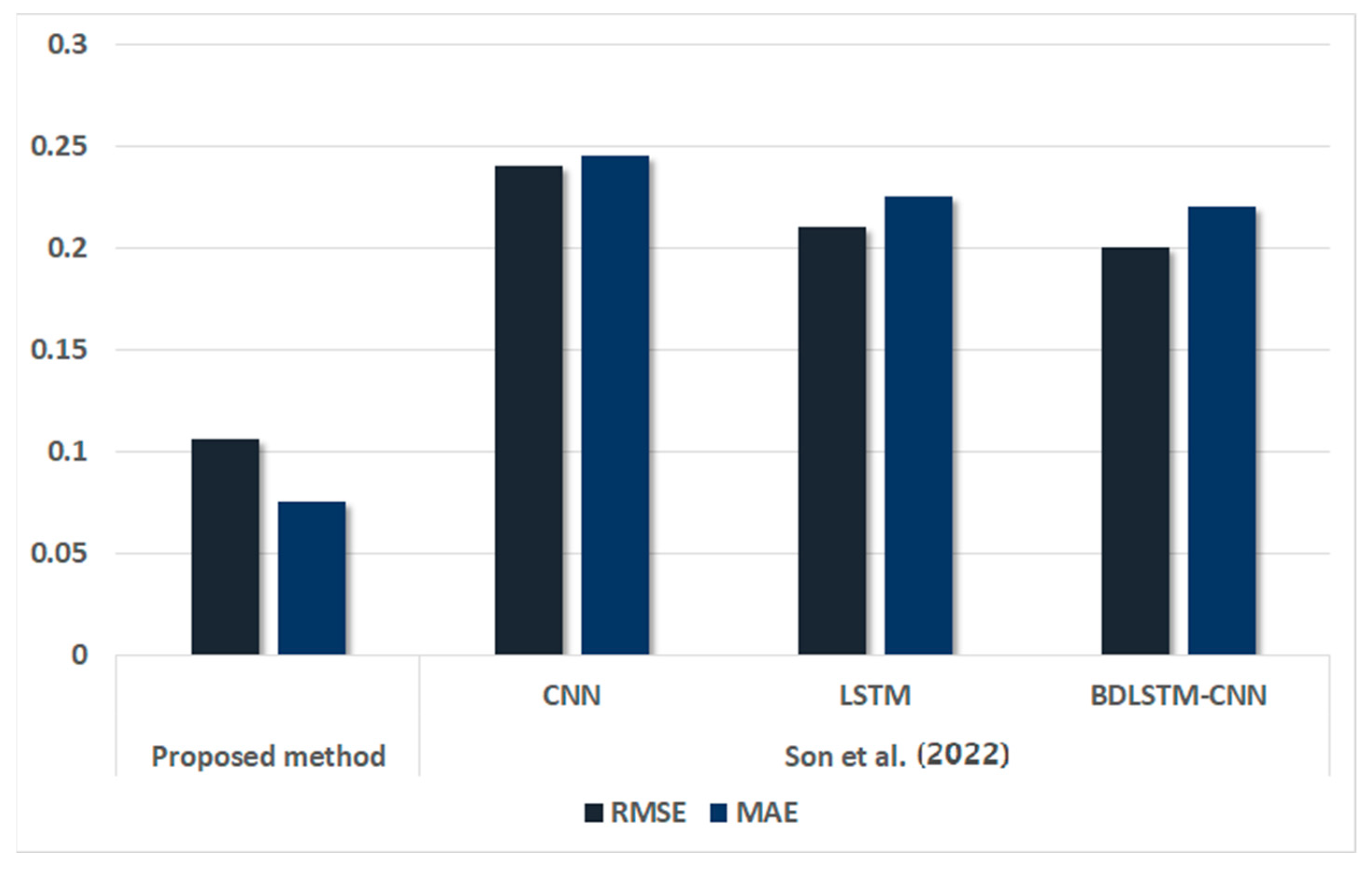[19] used deep learning solutions such as CNN, LSTM, and BDLSTM-CNN. Zhang et al. [20] used an improved PSO-BP mechanism which is a self-adaptive particle swarm optimization-back propagation. Lastly, Liang et al. [21] used a Spatio-Temporal Multigraph Convolutional Network to achieve fine-grained vessel traffic flow prediction.

In order to prevent marine accidents, the possibility of maritime accidents can be predicted, and there is also a method of predicting the risk of collision, which is the main cause of marine accidents. Liu et al. [22] and Namgung and Kim [23] proposed the system to predict regional collision risk using the Density-Based Spatial Clustering of Applications with Noise (DBSCAN) technique and a Recurrent Neural Network (RNN). To predict maritime accidents, Yang et al. [24] used Machine learning (ML) technology such as the random forest (RF) model, Adaboost model, gradient boosting decision tree (GBDT) model, and Stacking combined model and compared the result. Otay and Özkan [25] proposed a stochastic model using the geographical characteristics of the Istanbul strait and visualized risk map. There are studies that have used modern AI algorithms to make predictions; Abdel-Razek et al. [26] used Artificial Intelligence to improve energy efficiency in buildings. The focus of the article is on the implementation of an AI model that predicts room occupancy based on thermal comfort parameters such as temperature, humidity, and air velocity. Imran et al. [27] focused on the application of artificial intelligence techniques for predicting and detecting marine corrosion. They present case studies and experimental results to demonstrate the efficacy of these techniques in detecting and predicting marine corrosion and conclude that the application of artificial intelligence has the potential to revolutionize the field of marine corrosion prediction and detection. El Mekkaoui et al. [28] propose an algorithm that predicts future ship speed based on past data using a deep learning model. They also perform linear interpolation to handle missing data and apply feature augmentation to improve the performance of the model. The results of the study show that the proposed algorithm outperforms existing methods in terms of prediction accuracy.

In the above related studies, there was no study to identify which feature affected the prediction of maritime traffic congestion. Therefore, in this study, we tried to find the significant features for predicting maritime traffic congestion through feature augmentation and build a prediction algorithm of maritime traffic congestion using LSTM.

3. Maritime Traffic Conditions

Maritime traffic conditions refer to the comprehensive state of ship operators, ships, and the environment that constitute maritime traffic, and there are various ways to express them using quantitative indicators.

Maritime traffic congestion is an index that can be expressed as the percentage of the actual maritime traffic volume against the maritime traffic volume of a navigational passage. It is often used as a simple indicator of the average traffic volume and congestion of a navigational passage [29,30]. Maritime traffic congestion is also used as an index to select traffic conditions to evaluate the efficacy of the collision avoidance algorithms of autonomous ships [31]. Equation (1) is an expression for calculating maritime traffic congestion.

$$T_c \left(\%\right)=\frac{Q_t}{Q_p}·100\left(\%\right)$$

(1)

where

• $T_c$ = Maritime traffic congestion,
• $Q_t$ = Actual maritime traffic volume,
• $Q_p$ = Practical maritime traffic volume.

Since the area required for safe navigation of a vessel is usually proportional to the squared length of the ship, the actual maritime traffic volume is the summation of the length squared conversion traffic volumes by tonnage group, which is calculated as the product of number of ships and the length squared coefficient. Equations (2) and (3) are the expressions for calculating actual maritime traffic volume and length squared conversion traffic volume.

$$Q_t=\frac{{\sum }_{n=1}^m{V}_n}{D·T}$$

(2)

where

• $V_n$ = Length squared conversion traffic volume by tonnage group,
• $D$ = Port operation day,
• $T$ = Port operation time,
• $m$ = Number of tonnage group.

$$V_n=N_n·\left(L_n{}^2\right)$$

(3)

where

• $N_n$ = Number of ships by tonnage group,
• $L_n$ = Length coefficient by tonnage group.

Length coefficient is ratio of the representative length to the standard length of ships, representative length of ships is proportional to the cube root of average tonnage of ships, and standard length of ships is a weighted average of the representative length of ships by tonnage group. Equations (4) and (5) are the expressions for calculating length and representative length of ships.

$$L_n=\frac{R_n}{S}$$

(4)

where

• $R_n$ = Representative length of ships by tonnage group,
• $S$ = Standard length of ships.

$$R_n=\sqrt[3]{250·A{T}_n}$$

(5)

where

• $A{T}_n$ = Average tonnage of ships by tonnage group.

Practical maritime traffic volume is the value obtained by multiplying the maximum maritime traffic volume by the practical maritime traffic capacity coefficient, and the practical maritime traffic capacity coefficient generally has a value of 0.2 to 0.25. This refers to the practically allowable traffic volume depending on sea and weather conditions, maritime traffic conditions, and maritime traffic management methods, which means that it is 20 to 25% of the maximum maritime traffic volume. Equation (6) is an expression for calculating practical maritime traffic volume.

$$Q_p=Q_m·C_p$$

(6)

where

• $Q_m$ = Maximum maritime traffic volume,
• $C_p$ = Practical maritime traffic volume coefficient.

Maximum maritime traffic volume is a theoretical value that can be accommodated on a passage of width $W$, assuming that ships of a certain size are continuously navigating at speed $V$. The size of the ship is determined by the elliptical ship domain, which is the area necessary for the ship to navigate safely, and $\alpha$ and $\beta$ mean the major and minor axes of the ship domain. There are many theories about the shape and size of a ship domain, the elliptical ship domain is common. $\alpha$ usually has a value of 6.0 to 8.0 and $\beta$ has a value of 1.6 to 3.2. Equation (7) is an expression for calculating maximum maritime traffic volume.

$$Q_m=\frac{W·V}{\alpha ·\beta ·S^2}$$

(7)

where

• $W$ = Width of passage,
• $V$ = Velocity of ship,
• $\alpha$ = Major axis coefficient,
• $\beta$ = Minor axis coefficient.

Meanwhile, maritime traffic density is a metric that represents the number of navigation units per unit area that exists in an arbitrary period, as opposed to evaluating only the traffic capacity, which is the number of navigation units per arbitrary unit area per hour. Based on the evaluation of maritime traffic density, it is possible to derive a result considering the frequency of the navigating ships (${\mathsf{\rho }}_1$) and the occupied area of navigating ships (${\mathsf{\rho }}_2$) within a gridded sector [32]. Maritime traffic density is also used as an indicator in the design of coastal routes [33].

In addition, there is a potential assessment of the risk model, which is an index that includes the subjective risk of ship operators considering the overall condition of the ship and the environment [34]. It is also used in the development of collision risk notification algorithms for small ships [35].

Various quantitative methods for expressing maritime traffic conditions have different contents, depending on each method, and they must be utilized in compliance with the characteristics of the sea area and the purpose of the review.

This study aimed to develop a future maritime traffic condition prediction algorithm for maritime traffic congestion using the quantitative indicators for maritime traffic conditions adopted in the Guidelines on Maritime Traffic Safety Audit in accordance with the Maritime Safety Act in South Korea [36], which is to evaluate the safety of all types of port and water facilities in relation to ships’ passages.

4. Prediction Algorithm of Maritime Traffic Condition

4.1. Construction

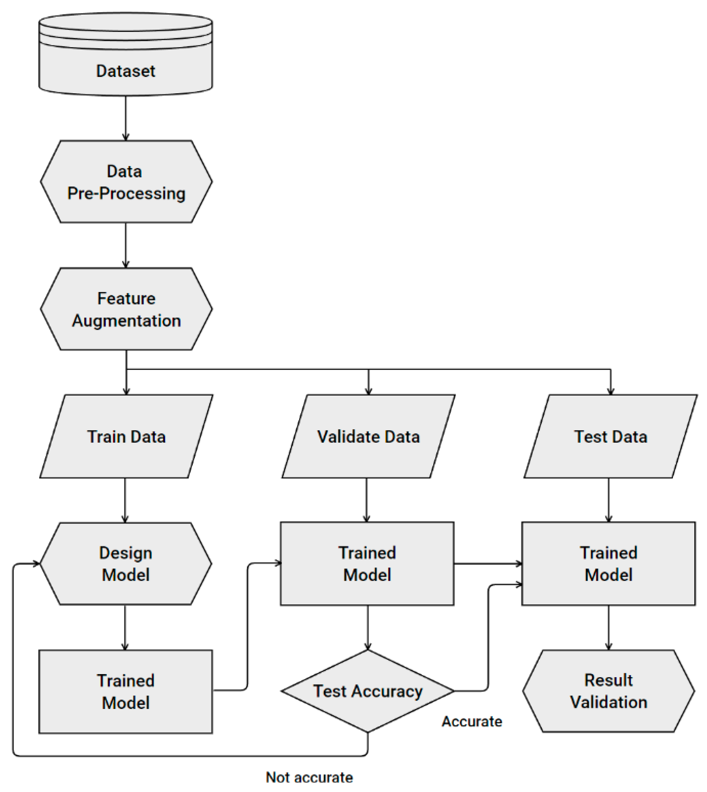
The construction process of the artificial intelligence algorithm consisted of 6 steps: obtaining the dataset, data pre-processing, feature augmentation, model design, training/validation of the model, and results validation. Figure 1 shows a construction diagram of the algorithm.

The dataset used in this study included the data from the automatic identification system (AIS). AIS is an important equipment required for ship operation, such as monitoring ship operation and identifying safe navigation conditions. According to the International Convention for the Safety of Life at Sea (SOLAS), it is compulsory to install AIS on all passenger ships and sailing ships with a gross tonnage of 300 tons or more.

Data pre-processing refers to the process of creating a shape suitable for data analysis and processing, and generally interpolates missing data or processes erroneous data. No matter how good the tool or analysis technique is, it is difficult to obtain good results with low-quality data, so about 80% of the total time is usually spent on data pre-processing. In the data pre-processing step, a range was selected according to the characteristics of the maritime traffic data, and pre-processing was performed using the interquartile range (IQR).

Similar to data augmentation, feature augmentation is an operation of extracting features by processing original data using domain knowledge. In the feature augmentation step, various features were obtained from the basic features to increase the prediction reliability for maritime traffic congestion.

Considering that maritime traffic data are time-series data, the long short-term memory (LSTM) model was used, which is a representative model for processing time-series data.

4.2. Data Preparation

Preparation of the data involves obtaining a dataset and pre-processing the data. There are various data related to maritime traffic conditions such as AIS, V-PASS, and LTE-M. AIS data are for ships with a gross tonnage of 300 tons or more. In addition, V-PASS data are data for fishing boats, and LTE-M data are provided from a wireless communication network that introduces LTE communication technology to the sea as a basis for providing intelligent maritime traffic information to ships sailing up to 100 km from the coast of Korea. However, personal access to LTE-M data is limited. Considering this comprehensively, AIS data were used in this study. AIS data were collected using AIS transponder capable of collecting both A class and B class, and position reports messages, ship static and voyage-related data messages were used. In addition, coordinate transformation was not performed for gate line analysis using WGS-84(World Geodetic System-84) based software (XTSSRC_v1.0).

Table 1. Description of dataset.

	Static Data	Dynamic Data
Size	8.22 MB	558 GB
Number of records	142,160	8,259,187,180
Type of information	Maritime Mobile Service Identity number (Integer), Ship’s name (Text), Ship’s type code (Integer), International Maritime Organization number (Integer), Call sign (Text), Length of all (Integer), Breath (Integer), Draft (Integer).	Maritime Mobile Service Identity number (Integer), Latitude (Double), Longitude (Double), Course of ground (Float), Speed of ground (Float), Heading (Integer), Time (DateTime).

is the description of the dataset.

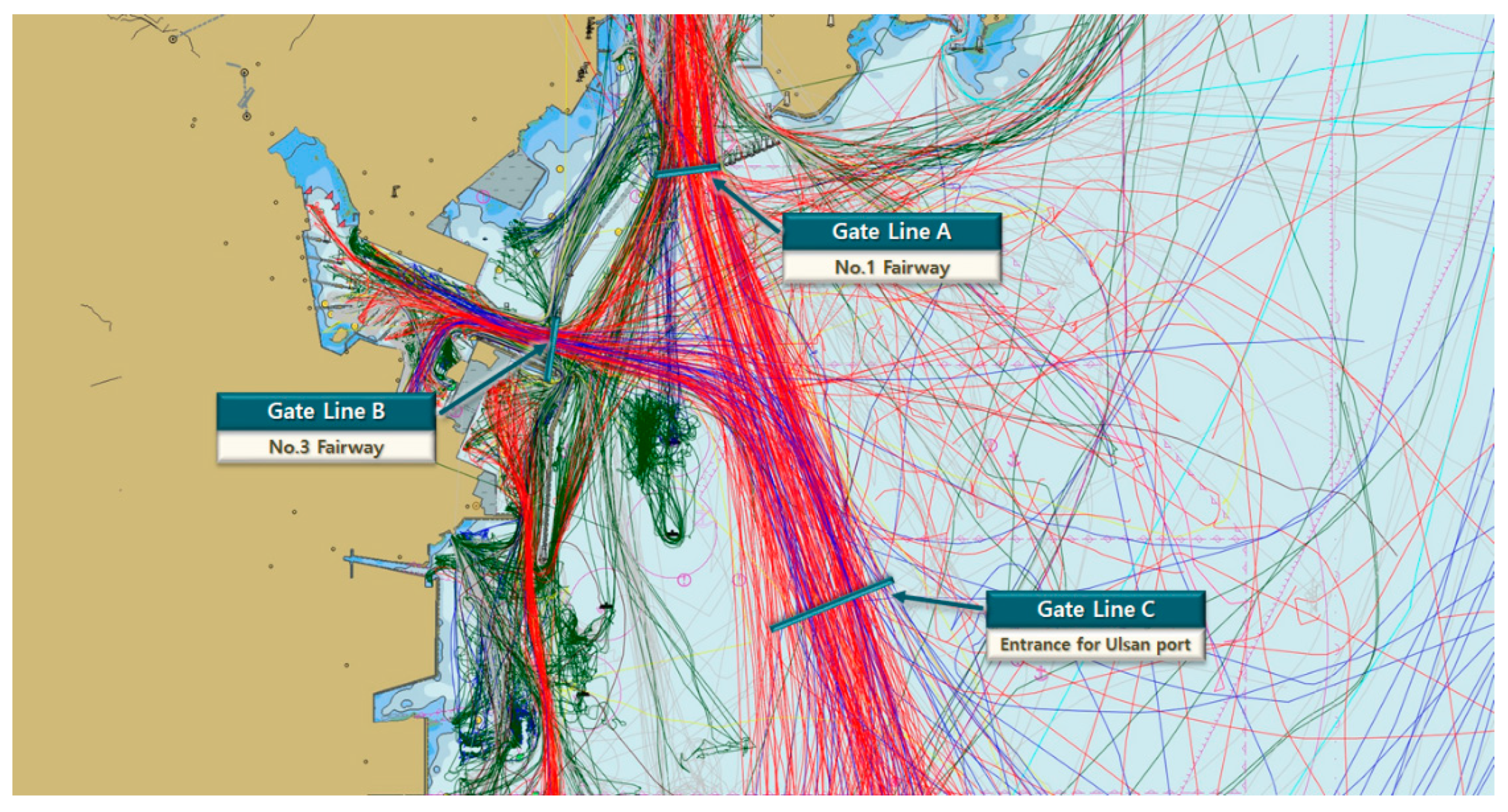
The target sea area was limited to Ulsan Port, the largest industrial support port in Korea; there are several fairways including the entrance for Ulsan Port. Among those, the most complicated gate line of No.1 Fairway was selected as the analysis point, which is near the gate line of No.3 Fairway and the entrance for Ulsan Port. The period of the data is from 1 September 2019 to 31 August 2020. Figure 2 is an example of the visualization of the AIS data of the target sea area.

Data pre-processing is a process that increases the reliability of data and is a very important step since it directly affects training results.

The AIS data consisted of dynamic, static, navigation-related, and safety-related information. Except for the dynamic information, the reception period of the remainder was 6 min, and the reception period of dynamic information changed from a minimum of 2 s to a maximum of 3 min, depending on the class of the AIS equipment and the dynamic condition of the ship. The occurrence of missing data was addressed through the implementation of linear interpolation. Moreover, a large number of outliers was present depending on the marine conditions and the communication environment, and these errors were addressed during the data pre-processing process.

The range of outliers was first selected by considering the characteristics of the target sea area. Outliers were removed using the IQR (interquartile range), which is the difference between the values in the top 75% and bottom 25% of the quartile. Equations (8) and (9) are expressions for calculating outliers using IQR.

$$\mathrm{IQR}=Q_3-Q_1$$

(8)

$$\{a | \left[a<\left(Q_1-1.5·\mathrm{IQR}\right)\right]\cup \left[a>\left(Q_3+1.5·\mathrm{IQR}\right)\right]\}$$

(9)

where

• $Q_1$: Midpoint of the lower half of the data values,
• $Q_2$: Midpoint of the upper half of the data values.

4.3. Feature Augmentation

There are many factors to be considered when predicting maritime traffic. The main factors include the number of ships and the maritime traffic volume, among others. Additionally, there are other factors such as weather conditions, waves, tidal and surface currents, the depth of water, the shape of the seabed as obtained from electronic navigational charts, and maritime traffic regulations, including port speed limits.

Features for predicting maritime traffic congestion include the predicted values of the number of ships and the maritime traffic volume, which means length squared conversion traffic volume; however, more features are required for a highly reliable prediction. Therefore, new features were obtained from the existing features through feature augmentation to improve the performance of the developed algorithm. Feature augmentation is a technique used in machine learning to increase the size of the dataset. It is achieved by generating new instances of the data using transformations or operations that preserve the underlying structure of the data. These new instances are combined with the original data to create a larger dataset that can be used to train a machine learning model.

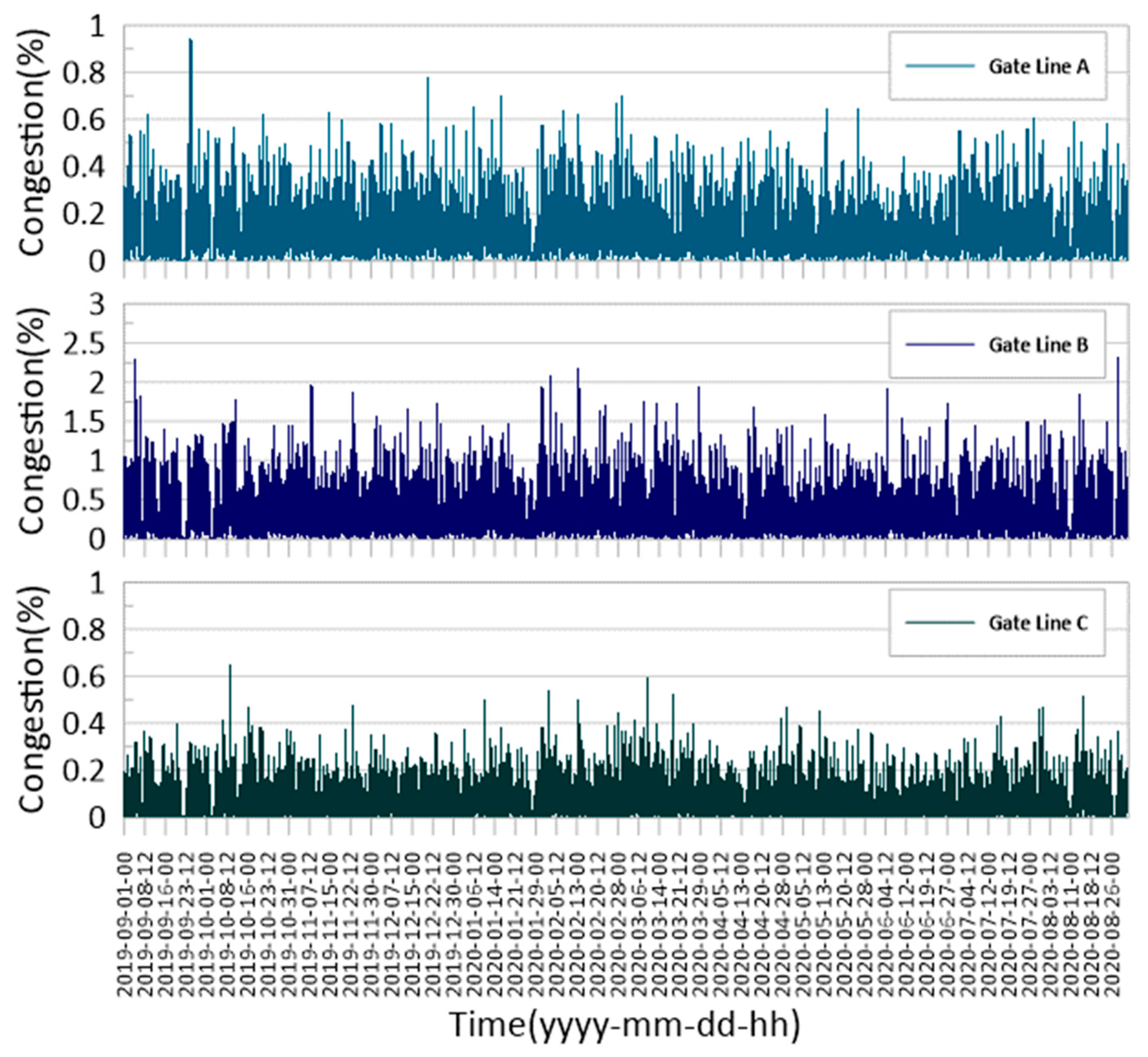
The maritime traffic congestion variance width; variance rate; variance probability; 3-day, 6-day, 9-day, and 24-day averages; and maximum maritime traffic congestion were selected as features in addition to the number of ships and maritime traffic volume. The maritime traffic congestion of major gate lines around the target gate line was additionally selected. The annual average was found to be 11.3% and the maximum value was 94.4%, when the maritime traffic congestion of gate line A (No. 1 fairway) was analyzed. The monthly average was the lowest in June (9.4%) and the highest in February (12.9%).

The annual average was found to be 30.2% and the maximum value was 230.9% when the maritime traffic congestion of gate line B (No. 3 fairway)—a major gate line around the target gate line—was analyzed. The monthly average was the lowest in September (28.3%) and the highest in March (33.2%). The annual average was found to be 6.7% and the maximum value was 65.3% when the maritime traffic congestion of gate line C (entrance to Ulsan Port) was analyzed. The monthly average was the lowest in June (5.5%) and the highest in March (8.1%). Figure 3 and Figure 4 show the hourly and monthly maritime traffic congestion analysis results by each gate line.

Among the features, the variance refers to the numerical expression of the degree of change in maritime traffic congestion over a certain period. The variance analysis includes the variance width, variance rate, and variance probability.

The variance width is used to obtain the magnitude of the average change in time-series data; it has the benefit of obtaining estimates on a non-parametric scale because no specific distribution is assumed. It is obtained using

$$\frac{1}{\left(n-1\right)}\hspace{1em}\hspace{1em}{\sum }_{t=1}^n\left(T_c\left(t\right)-T_c\left(t-1\right)\right)$$

(10)

The variance rate is the ratio between the variance width and the maritime traffic congestion value, and it is expressed as

$$\frac{\frac{1}{n} {\sum }_{t=1}^n{T}_c\left(t\right)}{ \frac{1}{\left(n-1\right)} {\sum }_{t=1}^n\left(T_c\left(t\right)-T_c\left(t-1\right)\right)}$$

(11)

The variance probability is expressed in binary notation by comparing the variance width with the maritime traffic congestion value. The variance probability is calculated using

$$\frac{\left(n-1\right)-\alpha }{\left(n-1\right)}$$

(12)

$$a=\left(n-1\right)-{\sum }_{t=1}^n\left(T_c\left(t\right)-T_c\left(t-1\right)\right)$$

$${\gamma }_n=\left\{\begin{array}{ll}1& ,T_c\left(t\right)>F_{range}\\ 0& ,T_c\left(t\right)\le F_{range}\end{array}\right.$$

(13)

where

• $\alpha$ = Coefficient of inclusion of fluctuation range considering the period,
• ${\gamma }_n$ = Specifies whether the fluctuation range is included.

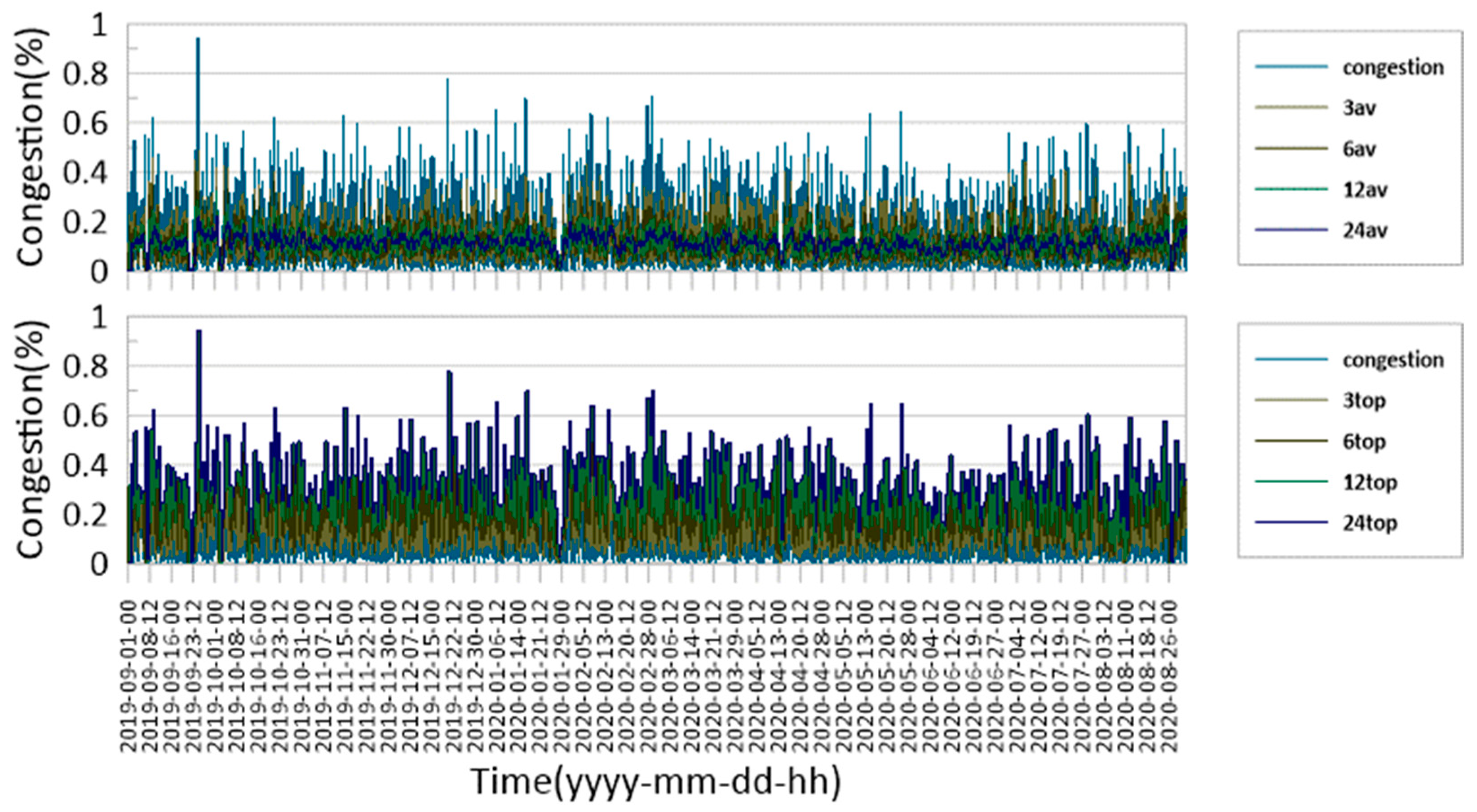
In addition, considering the characteristics of maritime traffic congestion, the average and maximum values for 3, 6, 12, and 24 days were selected as the features. Figure 5 illustrates the results of analyzing the average, maximum, and minimum maritime traffic congestion for 3, 6, 12, and 24 days.

4.4. Training and Experiment

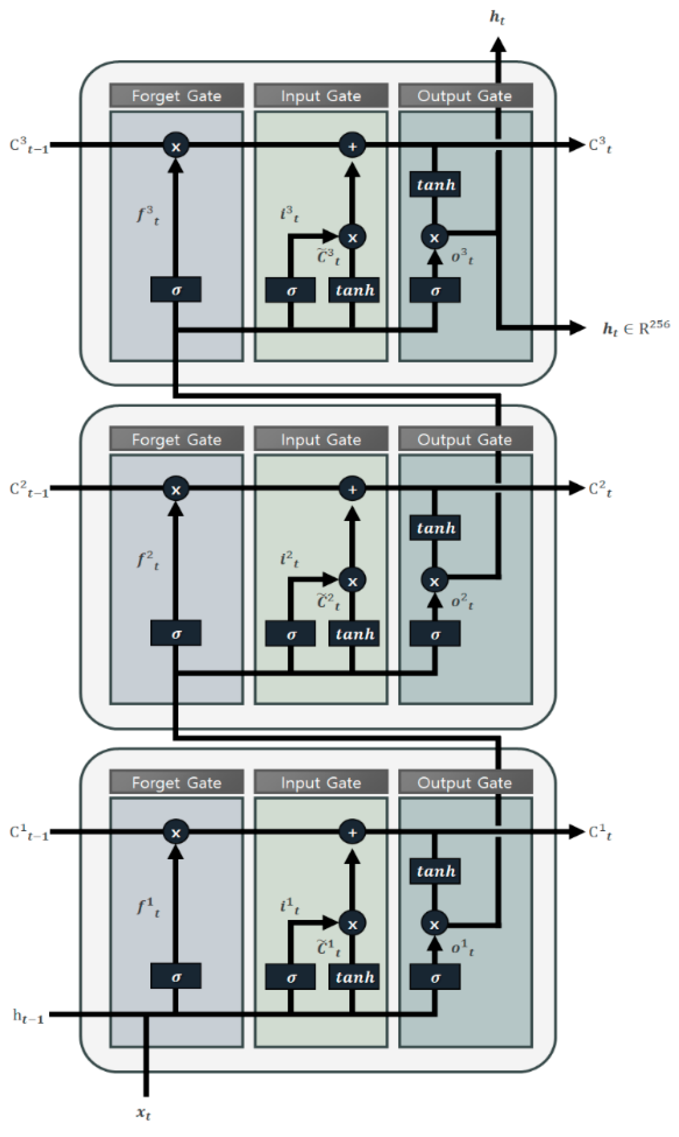
The training model was designed using LSTM considering that maritime traffic data are time-series data. Although LSTM has the drawbacks of requiring a long training time, consuming a large amount of memory, and being vulnerable to overfitting and sensitive to random weight initializations, it was chosen due to its ability to handle long-term dependencies and overcome the vanishing gradient problem commonly found in time series prediction tasks. The LSTM includes three gates: input, forget, and output; each gate determines the important information from the past and present input information via the sigmoid and hyperbolic tangent functions [37]. The LSTM was composed of three layers, and the hidden layer was set to 256 dimensions. The dimension of input layer changes depending on the scenario. Figure 6 illustrates the configuration of the LSTM in the developed algorithm while

Table 2. Hyperparameters for training.

Hyperparameters	Value
Batch Size	24
Dropout Rate	0.6
Epoch	500
Learning Rate	0.001
Time Step	24
Optimizer	Adam
Weight initializer	Glorot_uniform
Gradient clipping	Clip_by_value

summarizes the hyperparameters for training.

The ratio between the training and validation data for the model was set as 8:2. We conducted an evaluation by dividing the data into 7:3 for training and validation and compared the results with the previous 8:2 division. We did not observe significant differences in the trend of result. The normalized mean square error (NMSE) was used as the loss function. The mean square error (MSE) and NMSE are calculated using

$$\mathrm{MSE}\left(\mathrm{x}, \mathrm{y}\right)={\sum }_{\mathrm{i}}{\left({\mathrm{x}}_{\mathrm{i}}-{\mathrm{y}}_{\mathrm{i}}\right)}^2/n$$

(14)

$$\mathrm{NMSE}\left(\mathrm{x}, \mathrm{y}\right)=\mathrm{MSE}\left(\mathrm{x}, \mathrm{y}\right)/\mathrm{MSE}\left(\mathrm{x}, 0\right)=\Vert \mathrm{x}-\mathrm{y}{\Vert }_2^2/\Vert \mathrm{x}{\Vert }_2^2$$

(15)

A total of eight training scenarios were created by dividing the features into the trend and prediction.

Table 3. Configuration of training and experimental scenarios.

No.	Input		Output
	Trend	Prediction
(a)	Congestion	-	Congestion
(b)	Congestion Variance width/rate/Prob.	-
(c)	Congestion 3, 6, 12, 24 avg	-
(d)	Congestion 3, 6, 12, 24 max	-
(e)	Congestion	Num of ship Traffic Vol
(f)	Congestion Variance width/rate/Prob. 3, 6, 12, 24 avg 3, 6, 12, 24 max	Num of ship Traffic Vol
(g)	-	Congestion (B gate) Congestion (C gate)
(h)	Congestion Variance width/rate/Prob. 3, 6, 12, 24 avg 3, 6, 12, 24 max	Number of ships Traffic Volume Congestion (B gate) Congestion (C gate)

lists the training and experimental scenarios.

4.5. Experimental Result

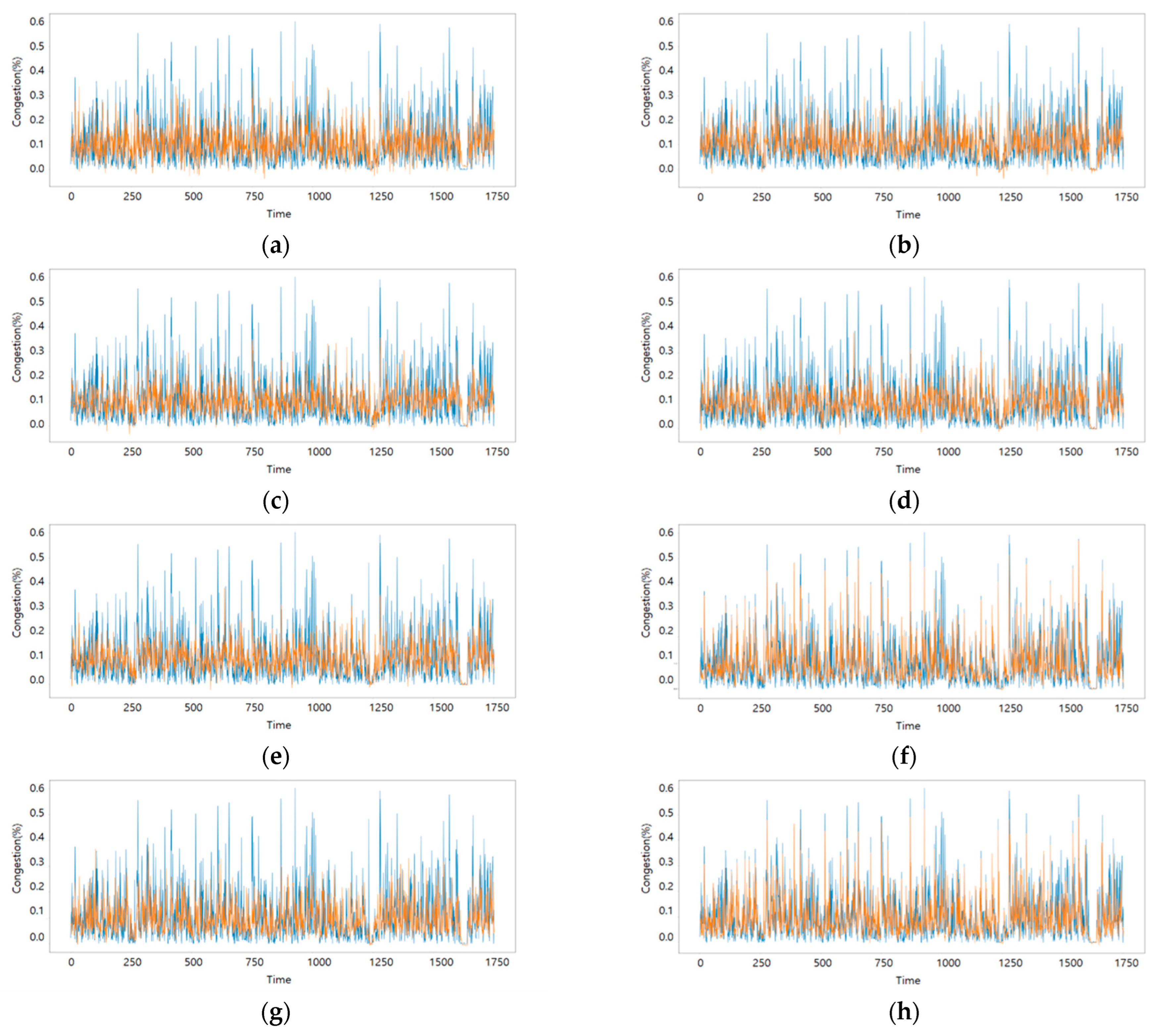
Based on model training and validation according to the scenario configurations, the valid loss was determined to be 0.2717 in scenario (a) using only congestion. However, in scenario (b) where the fluctuation range, fluctuation rate, and probability of varying within the fluctuation range were examined, the model performance improved to 0.2182.

Scenario (c) considered congestion and the average value of congestion on days 3, 6, 12, and 24 and scenario (d) considered the maximum value on days 3, 6, 12, and 24; they exhibited valid losses of 0.1490 and 0.1164, respectively. These values were higher than that of the previous two scenarios. Particularly, in the case of scenario (d), relatively high congestion was well predicted. Scenario (e) utilized congestion, the number of ships, and traffic volume, and had a valid loss of 0.2047. This suggested that the performance of the model improved, similar to scenario (b). When all the features were used except for the congestion of the other gate lines in scenario (f), the valid loss was 0.0842, which exhibited high model performance. When using the congestion of the other gate lines in scenario (g), the valid loss was 0.1520, which demonstrated that the performance of the model was further improved compared to scenarios (b) and (e). When all features were used in scenario (h), the valid loss was 0.0835, which was the highest model performance.

Figure 7 and

Table 4. Training and valid losses under each scenario.

No.	Training Loss	Valid Loss
(a)	0.2094	0.2717
(b)	0.1574	0.2182
(c)	0.1205	0.1490
(d)	0.0943	0.1164
(e)	0.1491	0.2047
(f)	0.0647	0.0842
(g)	0.1116	0.1520
(h)	0.0677	0.0835

depict the model training results for each scenario, where sky blue represents the validated data and orange indicates the predicted data.

5. Algorithm Validation

Algorithm validation was performed using additional data that had not been used in the training and validation processes for the model under scenario (h).

Table 5. Data for verifying the results of the model.

Train Data	Validate Data	Test Data
0.8	0.2
1 week		1 day
1 month		1 week
3 months		1 month
6 months		3 months

summarizes the data used for verifying the results of the model.

In the model training results, the valid loss was the lowest (0.0605) when using one-month data and the second lowest (0.0801) when using three-month data.

Table 6. Model training results according to the train/validate data length.

Train/Validate Data	Train Loss	Valid Loss
1 week	0.0514	0.1111
1 month	0.0367	0.0605
3 months	0.0570	0.0801
6 months	0.0744	0.1016

summarizes the model training results based on the train/validate data length.

A higher performance was observed as the size of the train/validate data and test data increased and when the model trained according to the train/validate data length was validated by changing the length of the test data. The performance was guaranteed to some extent when the data for more than a week were predicted using the data of at least three months.

Table 7. Model validation results according to the length of data.

Train/Valid Data	Test Data
	3 Months	1 Month	1 Week	1 Day
	NMSE
1 week	1.3919	1.4061	1.4141	1.4293
1 month	1.2895	1.3209	1.3663	1.4961
3 months	1.1746	1.2337	1.2543	1.3448
6 months	1.2150	1.2136	1.2552	1.5561
	RMSE
1 week	0.1133	0.1247	0.1229	0.1242
1 month	0.1100	0.1217	0.1186	0.1206
3 months	0.1041	0.1168	0.1151	0.1186
6 months	0.1058	0.1159	0.1154	0.1224
	MAE
1 week	0.0793	0.0882	0.0888	0.0979
1 month	0.0791	0.0871	0.0861	0.0950
3 months	0.0741	0.0844	0.0845	0.0853
6 months	0.0752	0.0826	0.0833	0.0848

and Figure 8 present the model validation results based on the data for the validated result length.

The results of this study were compared to those of a paper that predicts maritime traffic flow, although not in the exactly same field, using a model trained on 6-month data to predict 3-month data. The comparison showed an improvement in performance, with a decrease in RMSE from 0.942 to 1.342 and a decrease in MAE from 1.448 to 1.698.

Table 8. Comparison of results with other prediction model.

Performance Metrics	Proposed Method	Son et al. [17]
		CNN	LSTM	BDLSTM-CNN
RMSE	0.1058	0.2400	0.2100	0.2000
MAE	0.0752	0.2450	0.2250	0.2200

and Figure 9 are comparison of the results.

6. Conclusions

This study proposed a method of using data augmentation and LSTM to predict future maritime traffic conditions. Scenarios were established by combining various features, and model training and evaluation were performed. The results confirmed that the performance of the model improved as more features were applied. The maximum values for 3, 6, 12, and 24 days and the congestion of the gate lines around the analysis point showed a significant effect on performance. The algorithm validation results based on the length of train/validate data and test data indicate that a higher performance was observed with an increase in the size of data. The performance was guaranteed to some extent when data for more than a week were predicted by constructing the model using the data of at least three months.

The limitations of this study are as follows:

(1)

Maritime traffic congestion was predicted by applying the developed algorithm to a specific point in one port; therefore, it is necessary to perform evaluation for various points in several ports.

(2)

The congestion of nearby gate lines was used as a feature. This could decrease the accuracy of the algorithm if the influence of the nearby gate lines on the gate line to be predicted is insignificant based on the scenario.

Despite these limitations, the results of this study can be used to improve the performance of the situation recognition system of autonomous ships for identifying the current maritime traffic conditions and predicting the future maritime traffic conditions by identifying features for predicting maritime traffic conditions, constructing a model, and presenting the appropriate length of data for prediction. Further, they are expected to be used in maritime traffic condition recognition technology for coastal ships that navigate more complex sea routes compared to ships navigating the ocean. As a future study, we plan to evaluate algorithms developed for various ports and prepare countermeasures for cases where the influence of neighboring gate lines is small as a feature for predicting maritime traffic congestion. In addition, the performance of this algorithm will be validated by combining the situational awareness system of an autonomous ships with generation routes, collision avoidance, and returning routes of a coastal autonomous ships navigating complex sea areas.