Abstract
Human mobility influenced the spread of the COVID-19 virus, as revealed by the high spatiotemporal granularity location service data gathered from smart devices. We conducted time series clustering analysis to delineate the relationships between human mobility patterns (HMPs) and their social determinants in California (CA) using aggregated smart device tracking data from SafeGraph. We first identified four types of temporal patterns for five human mobility indicator changes by applying dynamic-time-warping self-organizing map clustering methods. We then performed an analysis of variance and linear discriminant analysis on the HMPs with 17 social, economic, and demographic variables. Asians, children under five, adults over 65, and individuals living below the poverty line were found to be among the top contributors to the HMPs, including the HMP with a significant increase in the median home dwelling time and the HMP with emerging weekly patterns in full-time and part-time work devices. Our findings show that the CA shelter-in-place policy had varying impacts on HMPs, with socially disadvantaged places showing less compliance. The HMPs may help practitioners to anticipate the efficacy of non-pharmaceutical interventions on cases and deaths in pandemics.
1. Introduction
The 2019 novel Corona Virus (COVID-19) spread is an ongoing global public health emergency and has caused a profound impact on medical services around the world. Many health systems have had to quickly adapt to new technologies and procedures to better diagnose and treat patients [1,2,3,4]. Non-pharmaceutical actions, such as physical distancing and sheltering-in-place, were regarded as critical and implemented by many governments, especially when vaccines or therapeutics were not available. Precise anonymized location data collected from geographic location services provided a useful method to reveal human mobility at its finest granularity and frequency and to study the efficacies of non-pharmaceutical interventions enforced by national or local governments. Therefore, many aggregated human mobility datasets are derived and used in such efforts due to advances in, nowadays, geographic location services. Buckee et al. [5] highlighted how those aggregated mobility datasets can help fight the spread of COVID-19 and shed light on understanding the effectiveness of large-scale governmental social distancing public interventions. Many recent studies, with the help of using aggregated human mobility indicators from various datasets, demonstrated the effects of actions on reducing mobility as either containing the spread or mitigating the impacts of COVID-19. Kraemer et al. [6] calculated mobility statistics using Baidu’s real-time travel data and found that the restrictions on mobility implemented in China successfully contained the spread and reduced the local transmission of COVID-19 among the cities of China at the start of 2020. Gatto et al. [7] reported that “the sequence of restrictions imposed on mobility and human-to-human interactions reduced transmission by 45%” (42–49% confidence interval) from 21 February to 25 March 2020, in Italy, by running a susceptible-exposed-infected-recovered (SEIR) transmission model under various simulation scenarios. Vokó and Pitter [8] identified the changing points of the country-specific social distance index curves in 28 European countries and showed how COVID-19 growth rates were reduced by increasing social distancing quartiles after those change points. Similarly, Sulyok and Walker [9] used Google’s aggregated county-based community mobility reports (CMR) and found noticeably negative correlations between CMR mobility changes and COVID-19 case incidence for prominent industrialized countries in Western Europe and North America. Hadjidemetriou et al. [10] showed that human mobility in the United Kingdom gradually decreased as lockdown measures were announced and stabilized at around 80% after lockdowns were imposed; initial control measures aiming at human mobility reduction had a direct impact on the number of COVID-19 related deaths in the UK through the use of Apple’s mobility trend reports based on requests for directions in Apple Map services categorized by walking and driving.
While leveraging the power of human mobility datasets in investigating the spread and impacts of COVID-19, researchers also noted the luxury nature of those multi-source mobility datasets (e.g., SafeGraph) and the high spatial and temporal variations of their variables. [11] For example, The U.S. Centers for Disease Control and Prevention (CDC) [12] reported different temporal trends of social mobility in New Orleans, LA, New York City, NY, San Francisco, CA, and Seattle, WA, following the imposition of stay-at-home orders in these cities from 26 February to 1 April 2020 using aggregated GPS data from the SafeGraph. Moreover, Hou et al. [13] claimed that such spatial heterogeneities of social distancing might even exist within a county in their work on utilizing the location-based metrics of foot traffic to businesses and consumer points of interest provided by SafeGraph to augment a stochastic SEIR model. Those factors of high spatial and temporal variations reflect how the temporal patterns of a human mobility variable are more detailed and, as such, more appropriate to describe human mobility changes in comparison with the summary statistics (i.e., means). Thus, more advanced methods than calculating the mean values of the variable are needed to discover the human mobility pattern (HMP) in an aggregated form of a certain region. Huang et al. [14] pioneered a work using a K-means time series clustering algorithm to distinguish different HMPs at the census block groups level using the variable of the median home dwelling time provided by SafeGraph. The three types of HMPs identified via their methods in the Metropolitan Atlanta area affirmed substantial intra-county spatial heterogeneities and pointed to the existence of extensive gaps in the effectiveness of social distancing measures between socially disadvantaged groups and others. Similar studies focused on the HMPs of other mobility variables as traveled distances and visitation rates, and also confirmed that the speed, depth, and duration of social distancing in the United States were heterogeneous [15].
Efforts to socially distance may be more burdensome for some socially disadvantaged communities than others, which would potentially exacerbate disparities in COVID-19-related health outcomes. Researchers, with the help of SafeGraph data, found that individuals in high-income neighborhoods increased their days at home substantially more than individuals in low-income neighborhoods and that residents of low-income neighborhoods were more likely to work outside the home compared to residents in higher-income neighborhoods [16]. These findings point out the fact that lower-income people have faced barriers in complying with state physical distancing policies. However, these analyses were based on the national average HMPs of people within different income quintiles and ignored both the geographical variations inside those income quantile groups and the impacts from other social, economic, and demographic (SED) variables. In addition, several studies have found correlations between compliance with human mobility restriction orders and several social characteristics of local populations. Chiou et al. [17], for example, found that the combination of “having both high income and high-speed Internet appears to be the biggest driver of propensity to stay at home” using data that tracks 20 million mobile devices and their movements during the first few months of the early pandemic. Huang et al. [18] concluded that the lower compliance with stay-at-home orders among low-income groups in the 12 most populated metropolitan statistical areas in the United States was likely due to the fact that these groups could not afford to comply with such orders. This research inspired us to develop intelligent HMP discovering methods to study these SED inequalities at finer geographical scales because they are likely to amplify existing health disparities and must be addressed to ensure the success of ongoing pandemic mitigation efforts.
In this study, we used a dynamic-time-warping self-organizing map (DTW-SOM) clustering algorithm to classify the HMPs in CA census block groups, which has been well tested in clustering time series with asynchronous patterns [19]. We would like to address and solve this asynchronous pattern issue using DTW-SOM, as it allows for small tolerance on time shifting for HMPs. For example, some places might be faster in response to the shelter-in-place orders by a few days than others [11], but if their HMPs are similar in shape, we would assume that these places had similar compliance with orders. We noted that different human mobility variables might present unique and even contrasting characteristics. Thus, we ran the DTW-SOM on five different human mobility variables from SafeGraph to identify the HMPs of each variable and to reveal the multifaceted nature of human mobility. Since the identified HMPs reflect individual behaviors under government orders and personal perspectives of disease prevalence and their choice or ability to comply with stay-at-home orders, we next further investigated their associations with SED status and inequities. A recent study quantitatively evaluated the impact of human mobility on the spread of COVID-19 from a spatiotemporal perspective using geographically weighted regression and revealed the spatiotemporal-varying quantitative relationships between COVID-19 transmission and human mobility [20]. However, disparities in human mobility are the results of SED determinants, but fewer evaluated the quantitative relationships between human mobility and SED status. In many existing qualitative studies, SED variables were used to stratify the population and to compare the average human mobility of each stratification [16]. To overcome such challenges, we first collected 17 SED variables from the 2014–2018 American Community Survey to explain HMPs, then performed the analysis of variance (ANOVA) to examine whether the SED differences among HMP groups were statistically significant, and lastly, performed linear discriminant analysis (LDA) on the HMP groups to examine the quantitatively discriminating ability of 17 SED variables by their potency indices. To eliminate the impacts from confounders, such as the different contents of social distancing orders by different local governments under different pandemic reaction stages, we focused our study on the early pandemic period of California until 2 October 2020, when a new shelter-in-place order was released and enforced.
2. Materials and Methods
We selected five human mobility indicators derived by SafeGraph: (1) median home-dwelling time; (2) the percentage of completely stay-at-home devices; (3) the percentage of frequently moving devices as would happen when, for example, making deliveries; (4) the percentage of stationary part-time (work) devices at locations other than at home; and (5) the percentage of stationary full-time (work) devices at locations other than home. They were calculated based on an aggregated anonymous mobile device by SafeGraph, which aggregated physical locations of non-identifiable individuals collected from third-party entities under licenses that complied with evolving laws regarding privacy to the census block group (CBG) level (Table 1). SafeGraph used the typical nighttime (i.e., from 6 p.m. in the evening to 7 a.m. the next morning) location over a 6-week period to assign “homes” to each of the participating devices. The initial assignments were made for squares measuring approximately 153 m on a side and then census block groups containing these squares. The daily median home dwelling time was calculated as the median number of minutes at home on a given day across all devices located in a given census block group. The percentage of devices completely staying at home was calculated by dividing the number of devices that did not leave their home squares located in a CBG with the number of devices seen during the same date range whose home was in that CBG. The full- and part-time work behavior devices were those that spent > 6 h and 3–6 h in places other than the designated “home” location from 8 a.m. to 6 p.m. each day. The mobile (delivery) behavior devices stopped for < 20 min at > 3 locations per day in some place other than the designated “home” location.

Table 1.
Social, economic, and demographic variables selected from the 2014–2018 American Community Survey.
We obtained these 5 indicators from 1 January 2019 to 3 October 2020 for the whole U.S. and extracted the devices located in CA for further analysis. The reason for choosing CA as our study location was due to the severe impact that the COVID-19 pandemic had on this area. This included state-implemented measures, such as lockdowns and gathering restrictions, to control the spread of the virus and to address the evolving situation. We excluded the census block groups (CBGs) in census tracts with “98” prefixes, which marked places of a large area with few or no residents, such as large parks or employment areas, and “99”, which denotes large bodies of water. The final dataset included 23,142 census block groups, and the daily numbers of tracked mobile devices ranged from 1.74–2.58 million in 2019 to 1.37–1.93 million in 2020. Given the total number of 39.78 million residents, based on the 2020 U.S. Census, these metrics meant that we were able to track 4.5–6.5% and 3.5–5% of the total population in California in 2019 and 2020, respectively. To avoid the seasonality of human mobility caused by climatic drivers, school terms, religious festivals, and national holidays [21], we subtracted the daily values of 2020 from the five variables by their daily values in 2019 so that a positive value would mean an increase in the variable and vice versa. To match the day of the week, we calculated the changes in these five metrics by subtracting their daily values in 2020 from the daily values in 2019 using a 1-day lag before 29 February 2020 and a 2-day lag thereafter (since 2020 was a leap year). This approach meant that we could compare similar days across the two years. This was important because the human mobility metrics reveal strong weekly patterns. For example, median home dwelling times regularly peaked on weekends. As a consequence, the HMPs represented the 2019–2020 patterns of changes of the five metrics.
We used time-series clustering methods to characterize temporal mobility patterns across geographic units [22]. We were able to produce HMP groups that were less sensitive to outliers and with lower clustering errors in our preliminary analyses using DTW-SOM: a self-organizing map clustering algorithm variant previously developed by our research group [19,21]. A self-organizing map is a type of unsupervised neural network with only two fully connected layers: an input layer and an output or mapping layer. This approach provides a competitive learning neural network since the weights in it have different meanings than in standard neural networks. Each weight on a connection in SOM represents the similarity between the connected mapping neuron and the input neuron. The SOM transforms the input space into a lower, typically two-dimensional gridded space that is effective for visualizing and exploring the properties of the input data. This method has been widely applied in time-series clustering [23,24]. In our dynamic time-warping DTW-SOM method, the similarity measure (i.e., DTW) optimally aligns interior patterns in the sequential data, both as the similarity measure and training guide of the neural network. DTW-SOM produces lower clustering errors and higher purity within each output neuron, especially when applied to time series input data than standard self-organizing maps.
We ran DTW-SOM on clustering each one of the 5 human mobility indicators using initial weights for the neurons calculated by principal component analysis (PCA) with a learning rate of 0.5. We chose 4 as the number of groups for each mobility indicator to balance the trade-off between clustering errors and interpretability. We monitored the clustering quantization errors of the output space and stopped the training progress when the errors converged (<0.001). At the end of the training of each mobility metric, DTW-SOM assigned the CBGs to one of the four neurons, whose weights represent HMPs of that mobility metric. For ease of later reference, we denoted the groups generated by (1) the median home-dwelling time as time-HMP-groups; (2) the percentage of completely stay-at-home devices as home-HMP-groups; (3) the percentage of delivery (work) devices as delivery-HMP-groups; (4) the percentage of part-time (work) devices as part-HMP-groups; and (5) the percentage of full-time (work) devices as full-HMP-groups. We also named the four groups under each metric using the order of their group means so that time-HMP-group one denoted the group with the smallest mean, which was generated by applying DTW-SOM on the median home-dwelling time variable and, similarly, time-HMP 4 represented the HMP (cluster center) of the time-HMP-group 4, which had the largest mean under the same metric. This nomenclature would allow us to more easily refer to various groups generated by different human mobility metrics and explain our hypothesis that HMPs offer fine-grained mobility profiles and, therefore, are superior to mean values in investigating the complex relations between human mobility and other socioeconomic and demographic factors.
We downloaded 17 social, economic, and demographic variables for all CBGs in California from the 2014 to 2018 American Community Survey (Table 1).
For each mobility indicator, we related the HMPs discovered by DTW-SOM to the 17 SED factors using two complementary approaches: one univariate and one multivariate. In the univariate approach, we used one-way ANOVA to quantify the variation in each SED factor across the 4 HMP groups. In the multivariate approach, we assigned the 4 HMP groups for each human mobility indicator into two groups, consisting of one group that had a typical HMP of interest versus the other group that did not, due to the following reasons: (1) The 4 HMPs of each mobility indicator discovered by DTW-SOM were not all equally representative. Some of them were much less populated than others (i.e., group 2 in the delivery behavior HMP groups only had 569 CBGs whereas the largest group 1 had 14,650 block groups); (2) Meanwhile, it would be very tedious to discriminate the differences between each two out of the groups. Thus, we decided to focus on the typical HMPs that we had the most interest in and dichotomized the groups according to whether they had that kind of HMP or not. For example, we had two groups that were derived based on the DTW-SOM results of the full-time work mobility indicator. One group contained CBGs showing an HMP of strong weekly patterns with periodic peaks during weekends, whereas the other one consisted of CBGs that did not show such an HMP. The detailed dichotomization schema is listed below:
- Full-time work behavior HMP groups (group 1 vs. others): HMP in group 1 showed lower values in 2020 than in 2019 (negative changes indicated by the centroid curve below the zero-baseline all the time), and the most apparent sharp decline took place right after the pandemic period started. Most importantly, strong weekly patterns with periodic peaks during weekends started to emerge with this HMP after the pandemic period started. We decided to group other HMP groups together because they ed no such HMP (group 2 showed a vaguely similar HMP but looked more closed compared to the rest of the groups), and we were interested to see what other SED variables contributed to the emergence of weekly patterns in such HMP.
- Part-time work behavior HMP groups (group 1 vs. others): The dichotomization schema and HMP profiles here were similar to what we conducted for full-time work behavior groups.
- Completely stay-at-home HMP groups (group 3, 4 vs. group 1, 2): HMPs in groups 3 and 4 here both have an obvious asymmetry peak pattern (even though at different levels), which increased at the beginning of the pandemic period and gradually decreased moving forward. In comparison, the other groups had either no or very modest HMP throughout the whole period.
- Home dwelling time HMP groups (group 3, 4 vs. group 1, 2): The dichotomization schema and HMP profiles here followed what we conducted for completely stay-at-home groups.
We then ran LDA to find the linear combinations of the SED factors that separated the two groups. The direction and magnitude of the LDA coefficients could be used to identify the factors that contribute the most, either positively or negatively, to distinguishing the two groups. While dichotomizing the HMP groups, we arbitrarily assigned 1 to the group with HMPs of interest and 0 to the other group since all the HMPs of interest indicated the tendency of the residents to stay at home longer, so that the LDA coefficients would always be positively correlated with the political compliance to the shelter-in-place order.
3. Results
3.1. HMPs of the 5 Human Mobility Indicators
We applied DTW-SOM on all five indicators independently using an output space of four neurons and identified four types of HMPs for each indicator using the cluster centers of the four groups (Figure 1 and Figures S1–S4). The California statewide median home dwelling times recorded with the white line in the top subplot of Figure 1 from 1 January to 13 March in 2020 are similar to those in 2019 (but for a small misalignment to match the day of the week and minimize the impacts from the observed variability in weekly patterns). However, during the period from 13 March 2020, when the national emergency state started, to 15 June 2020, when the CA statewide shelter-in-place order ended, we observed a sharp rise that gradually disappeared after 23 May 2020, when thousands of people protested against the shelter-in-place order in California. From 15 June to 2 October 2020, when California issued a new shelter-in-place order, we saw a modest increase in home-dwelling time relative to the same period in 2019. We also saw that a sharp decrease occurred prior to 19 March 2020, when California issued the first statewide shelter-in-place order, as residents performed more out-of-home activities to prepare to stay at home.
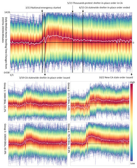
Figure 1.
CBG level CA 2019–2020 daily median home dwelling time changes of the whole state and the four time-HMP-groups.
The above statewide mean value curve informs us of a lot of temporal details concerning public responses and political compliance to the CA shelter-in-place order, however with such a highly populated and geographically versatile state as CA, we would expect more spatial variations of HMPs to be discovered, and the four subplots underneath Figure 1 showed the results of the four time-HMP-groups that were affirmed by our expectations. A large amount of CBGs, accounting for 15.2% of all the investigated CA CBGs in the time-HMP-group, 1 did not show any significant median home dwelling time increase with their cluster centroid line quite close to and slightly underneath the zero-baseline all the time. CBGs in time-HMP-group 2 featured fewer hours spent at home in early 2020 by having constant negative values before 13 March; however, these CBGs increased their hours at home rapidly after the shelter-in-place order. CBGs in time-HMP-group 3 and 4 spent similar amounts of time in hours at home in early 2020 before mid-March compared with the previous year and presented similar time-HMPs to the statewide time-HMP; thereafter, we still observed compelling differences among them. For example, time-HMP 4 still maintained momentous positive changes even after 15 June, but the positive changes disappeared in time-HMP 3 after 15 June. Moreover, the peak from 13 March to 15 June of time-HMP 3 is much closer to the peak of the statewide time-HMP and more moderate than the peak of time-HMP 4. The four types of time-HMPs informed us that only 43.9% CBGs (in group 3) had a similar time-HMP to the whole state, whereas over half of the CBGs in the state could not be described by the statewide time-HMP. Thus, using statewide time-HMP to describe all the CBGs could dismiss the facts that over 15% of CBGs did not change their median home dwelling times at all and over 40% of CBGs (time-HMP-group 2 and 4) experienced a momentous increase in their median home dwelling times after the end of the first shelter-in-place policy.
Similar geographical variations in HMPs were perceived on the other human mobility indicators as well. The percentage of completely stay-at-home devices is a human mobility indicator that is more correlated with the indicator of the median home dwelling time but potentially more relevant to the population in isolation or quarantine due to COVID-19, and we conducted similar clustering approaches on it. Its statewide home HMP showed a similar peak pattern but stayed below the zero-baseline before the national emergency started. Home-HMP 1, 3, and 4 showed that further different CBGs might have different levels of peaks. Although 17.6% of CBGs in group 4 showed a strong peak, the majority (31.8%) of CBGs in home-HMP-group 1 and 47.4% CBGs in home-HMP-group 3 did not respond as much. Meanwhile, a negligible portion of 3.2% CBGs in home-HMP-group 2 behaved completely differently than others, with the home-HMP 2 fluctuating fiercely around the zero-baseline (Figure S1). With these clustering results, we concluded that the population completely staying at home elevated significantly by over 96% CBGs (in home-HMP-group 1, 3, and 4) after the order, even though from a baseline much lower than the previous year was observed. Compared with the elevation in home-dwelling times observed in only around 85% of CBGs (in time-HMP-group 2, 3, and 4) after the order, we could claim stronger political compliance to the order by using the completely staying-at-home metric than the home-dwelling time metric. Moreover, unlike the momentous increases in the time-HMPs, which persisted in over 40% CBGs (in time-HMP-group 2 and 4) after the order, the momentous increases in home-HMPs persisted in only 17.6% CBGs (in home-HMP-group 4) after the order. This fact affirmed our initial attention that different indicators would reveal human mobility from different viewpoints.
Clustering results on both full-HMP-groups and part-HMP-groups also showed substantial geographical variations of HMPs. Statewide HMPs of both showed slender decreases in early 2020 before any social distancing order was enforced, and those decreases were slightly exacerbated when some weekly patterns emerged after mid-March. However, in some of the groups (e.g., full-HMP-group 1, part-HMP-group 1, and 4), a much stronger emergence of weekly patterns was observed after 13 March (Figures S2 and S3). Since we arbitrarily imposed a date misalignment to match the day of the week between 2019 and 2020, the weekly patterns were therefore minimized in calculating the changes, and we could see no weekly patterns in both HMPs before 13 March. Thus, we concluded that the emergence of the new weekly patterns, which manifested the considerable differences in both indicator changes between weekdays and weekends, was caused by the shelter-in-place order. These results further proved the spatial heterogeneities of both full-time HMPs and part-time HMPs. Finally, in comparison with all the other human mobility indicators, delivery-HMPs showed very little information about the whole state and all four subgroups. Those delivery-HMPs all concentrated on the zero-base line and stayed slightly below it. Delivery-HMP-group 2 and 4 revealed more temporal variations (Figure S4), but no obvious temporal shapes were observed. Nonetheless, due to the limited information provided by the HMPs for this indicator, we excluded it from our further analyses.
In Figure 1, different colors from the color bar were used to highlight the densities of the median home dwelling time change curves at the CBG level. The areas plotted in warmer colors represent a higher density of curves and vice versa. The black horizontal lines indicate the zero-change baseline for better visualization of positive or negative changes, and the white curves represent the centroids (HMPs) for the State of California or each time HMP group.
3.2. Geographical Locations of the HMPs
With the above evidence of the high geographical variations of the HMPs identified by DTW-SOM, we further investigated the geographical locations of these HMPs, in the active hope of associating the geographical distributions of these HMPs with their built-in environments and unique racial/ethnic distributions. Home-HMP 3 and 4 both showed strong peaks of increase during the shelter-in-place period and were mainly concentrated in the more developed areas (e.g., the bay area and the greater LA area, as shown in Figure 2). Other human mobility indicators with similar situations showed distinct compositions of HMPs between rural and urban areas. For example, full-HMP 1 and 2 and part-HMP 1 and 4 that showed a stronger emergence of weekly patterns were more concentrated in the developed and populated areas such as the bay area and the greater LA area (Figures S5–S8). The statewide spatial distributions of the HMPs sheds light on our hypothesized relationships between HMPs and local SED status.
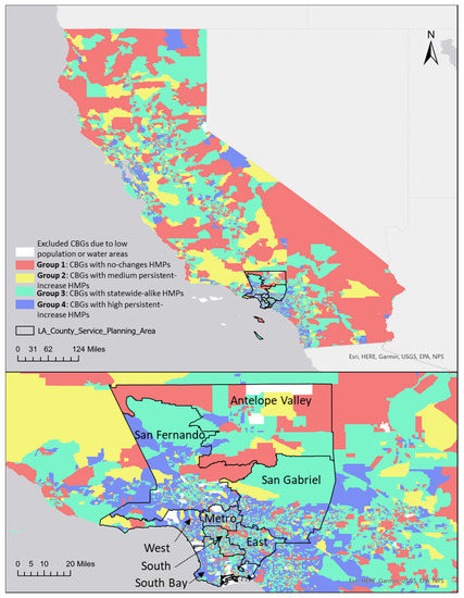
Figure 2.
Geographical locations of the CBGs in each median home dwelling time cluster of the whole CA state with an inset view of the SPAs of LA county.
An inset view focusing on LA county confirmed our hypothesis of the intra-county heterogeneity of HMPs, especially in a populous county as such. To better delineate the spatial distributions of the HMPs on a finer local scale taking the LA county as an example, we studied the prevalence of each type of HMP in each service planning area (SPA) of LA county. A service planning area, or SPA, is a specific geographic region within LA County with its unique racial/ethnic distribution for the purpose of developing more relevant public health and clinical services targeted to the specific health needs of the residents in the area. We calculated the prevalence of an HMP as the percentage of the total number of tracked devices grouped to the HMP (Figure 3). In Figure 3, Subplot A shows the percentages of the tracked devices of different median home dwelling times for HMP groups; Subplot B shows the percentages of tracked devices for different percentages of completely staying-at-home device HMP groups; Subplot C shows the percentages of tracked devices for different full-time work device HMP groups; Subplot D shows the percentages of tracked devices for different part-time work device HMP groups. We found that Metro SPA and South SPA had the lowest prevalence of HMPs with a strong peak of increase in the median home dwelling time (group 3 and group 4). It should be noted that Metro SPA and South SPA are the ones least likely to have sources of health care compared with other SPAs. Both had a larger proportion of adults reporting that they or their children were in fair or poor health, according to the 2018 LA County Health Survey [25]. The 2018 LA County Health Survey also brought to our attention that Metro SPA and South SPA both have the largest percentage of uninsured adults (South SPA: 16.6%; Metro SPA: 14.2%) with respect to other SPAs in the county. Meanwhile, San Fernando Valley SPA, San Gabriel SPA, and West SPA were among the top in terms of the prevalence of both full-time (group 1 and group 2) and part-time (group 1) HMPs showing the emergence of weekly patterns. CBGs in those areas tended to have larger negative changes during weekdays than during weekends, which means that those areas had a larger population with more awareness of the pandemic crisis and capabilities of transiting to work-from-home behavior under the compliance to the shelter-in-place order of the county. The 2018 LA County Health Survey told us that those SPAs were among the top in obtaining a flu vaccination in the past year (West SPA: 53.4% at rank 1; San Gabriel SPA: 49.3% at rank 3; San Fernando Valley SPA: 45.6% at rank 5), and those SPAs had the lowest percentage of households with reported food insecurity issues (West SPA: 12.4% at rank 1; San Gabriel SPA: 14.7% at rank 2; San Fernando Valley SPA: 15.6% at rank 3). Human mobility changes during the initial phases of the pandemic in the whole of the USA were found to be associated with conventional health behaviors (e.g., particularly less obesity and greater physical activity) and counties with healthier behaviors had a greater reduction in movement outside the home [26]. The distinguishing compositions of HMPs in each SPA and their associations with self-reported health conditions, insurance status, and vaccination behaviors upheld such national-wide conclusions at a much finer local scale.
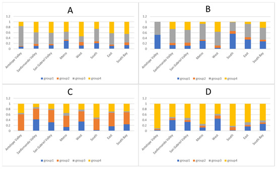
Figure 3.
Percentages of tracked devices of different HMP groups in SPAs of LA county (subfigures explained in Section 3.2).
3.3. Social Determinants of the HMPs
The geographical distributions of HMPs show big differences both statewide and among the SPAs (Figure 3), which means that people in places with different social factors reacted differently to the pandemic crisis and governmental orders along with it. To further investigate the statistical significance of the socioeconomic and demographic differences among the DTW-SOM groups, we selected 17 SED variables and tested their differences using ANOVA. The ANOVA test results reported in Table 2 demonstrate that the group means of all 17 SED variables are significantly different across the mobility groups for each of the human mobility indicators. Full descriptions of the SED variables’ abbreviations can be found in Table 3. Given that all the F-values (calculated by the ratio of between-groups variance over within-group variance) were significantly large (critical F-value is 3.78 and only the F-value lower than it is from the percentage of female in part-time work groups) and statistically significant (all p-values were smaller than 0.01), we conclude that almost all the SED variables have variability between the group means larger than the variability within the groups of each human mobility indicator and therefore that the CBGs with different HMPs have different SED characteristics. For example, we can see a large F-value (2890.76) of median income in stay-at-home mobility groups, which means that people with different stay-at-home HMPs have significantly different incomes. To further understand whether each type of HMP is positively or negatively associated with those SED factors, we conducted an LDA analysis in Table 3.
Table 2.
ANOVA test results for the socioeconomic and demographic variables and the five social mobility groups 1.
Table 3.
LDA analyses of the dichotomized social mobility groups using social-economic and demographic variables.
Table 3 lists the coefficients of the SED variables from LDA. A median household income and the median value of owner-occupied units were re-scaled to a range of 0–1 prior to LDA so that their coefficient scales would be comparable with other variables that were naturally defined as percentages within the range of 0–1. The LDA achieved good performances in terms of prediction accuracies ranging from 76.47% to 79.62%. The most contributable (either positively or negatively) SED variables are highlighted in Table 2. The percentage of the Asian population was found in the top-3 positively contributable for all four dichotomized HMP groups which favor both the HMP with a strong peak of increase in median home dwelling time and the HMP with the emergence of weekly patterns in full-time and part-time work devices. Both HMPs indicate that the residents in the CBGs belonged to those HMP groups who would have a tendency to stay at home longer. In contrast, we found the coefficient directions of the percentage of the over-65 male population to be totally opposite and have top-three loadings on all LDA equations for discriminating the HMPs. Moreover, median income was also found to be in the top-3 negatively contributable factors for most groups (except the stay-at-home behavior group). On the other hand, social impacts on HMPs from the percentage below the poverty line are among the negative top-3 variables for all HMP groups except for the part-time behavior device group (even though not top-3 but still highly negatively contributable). We also noted that the percentage of the under-5 population had top-3 negative impacts on the stay-at-home behavior HMP group but top-3 positive impacts on all other HMP groups.
4. Discussion
Human mobility changed during the COVID-19 pandemic because of various factors, including lockdowns, remote work, and increased concerns. The whole workflow and the results of this study shed light on the relationships between the geographic distributions of SED characteristics and the HMPs so that researchers could more accurately model the epidemiology of the virus and the impact of potential policy interventions to help identify the most effective non-pharmaceutical actions. Studying the disparities in HMPs due to SED characteristics is of great significance as it can help policymakers better understand why certain communities may have been more or less compliant with shelter-in-place orders. This understanding can then be used to develop targeted interventions and communication strategies that address the specific barriers to compliance within certain communities. Additionally, studying compliance disparities can help identify and address potential inequities in the enforcement of such orders, ensuring that all communities are treated fairly and equitably. Furthermore, understanding the SED factors that influence compliance with shelter-in-place orders can also inform future pandemic response efforts, helping to ensure that measures are designed in a way that maximizes compliance while minimizing negative impacts on communities. Overall, this study is essential for improving the effectiveness and equity of pandemic response efforts.
This study investigated the human mobility patterns at the CBG level proxied by five selected human mobility indicators and discovered two iconic HMPs and their top important social determinants (either positively or negatively). The 2 HMPs are the HMP with a strong asymmetry peak tailing to right in the indicators of median home dwelling time and completely stay-at-home devices and the HMP with the emergence of strong weekly patterns after a sharp decrease in values in the indicators of full-time and part-time work behavior devices. Both HMPs tend to favor better political compliance to shelter-in-place orders and provide a greater temporal context than pure value changes over time. For example, using the pure value changes of group 1 and group 3 in Figure 1 would totally dedifferentiate the two groups from each other since both groups have similar beginning values and ending values, even though group 3 has the HMP with a strong asymmetry peak whereas group 1 does not.
The fine spatial granularity at the CBG level to discover the HMPs is very important since considerable variations in HMPs were observed in CBGs within Los Angeles (Figure 2 and Figures S5–S8), which may have been obscured in a county-level analysis. For example, within LA county, many groups showed different proportions among SPAs. Many existing COVID-19 epidemiology models used global contact rates to model the transmission rates [27,28,29]. This study provided a base for delineating the spatial variability in HMPs and offered the opportunity to model COVID-19 at a finer spatial granularity with spatially varying transmission rates controlled by spatially varying HMPs.
This study also explored the roles of social determinants of SED factors for HMPs under COVID-19. Even though there were many existing studies on SED disparities of HMPs which confirmed that places with higher social deprivation scores experienced reduced mobility at lower rates and, therefore, a greater growth in COVID-19 cases and deaths [30], our study is the first to identify HMPs solely based on their temporal shapes compared to other methods that use the average HMPs of stratified SED groups. There are two inherent defects to using average HMPs of stratified SED groups: (1) The analysis is bounded to a certain SED variable (e.g., median income or social deprivation scores) and neglects the impacts that form other SED variables. (2) There are still spatial variations in terms of temporal shapes within each SED group which would be under-represented using the average values.
We examined the importance and directions of 17 SED factors on the changes in four selected human mobility indicators, and the results implied the different compliance to governmental non-pharma interventions (e.g., shelter-in-place order by the CA government) by different communities. For example, we speculate that the socially disadvantaged communities with a higher percentage of the population in poverty and lower incomes would most likely have less compliance with the shelter-in-place order. Meanwhile, both identified HMPs would be observed less in the older communities. Moreover, the percentage of the under-5 population would largely increase the chance of having an HMP peak in the median home dwelling time indicator but not the complete stay-at-home indicator. This contradictory fact emphasizes the necessity of investigating multiple indicators to obtain a better understanding of the whole picture of human mobility changes during the crisis.
We chose CA as our study area to remove the impacts of the time inconsistency of non-pharmaceutical interventions by different government agencies. However, the proposed framework could be expanded from only CA block groups to all national block groups in the future, and it laid out the foundation for studying the impacts of the social determinant variables on health outcomes (i.e., COVID-19 confirmed cases or COVID-19-related deaths) through impacts on social behaviors in the future. The DTW-SOM algorithm is currently publicly available through the Python library “dtwsom”.
Since this study is based on real-time GPS pings, it has the potential limitation of data reliability from the location services. For example, some outlier low median home-dwelling time values were observed on 25 February 2020 (Tuesday), which is neither a national holiday nor a day with any known big public events, elucidating the potential risks from either issue in location services or changes in GPS data processing protocols. This was also confirmed as a data artifact by SafeGraph on 2 March 2020. We ended up with the solution of imputing abnormal data using a median filter. Additionally, cell phone locations do not always correspond to the location of the user, as there may be instances where the device is not in possession of the owner. Future work needs to be focused on methodologies of preprocessing and aggregating the device-level tracking data and the generation of more informative human mobility indicators.
Supplementary Materials
The following supporting information can be downloaded at: https://www.mdpi.com/article/10.3390/app13042440/s1. Figure S1. Heat map of CA statewide daily percentage of completely at home device changes and the 4 DTW-SOM groups.; Figure S2. Heat map of CA statewide daily percentage of full-time worker behavior device changes and the 4 DTW-SOM groups. Figure S3. Heat map of CA statewide daily percentage of part-time worker behavior device changes and the 4 DTW-SOM groups. Figure S4. Heat map of CA statewide daily percentage of delivery worker behavior device changes and the 4 DTW-SOM groups. Figure S5. Geographical locations of the CBGs in each completely staying at home groups of the whole CA state with inset view of the SPAs of LA county. Figure S6. Geographical locations of the CBGs in each full-time work behavior device groups of the whole CA state with inset view of the SPAs of LA county. Figure S7. Geographical locations of the CBGs in each part-time work behavior device groups of the whole CA state with inset view of the SPAs of LA county. Figure S8. Geographical locations of the CBGs in each delivery work behavior device groups of the whole CA state with inset view of the SPAs of LA county.
Author Contributions
Conceptualization, K.L., E.G. and S.P.E.; methodology, K.L.; software, K.L.; validation, F.D.G., Z.C. and J.P.W.; formal analysis, K.L.; resources, J.P.W.; data curation, K.L.; writing—original draft preparation, K.L.; writing—review and editing, K.L., J.P.W. and S.P.E.; visualization, K.L.; supervision, F.D.G. and J.P.W.; project administration, E.G., funding acquisition, E.G. and K.L. All authors have read and agreed to the published version of the manuscript.
Funding
The author(s) disclosed a receipt of the following financial support for the research, authorship, and/or publication of this article: This research was supported by the National Institute of Environmental Health Sciences (grant #s P30ES007048 and P30ES007048-25S1), the Hastings Foundation, Taylor Geospatial Institute (grant# PROJ-000321), and by the Keck School of Medicine of USC COVID-19 Research Fund through a generous gift from the W.M. Keck Foundation.
Institutional Review Board Statement
Not applicable.
Informed Consent Statement
Not applicable.
Data Availability Statement
The data that support the findings of this study are available on request from the corresponding author, K.L.
Conflicts of Interest
The authors declare no conflict of interest.
References
- Plaza-Ruiz, S.; Barbosa-Liz, D.; Agudelo-Suárez, A. Impact of COVID-19 on the future career plans of dentists. Dent. Med Probl. 2022, 59, 155–165. [Google Scholar] [CrossRef] [PubMed]
- Flores-Quispe, B.M.; Ruiz-Reyes, R.A.; León-Manco, R.A.; Agudelo-Suárez, A. Preventive measures for COVID-19 among dental students and dentists during the mandatory social isolation in Latin America and the Caribbean in 2020. Dent. Med Probl. 2022, 59, 5–11. [Google Scholar] [CrossRef] [PubMed]
- Lewandowska, M.; Partyka, M.; Romanowska, P.; Saczuk, K.; Lukomska-Szymanska, M.M. Impact of the COVID-19 pandemic on the dental service: A narrative review. Dent. Med Probl. 2021, 58, 539–544. [Google Scholar] [CrossRef] [PubMed]
- Duś-Ilnicka, I.; Krala, E.; Cholewińska, P.; Radwan-Oczko, M. The Use of Saliva as a Biosample in the Light of COVID-19. Diagnostics 2021, 11, 1769. [Google Scholar] [CrossRef]
- Buckee, C.O.; Balsari, S.; Chan, J.; Crosas, M.; Dominici, F.; Gasser, U.; Grad, Y.H.; Grenfell, B.; Halloran, M.E.; Kraemer, M.U.G.; et al. Aggregated mobility data could help fight COVID-19. Science 2020, 368, 145–146. [Google Scholar] [CrossRef]
- Kraemer, M.U.G.; Yang, C.-H.; Gutierrez, B.; Wu, C.-H.; Klein, B.; Pigott, D.M.; Open COVID-19 Data Working Group; du Plessis, L.; Faria, N.R.; Li, R.; et al. The effect of human mobility and control measures on the COVID-19 epidemic in China. Science 2020, 368, 493–497. [Google Scholar] [CrossRef]
- Gatto, M.; Bertuzzo, E.; Mari, L.; Miccoli, S.; Carraro, L.; Casagrandi, R.; Rinaldo, A. Spread and dynamics of the COVID-19 epidemic in Italy: Effects of emergency containment measures. Proc. Natl. Acad. Sci. USA 2020, 117, 10484–10491. [Google Scholar] [CrossRef]
- Vokó, Z.; Pitter, J.G. The effect of social distance measures on COVID-19 epidemics in Europe: An interrupted time series analysis. Geroscience 2020, 42, 1075–1082. [Google Scholar] [CrossRef]
- Sulyok, M.; Walker, M. Community movement and COVID-19: A global study using Google’s Community Mobility Reports. Epidemiology Infect. 2020, 148, e284. [Google Scholar] [CrossRef]
- Hadjidemetriou, G.M.; Sasidharan, M.; Kouyialis, G.; Parlikad, A.K. The impact of government measures and human mobility trend on COVID-19 related deaths in the UK. Transp. Res. Interdiscip. Perspect. 2020, 6, 100167. [Google Scholar] [CrossRef]
- Huang, X.; Li, Z.; Jiang, Y.; Ye, X.; Deng, C.; Zhang, J.; Li, X. The characteristics of multi-source mobility datasets and how they reveal the luxury nature of social distancing in the U.S. during the COVID-19 pandemic. Int. J. Digit. Earth 2021, 14, 424–442. [Google Scholar] [CrossRef]
- Lasry, A.; Kidder, D.; Hast, M.; Poovey, J.; Sunshine, G.; Winglee, K.; Zviedrite, N.; Ahmed, F.; Ethier, K.A.; Clodfelter, C.; et al. Timing of Community Mitigation and Changes in Reported COVID-19 and Community Mobility—Four U.S. Metropolitan Areas, 26 February–1 April 2020. MMWR. Morb. Mortal. Wkly. Rep. 2020, 69, 451–457. [Google Scholar] [CrossRef]
- Hou, X.; Gao, S.; Li, Q.; Kang, Y.; Chen, N.; Chen, K.; Rao, J.; Ellenberg, J.S.; Patz, J.A. Intracounty modeling of COVID-19 infection with human mobility: Assessing spatial heterogeneity with business traffic, age, and race. Proc. Natl. Acad. Sci. USA 2021, 118, e2020524118. [Google Scholar] [CrossRef] [PubMed]
- Huang, X.; Li, Z.; Lu, J.; Wang, S.; Wei, H.; Chen, B. Time-Series Clustering for Home Dwell Time During COVID-19: What Can We Learn from It? ISPRS Int. J. Geo-Information 2020, 9, 675. [Google Scholar] [CrossRef]
- Garnier, R.; Benetka, J.R.; Kraemer, J.; Bansal, S. Socioeconomic Disparities in Social Distancing During the COVID-19 Pandemic in the United States: Observational Study. J. Med Internet Res. 2021, 23, e24591. [Google Scholar] [CrossRef]
- Jay, J.; Bor, J.; Nsoesie, E.O.; Lipson, S.K.; Jones, D.K.; Galea, S.; Raifman, J. Neighbourhood income and physical distancing during the COVID-19 pandemic in the United States. Nat. Hum. Behav. 2020, 4, 1294–1302. [Google Scholar] [CrossRef]
- Chiou, L.; Tucker, C. Social Distancing, Internet Access and Inequality; National Bureau of Economic Research Working Paper Series No. 26982; National Bureau of Economic Research: Cambridge, MA, USA, 2020. [Google Scholar] [CrossRef]
- Huang, X.; Lu, J.; Gao, S.; Wang, S.; Liu, Z.; Wei, H. Staying at Home Is a Privilege: Evidence from Fine-Grained Mobile Phone Location Data in the United States during the COVID-19 Pandemic. Ann. Assoc. Am. Geogr. 2021, 112, 286–305. [Google Scholar] [CrossRef]
- Li, K.; Sward, K.; Deng, H.; Morrison, J.; Habre, R.; Franklin, M.; Chiang, Y.-Y.; Ambite, J.L.; Wilson, J.P.; Eckel, S.P. Using dynamic time warping self-organizing maps to characterize diurnal patterns in environmental exposures. Sci. Rep. 2021, 11, 24052. [Google Scholar] [CrossRef] [PubMed]
- Lai, S.; Sorichetta, A.; Steele, J.; Ruktanonchai, C.W.; Cunningham, A.D.; Rogers, G.; Koper, P.; Woods, D.; Bondarenko, M.; Ruktanonchai, N.W.; et al. Global holiday datasets for understanding seasonal human mobility and population dynamics. Sci. Data 2022, 9, 17. [Google Scholar] [CrossRef]
- Chen, Y.X.; Chen, M.; Huang, B.; Wu, C.; Shi, W.J. Modeling the Spatiotemporal Association Between COVID-19 Transmission and Population Mobility Using Geographically and Temporally Weighted Regression. Geohealth 2021, 5, e2021GH000402. [Google Scholar] [CrossRef]
- Aghabozorgi, S.; Shirkhorshidi, A.S.; Wah, T.Y. Time-series clustering—A decade review. Inf. Syst. 2015, 53, 16–38. [Google Scholar] [CrossRef]
- Ritter, H.; Kohonen, T. Self-organizing semantic maps. Biol. Cybern. 1989, 61, 241–254. [Google Scholar] [CrossRef]
- Cherif, A.; Cardot, H.; Boné, R. SOM time series clustering and prediction with recurrent neural networks. Neurocomputing 2011, 74, 1936–1944. [Google Scholar] [CrossRef]
- Los Angeles County Department of Public Health. 2018 LA County Health Survey. Los Angeles, CA. Available online: https://www.publichealth.lacounty.gov/ha/hasurveyintro.htm (accessed on 31 July 2022).
- Bourassa, K.J.; Sbarra, D.A.; Caspi, A.; Moffitt, T.E. Social Distancing as a Health Behavior: County-Level Movement in the United States During the COVID-19 Pandemic Is Associated with Conventional Health Behaviors. Ann. Behav. Med. 2020, 54, 548–556. [Google Scholar] [CrossRef] [PubMed]
- Robles, B.; Thomas, C.S.; Lai, E.S.; Kuo, T. A Geospatial Analysis of Health, Mental Health, and Stressful Community Contexts in Los Angeles County. Prev. Chronic Dis. 2019, 16, E150. [Google Scholar] [CrossRef] [PubMed]
- Lai, S.; Ruktanonchai, N.W.; Zhou, L.; Prosper, O.; Luo, W.; Floyd, J.R.; Wesolowski, A.; Santillana, M.; Zhang, C.; Du, X.; et al. Effect of non-pharmaceutical interventions to contain COVID-19 in China. Nature 2020, 585, 410–413. [Google Scholar] [CrossRef]
- Weissman, G.E.; Crane-Droesch, A.; Chivers, C.; Luong, T.; Hanish, A.; Levy, M.Z.; Lubken, J.; Becker, M.; Draugelis, M.E.; Anesi, G.L.; et al. Locally Informed Simulation to Predict Hospital Capacity Needs During the COVID-19 Pandemic. Ann. Intern. Med. 2020, 173, 21–28. [Google Scholar] [CrossRef]
- Ossimetha, A.; Ossimetha, A.; Kosar, C.M.; Rahman, M. Socioeconomic Disparities in Community Mobility Reduction and COVID-19 Growth. Mayo Clin. Proc. 2021, 96, 78–85. [Google Scholar] [CrossRef]
Disclaimer/Publisher’s Note: The statements, opinions and data contained in all publications are solely those of the individual author(s) and contributor(s) and not of MDPI and/or the editor(s). MDPI and/or the editor(s) disclaim responsibility for any injury to people or property resulting from any ideas, methods, instructions or products referred to in the content. |
© 2023 by the authors. Licensee MDPI, Basel, Switzerland. This article is an open access article distributed under the terms and conditions of the Creative Commons Attribution (CC BY) license (https://creativecommons.org/licenses/by/4.0/).