Simulation-Based Analysis of the Effect of New Immersion Freezing Equipment on the Freezing Speed

Abstract

Modeling software was used to improve the efficiency of existing immersion freezing equipment. The concept of adding a rotating hopper device was proposed to make pork rotate with the rotating hopper in a flowing refrigerant carrier to achieve the effect of shortening the freezing time. In order to make up for the shortcomings of time-consuming processes and the limited information obtained from the measurement of the central temperature of pork, this paper establishes a mathematical model of the pre-freezing process using computational fluid dynamics (CFD) software to simulate the three-dimensional unsteady state of the pork. The simulation results show that when the rotating hopper is stationary, the refrigerant circulation flow shortens the freezing speed by 490 s compared to the freezing speed in the stationary state of the refrigerant carrier, and the freezing time efficiency is improved by 9.5%. When the refrigerant carrier flow rate v = 0 m/s and when the hopper speed r = 2 rad/s, the central temperature of pork drops rapidly from 26 °C to −15 °C in 0~1250 s, the decline leveled off at 1250–2310 s, and finally dropped to −18 °C, requiring a total of 5410 s. The freezing time of the immersion and freezing equipment was reduced by 2830 s after the addition of the rotating device, improving efficiency by nearly 55%. When the rotation speed r is increased from 2 rad/s to 4 rad/s, the freezing time is shortened by 1290 s and the freezing efficiency is increased by nearly 53%. The addition of the rotating device will make the pork freezing effect more uniform.

1. Introduction

Immersion freezing accelerates the freezing process by using liquid refrigerant. The use of liquid as a heat transfer medium with a high heat transfer coefficient is the main advantage of this freezing method [1]. Pork was frozen using liquid nitrogen, and a mathematical model simulating different freezing rates on the surface of frozen objects was solved by means of finite element analysis. The model fits the experimental data perfectly and predicts the local freezing rate at different locations in the pork tissue [2]. According to Liang’s investigation into the impact of impregnated freezing on the quality of lychee freezing, impregnated freezing increased the fruit’s overall quality and shelf life while increasing the freezing rate to 10 times that of air-cooled freezing [3]. Galetto compared freezing strawberries in a refrigerator at −26 °C to freezing strawberries by immersing them in a 30% CaCl₂ solution (−20 °C) for freezing [4]. Similarly, strawberry samples were cooled to −10 °C and freezing by immersion took only 30 min, compared to 75 min for freezing in a refrigerator. With the immersion freezing technique, the food is frozen in contact with a safe, non-toxic, low-temperature aqueous solution that has a freezing point below 0 °C, a process which is great deal faster than conventional freezing techniques [5].

Immersion freezing technology is divided into direct impregnation freezing technology and indirect impregnation freezing technology. Direct impregnation freezing not only needs to consider the heat transfer between food products and refrigerants, but also needs to consider the mass transfer between food products and refrigerants. Conversely, the same is not true for indirect impregnation freezing. With indirect impregnation freezing, the food must firstly be packaged in plastic for sterilization, and then the plastic package can be put into the refrigerant for freezing. Compared with the direct impregnation freezing technology, the indirect impregnation freezing technology is slower in freezing speed than the direct impregnation technology, but the advantage of the indirect impregnation technology is that it does not need to consider the material exchange between the refrigerant carrier and the frozen object, which improves the selectivity of the refrigerant carrier, improves the safety of the food, and the cost performance is significantly higher than the direct impregnation technology. Thus the majority of industrial impregnation production now uses indirect impregnation freezing technology to avoid the phenomena of heat and mass transfers between products and the refrigerant carrier.

The center temperature of frozen products must be below −18 °C, according to the international food freezing chain guideline [6]. The electric thermocouple measurement technique is typically used to determine the interior temperature of foods when they are frozen, but it is expensive, time-consuming, and has many restrictions. Computational fluid dynamics (CFD) may be an effective way to address this issue.

Serenity [7] studied the effects of various dry ice blasting velocities (0.10, 0.15, 0.20, 0.25, 0.30, 0.40, 0.50 m/s), radii of the blast inlet (18, 20, 23, 25, 30 mm), and dry ice blasting durations (0.10, 0.15, 0.20, 0.25, 0.30, 0.40, 0.50 s) on the strawberry quick-freezing process in the quick-freezing room. The effect of varying the dry ice volume fraction in the model at speeds of 0.20 and 0.30 m/s accelerated the ability of strawberries freeze rapidly. For the freezing of pork cubes in cylindrical tanks, Yan [8] created a transient variable physical heat transfer mathematical model. The simulation results at various stages of the freezing process showed the temperature distribution and the condition of the pork at each step of freezing. In order to model irregular shrimp and forecast the freezing period of the symmetrical section of shrimp at 15, 50, and 100 mm from the bottom of the freezer layer, respectively, Tang [9] employed the finite difference element approach. In a 3D non-stationary numerical simulation, Yao [10] used Fluent 6.3 software to simulate the temperature field of the carrot pre-freezing process and the dynamic propulsion process at the frozen phase change interface. Wang [11] created a three-dimensional numerical model for blast freezing of short cylindrical mashed potatoes. He then performed three-dimensional unsteady state numerical simulations and examined the freezing process of potatoes by combining the flow field and the temperature field at various points. He found that as the wind speed increased, the freezing time decreased and the temperature difference between the inside and outside of the mashed potatoes increased. The freezing process and freezing time of the thermal center and boundary layer of flat silver carp meat were predicted by Liu [12] using the finite difference method, showing that by combining the prediction model of thermal physical parameters and numerical simulation, the established model has high fitting accuracy and can simulate the freezing process of silver carp meat with various t values. Tian [13] simulated the freezing of a NaCl storage plate using numerical methods at various temperatures and then experimentally confirmed the simulation’s accuracy. Ni [14] used abalone as the research subject to investigate immersion fast freezing. He developed a three-dimensional unsteady numerical calculation model of abalone based on computational fluid dynamics, chose a freezing calculation model, established a polynomial calculation method for the thermal properties of abalone, improved the accuracy of the freezing process of abalone, the temperature distribution state of frozen abalone is obtained. Chen [15] predicted the temperature and humidity fields of the freezing process of eggplant using numerical simulations. In order to simulate temperature variations and moisture migration during the freezing process of eggplant at various freezing rates and thicknesses, the model took into account the porous structure inside the eggplant. In order to calculate the time needed to freeze fish and beef, Sepahvandi [16] created geometric models for fish and beef and a two-dimensional CFD model to mimic the cooling process in the refrigerator’s freezing channel.

In this paper, CFD software is used to simulate and analyze the effects of different speeds of the hopper and different liquid velocities on the freezing effect and speed of frozen objects. Based on the simulation results, an innovative improvement is proposed for the immersion refrigeration equipment. By adding a rotary device, the simulation requirements have been met. This equipment can be used by the food industry to quickly freeze perishable foods. This equipment is limited to specific types of frozen objects. In this paper, pork is the only product used for simulation analysis and description. The new freezing method and numerical simulation method proposed in this paper provide some theoretical guidance for the in-depth study of food immersion freezing technology and the guidance of actual production.

2. Materials and Methods

2.1. Experimental Setup

A freezing bin, a circulating water pump, a freezing unit, and a circulating water line are the components of the current immersion freezing apparatus. The downside of the current technology is that while products can be quickly frozen, they cannot be frozen evenly. In order to achieve a more uniform freezing effect, this paper suggests a novel idea: adding a rotating mechanism to the existing water circulation ultra-low temperature impregnation freezing equipment. This will allow the freezing bin to rotate at a constant speed while being circulated with the refrigerant.

Figure 1 and Figure 2 illustrate the equipment. This equipment primarily consists of a rotating hopper, a freezing unit, a freezing bin, and a liquid circulation pump. To achieve the quickest pre-cooling stage, the condenser tube is near to the freezer bin’s stainless steel outside wall. The freezing bin must maintain a minimum temperature of –20 °C.

Figure 3 displays the equipment’s operating system diagram. The refrigeration system begins the chilling process by pre-cooling the refrigerant carrier in the freezer bin as the first step. The circulation device is turned on in the second stage to entirely raise the temperature of the refrigerant carrier in the circulation tube to −20 °C, after the temperature of the refrigerant carrier in the freezer bin has dropped to −18 °C. The product (in this case, pork) is then placed in the rotating hopper and the spinning apparatus begins.

2.2. Mathematical Model

The freezer bin exhibits the phenomenon of solid-liquid convective heat exchange, and it is determined that Ra > 2300, which is a turbulent flow state. A mathematical model that can adequately describe the flow heat exchange in the freezer compartment must first be developed in order to acquire the results of the numerical simulation. The following assumptions are placed on the model for the sake of calculation ease:

(1)

The setting for the agent is incompressible liquid.

(2)

During the freezing process, the effects of mass transfer factors, such as the evaporation of water from frozen items, is not taken into account.

(3)

In the ideal scenario, insulation for a freezing bin does not take into account heat exchange from the freezing bin’s exterior wall and the outside environment.

(4)

The heat radiation between the solid walls is not taken into account because the refrigerant carrier in the freezing bin is a transparent radiation medium.

(5)

By taking into account how temperature affects the physical parameters of the refrigerant and the pork, the refrigerant’s and the pork’s physical parameters are input as segmented linear functions to make the simulation analysis more appropriate for the actual situation.

(6)

The impact of vacuum-packaging pork bags is not taken into account.

2.2.1. Transport Equations for Turbulent Kinetic Energy k and Turbulent Dissipation for the Standard k-ε Model

The set of control equations utilized is summarized in the right-angle coordinate system as follows, taking into account the influencing elements mentioned above.

$$\frac{\partial }{\partial t}(pk)+\frac{\partial }{\partial x_i}(pk{u}_i)=\frac{\partial }{\partial x_i}[(\mu +\frac{{\mu }_t}{{\sigma }_k})\frac{\sigma k}{\sigma x_i}]+G_K+G_b-\rho \epsilon -Y_M+S_K$$

(1)

$$\frac{\partial }{\partial t}(\rho \epsilon )+\frac{\partial }{\partial x_i}(\rho k{u}_i)=\frac{\partial }{\partial x_i}[(\mu +\frac{{\mu }_t}{{\sigma }_{\epsilon }})\frac{\partial \epsilon }{\partial x_i}]+C_{1\epsilon }\frac{\epsilon }{k}(G_k+C_{3\epsilon }{G}_b)-C_{2\epsilon }\rho \frac{{\epsilon }^2}{k}+S_{\epsilon }$$

(2)

where G_K represents the turbulent energy term due to the laminar velocity gradient; G_b is the turbulent energy term generated by buoyancy; Y_M denotes the contribution term of turbulent pulsation expansion in compressible flow to the global flow to the dissipation rate; C₁, C₂, and C₃ are constants, ${\partial }_K$ and ${\partial }_{\epsilon }$ are the Prandtl equation; K and Ɛ the equation turbulence Prandtl number; Sε and S_K are user-defined turbulent kinetic energy terms and turbulent dissipation source terms.

2.2.2. Energy Equation

$$\rho \frac{\partial (uT)}{\partial x}+\rho \frac{\partial (vT)}{\partial y}+\rho \frac{\partial (wT)}{\partial z}={\frac{\lambda }{C}}_P(\frac{{\partial }^{2}T}{\partial x^2}+\frac{{\partial }^{2}T}{\partial y^2}+\frac{{\partial }^{2}T}{\partial z^2})$$

(3)

where C_P is the specific heat capacity of the medium at constant pressure kJ/(kg/K); $\lambda$ is the thermal conductivity of the medium W/(m.K).

2.3. Size and Meshing of Frozen Bin and Pork

Figure 4 depicts the simulation’s dimensions and mesh divisions [17]. The freezer bin’s dimensions are 30 × 40 × 60 cm and the pork’s dimensions are 5 × 10 × 12 cm. In icem19.2, the structural mesh is used for 3D meshing; the cell type is hexahedron, there are 11,836 cells, and there are 10,044 nodes. When utilizing structural mesh for division, check the mesh quality to make sure it meets the highest standard.

2.4. Physical Parameters of Refrigerant Carrier and Pork

Pork was used as the freezing material. Using the thermal probe method and a DSC differential scanning thermal analyzer, the thermal conductivity and specific heat capacity, respectively, of the pork and refrigerant carriers were determined at various temperature fields of −5, −10, −15, −20, and −25 °C in accordance with [18].

Table 1. Specific heat capacity of pork.

$\mathit{t}/°C$	−5.0	−10.0	−15.0	−20.0	−25.0
$C_P/J/(\mathrm{kg}\cdot °{C})$	4.98	4.33	3.71	3.33	3.02

and

Table 2. Thermal conductivity of pork.

$\mathit{t}/°C$	−5.0	−10.0	−15.0	−20.0	−25.0
$\lambda$	0.77	0.99	1.15	1.29	1.45

The density of pork was measured as 0.975 g/cm.

are the specific heat capacity and thermal conductivity of pork.

Table 3. Specific heat capacity of FR-1 refrigerant carrier.

$\mathit{t}/°C$	−5.0	−10.0	−15.0	−20.0	−25.0
$J/\left({g}·{K}\right)$	3.355	3.325	3.272	3.224	3.186

and

Table 4. Thermal conductivity of FR-1 refrigerant carrier.

t/°C	−5.0	−10.0	−15.0	−20.0	−25.0
$\lambda$	0.372	0.360	0.354	0.350	0.346

are the specific heat capacity and thermal conductivity of the refrigerant carrier.

Table 5. Viscosity of FR-1 refrigerant carrier.

$\mathit{t}/°C$	−5.0	−10.0	−15.0	−20.0	−25.0
$\mu /{m}{P}{a}·{s}$	3.97	4.11	4.37	4.53	4.81

FR-1 is used as the refrigerant carrier with a density of 1.052 g/cm³.

shows the viscosity of refrigerant carrier.

FR-1 was used as the refrigerant carrier, and the following data were obtained through the above experimental method.

2.5. Discrete Format and Boundary Condition Setting

2.5.1. Setting of Boundary Conditions

To create the starting conditions, the produced mesh file was imported into CFD. Next, the configuration of the product’s properties was completed by opening the K-ε model and energy model, and entering the product’s physical attributes into the linear fitting equation. Since the pork was frozen at room temperature, 26 °C is chosen as the starting temperature. Since the refrigerant carrier had already been pre-cooled, its starting temperature was set at −20 °C. The fluid’s entrance was set to velocity inlet, while its output was configured to pressure outlet. By averaging the mass points, the center temperature could be determined. The gravity term was active, the working pressure was set to standard atmospheric pressure, and the acceleration of gravity was set to −9.8 m/s at the z-axis in the operating conditions.

2.5.2. Discrete Format Settings

The control equations were discretized using the finite volume approach, and the non-stationary temporal terms were discretized using the first-order implicit format. The relaxation factor was utilized as the default parameter in the PISO method to achieve the coupling of pressure and velocity. Each term in the control equation was discretized using the second-order windward format results and analysis.

3. Results and Discussion

Using CFD software, numerical simulations were carried out. The convergence accuracy of the energy equation is set to 10⁻⁶, the other equations’ convergence accuracy is set to 10⁻⁵, and 1 s is used as the time step.

3.1. Effect of Refrigerant Flow Rate on Freezing Time and Freezing Effect of Pork

The temperature distribution in the freezing chamber of the immersion refrigeration equipment simulated by Fluent software was mainly shown by the overall three-dimensional structure diagram. In order to better analyze and study the internal flow field, different sections were in different directions for research and analysis when the stereoscopic diagram could not be used for better analysis. Due to the simplicity and symmetry of the model in this paper, the x-y plane is selected randomly for temperature field analysis.

Fluent was used to simulate the temperature change of pork in the immersion freezing equipment. Two variables, namely, the flow rate of refrigerant (v = 1, 2, 3, 4, 5 m/s) and the speed of pork with the hopper (r = 0, 2, 4, 6, 8, 10 rad/s), were set. Thirty groups of comparative simulation analyses were conducted. The freezing data were obtained through temperature program, velocity program, velocity vector graph, and pork center temperature detection curve. Through comparative analysis, the influence of flow rate and rotation speed on freezing time and freezing effect was analyzed.

When the rotation speed of pork with the rotating hopper r = 0 rad/s, the temperature cloud diagram in the freezing bin at the flow rate of refrigerant (v = 1, 2, 3, 4, 5 m/s) is shown in Figure 5.

Figure 5 shows the temperature distribution in the freezer. Different colors correspond to different temperatures, and blue represents the lowest temperature in the freezer. The middle area represents the temperature distribution of pork in the refrigerant, and the red area represents the highest temperature in this temperature field. See the legend on the left for the specific temperature.

It can be seen from the three-dimensional temperature program that the temperature in the freezer is kept at the pre-cooling temperature of −20 °C, the temperature of pork gradually increases from the outside to the inside, and the central temperature is −18 °C. Observing the temperature program of x-y section reveals that the temperature gradient of pork is divided into five layers. From outside to inside, the temperature gradually rises, and the central temperature reaches −18 °C. The overall regional freezing effect shows an oval shape, with a large temperature gradient, and an uneven freezing effect. Comparing the five groups of simulated temperature programs of refrigerant flow rate (v = 1, 2, 3, 4, 5 m/s), it can be clearly seen that there is no obvious difference between the three-dimensional temperature program and the x-y section temperature program. In general, the temperature clouds were similar to those described by Jesica et al. [19]: the freezing process does not proceed at a uniform rate, and the freezing effect changes gradually from the outer layer to the center. The adjustment of external freezing conditions can improve the freezing effect.

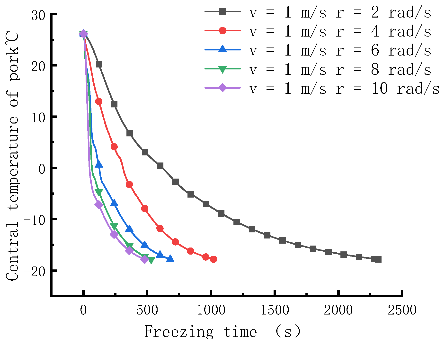
The following information can be obtained from Figure 6. (1) When freezing starts, the central temperature drops rapidly, but at a certain time, there will be an inflection point, and the slope of the curve of the central temperature decline gradually becomes flat. (2) With the increase of refrigerant flow rate, the inflection point will move left along the coordinate axis. This is because when the food is frozen, the free water molecules in the cell will condense into small ice crystals, and the small ice crystals will gather slowly to form ice crystal bands. The freezing time before the inflection point is the time when the largest ice crystal band is formed. The shorter the period, the higher the frozen quality of the food [20]. Deng and Zhu [21] took the change of grass carp in the process of forced convection impregnation and freezing as the research object, and studied the experimental research on the freezing speed and freezing quality of grass carp under the conditions of different flow rates of −20 °C and −30 °C. The experimental results are shown in

Table 6. Flow rate and freezing rate of refrigerant carrier. Reprinted with permission from Ref. [21]. 2012, Deng, M.; Zhu, Z. More details on “Copyright and Licensing” are available via the following link: cnki.net.

Freezing Temperature (−20 °C)		Freezing Temperature (−30 °C)
Current Speed (L/min)	Freezing Rate (cm/h)	Current Speed (L/min)	Freezing Rate (cm/h)
14.9	4.55	12.9	10.57
11.2	3.37	9.9	9.04
8.64	3.06	6.6	8.05
5.88	2.80	4.02	7.24
3.18	2.14	1.02	6.48
0	1.70	0	5.68

. The experimental results are consistent with the numerical simulation results in this paper. With the increase of the flow rate of the refrigerant, the freezing rate increases.

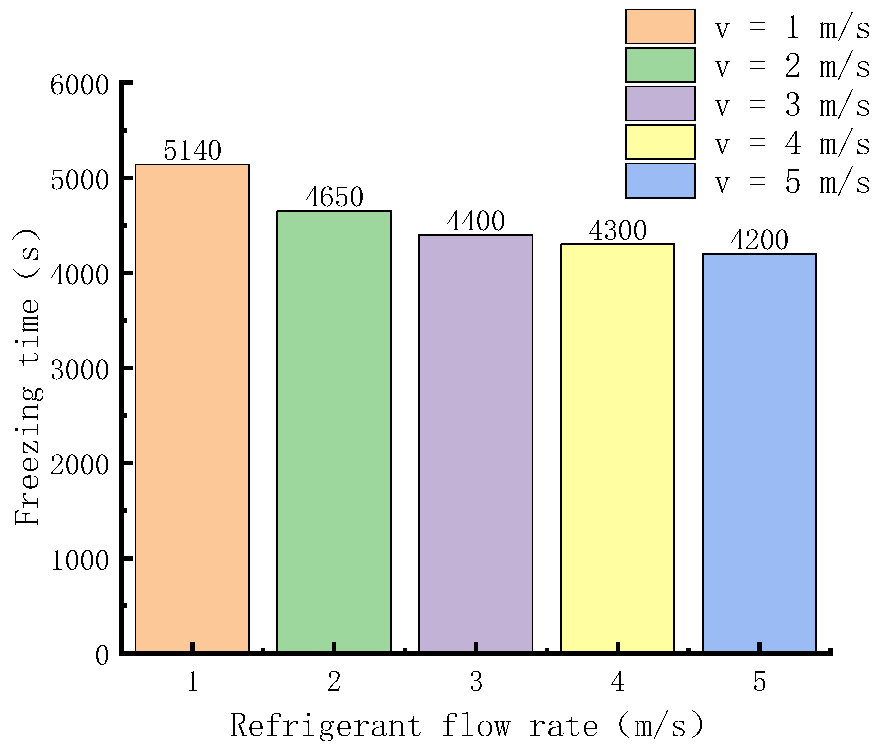
As can be seen from Figure 7, with the increase in the flow rate of the refrigerant carrier, the freezing time gradually decreases. When the flow rate of refrigerant carrier increases from v = 1 m/s to v = 2 m/s, the freezing time decreases from 5140 s to 4650 s (a difference of 490 s), and the freezing efficiency increases by 9.5%. When the flow rate of refrigerant carrier increases from v = 2 m/s to v = 3 m/s, the freezing time decreases from 4650 s to 4400 s (a difference of 250 s), and the freezing efficiency increases by 5.4%. When the flow rate of the refrigerant carrier increases from v = 2 m/s to v = 3 m/s, the freezing time decreases from 4400 s to 4300 s (a reduction of 100 s), and the freezing efficiency increases by 2.3%. When the flow rate of the refrigerant carrier increases from v = 4 m/s to v = 5 m/s, the freezing time decreases from 4300 s to 4200 s (reduced by 100 s), and the freezing efficiency increases by 2.3%. A comparison with existing studies shows that the freezing rate of the immersion frozen samples was higher than that of the air frozen treated samples. Similar results were previously observed in the freezing of strawberries [4]. The freezing process is prone to turbulence phenomena in the liquid medium. This then accelerates the formation of ice nuclei and increases the efficiency of heat transfer. These findings are consistent with the experimental results of Wu on pork [22].

By comparing the temperature program data, it can be seen that increasing the refrigerant flow rate does not affect the freezing effect of pork, that is to say, increasing the flow rate will not change the phenomenon of uneven freezing. From the curve and histogram data, it can be seen that increasing the flow rate of the refrigerant carrier will have an impact on the freezing speed of pork. With the increase of the flow rate of the refrigerant carrier, the freezing time of pork will gradually decrease. However, it can be seen from Figure 8. The improvement of refrigeration efficiency shows a decreasing trend, which means that with the increase of refrigerant flow rate, the improvement of refrigeration efficiency gradually decreases and finally tends to a fixed value.

3.2. Effect of Hopper Rotation Speed on Freezing Time and Freezing Effect of Pork

To further improve the freezing effect, rotation is used to promote a homogeneous freezing process. This aspect is less covered and few studies can be referred to to explain the results.

With the flow rate of the carrier refrigerant constant (v = 1, m/s), five rotational speeds (r = 2, 4, 6, 8, 10) are set to compare the influence of the rotational speed of the rotating hopper on the freezing effect and freezing time of pork. The temperature program in the freezer and the x-y plane temperature program of the different rotational speeds are shown in Figure 9.

Figure 9 shows the temperature distribution in the freezing hopper when the flow rate of the refrigerant is constant and the rotating speed is increasing. Observing the temperature program reveals that the temperature of the refrigerant carrier is kept at the pre-cooling temperature of −20 °C. The temperature of pork gradually increases from the outside to the inside, and the maximum temperature in the center reaches −18 °C. Observing the temperature program of x-y section shows that the temperature gradient of pork is divided into four layers. From outside to inside, the temperature gradually increases. The overall area freezing effect is approximately circular, and the temperature gradient is small. Observing the temperature program and x-y cross-section program at five different rotational speeds, indicates that the program at different rotational speeds is approximately the same. However, compared with Figure 5, it can be clearly seen that when the rotating hopper rotates, the freezing effect of pork is significantly more uniform.

According to Figure 10 and Figure 11 , when the refrigerant flow rate is fixed and the rotating speed is increased from r = 2 rad/s to r = 4 rad/s, the freezing time is reduced by 1290 s from 2310 s to 1020 s, and the freezing efficiency is increased by nearly 55.8%. When the rotating speed is increased from r = 4 rad/s to r = 6 rad/s, the freezing time is reduced from 1020 s to 680 s, which is a change of 340 s, and the freezing efficiency is increased by nearly 33.3%. When the rotating speed is increased from r = 6 rad/s to r = 8 rad/s, the freezing time is reduced from 680 s to 530 s, and the freezing efficiency is increased by nearly 22%. When the rotating speed is increased from r = 8 rad/s to r = 10 rad/s, the freezing time is reduced from 530 s to 480 s, and the freezing efficiency is increased by nearly 9.4%.

Comparing the temperature programs in Figure 5 and Figure 9, it can be seen that when the rotating hopper is rotating, the temperature distribution of frozen pork is significantly higher than that when the rotating hopper is stationary. However, looking at Figure 9, it can be found that the freezing effect of pork does not change significantly with the gradual acceleration of rotating speed. That is to say, the rotation of the rotating hopper can improve the freezing effect of pork, but the rotation speed does not affect the freezing effect of pork.

With the increase of the rotating speed of the loading basket, the time for pork freezing will gradually decrease. It can be seen from Figure 12 that the improvement of refrigeration efficiency will also gradually decrease with the increase of basket speed. This means that it is impossible to shorten the freezing time by continuously increasing the rotating speed. At the same time, the time of the maximum ice crystal band will gradually decrease, and the frozen quality of pork will be improved to a certain extent.

3.3. Effects of Refrigerant Flow Rate and Hopper Rotation Speed on Freezing Time and Freezing Effect of Pork

The same analysis method was used to analyze the effects of refrigerant flow rate and hopper speed on freezing speed and freezing effect. Five groups of simulations were selected: v = 1 m/s, r = 2 rad/s, v = 2 m/s, r = 4 rad/s, v = 3 m/s, r = 6 rad/s, v = 4 m/s, r = 8 rad/s, v = 5 m/s, r = 10 rad/s. The simulation results are shown in Figure 13.

From the above comparative analysis, it can be seen that when the rotating hopper changes from static to rotating, not only is the freezing time reduced, but also the freezing effect is improved and the freezing condition of the product becomes more uniform. However, a single increase in the flow rate of the refrigerant carrier or the rotation speed of the rotating hopper will only reduce the freezing time and will not improve the freezing effect, and the efficiency of the freezing time will gradually decrease with the increase of the flow rate or rotation speed. To sum up, this paper proposes to change the two influencing factors at the same time to observe the freezing time and freezing effect of pork.

It can be seen from Figure 13a that when the flow rate of refrigerant is v = 1 m/s and the speed of the hopper is r = 2 rad/s, the frozen distribution of pork in the center of the x-y cloud is approximately circular. With the gradual increase of the flow rate and rotation speed, the temperature distribution in the center of pork is more and more circular, as shown by Figure 13b–e where it is already a standard circle, and the distribution of freezing conditions is very uniform. This shows that with the constant increase of the refrigerant flow rate and the rotational speed of the hopper, the freezing effect will also gradually improve, and finally achieve the effect of uniform freezing.

According to Figure 14 and Figure 15, when the refrigerant flow rate v = 1 m/s and the hopper speed r = 2 rad/s, the freezing time is 2310 s, and when the refrigerant flow rate v = 2 m/s and the hopper speed r = 4 rad/s, the freezing time is 700 s; the freezing time is reduced by 1610 s, and the freezing efficiency is increased by 69.6%. When the flow rate of refrigerant carrier v = 3 m/s and the speed of hopper r = 6 rad/s, the freezing time is 445 s; the freezing time is reduced by another 255 s, and the freezing efficiency is increased by 36.4%. When the flow rate of the refrigerant carrier v = 4 m/s and the rotating speed of the hopper r = 8 rad/s, the freezing time is 300 s, the freezing time is reduced by 145 s, and the freezing efficiency is increased by 32.5%. When the flow rate of the refrigerant carrier v = 5 m/s and the rotating speed of the hopper r = 10 rad/s, the freezing time is 230 s, the freezing time is reduced by 70 s, and the freezing efficiency is increased by 23.3%.

From the above five sets of simulations, it can be concluded that when the flow rate of the refrigerant and the speed of the hopper are increased at the same time, the time spent on freezing pork can be reduced. At the same time, with the increase of the flow rate of the refrigerant and the speed of the hopper, the freezing effect will become more uniform. However, the improvement of refrigeration efficiency can be seen from Figure 16. With the continuous improvement of the flow rate of refrigerant and the speed of the rotating hopper, the increasing trend of refrigeration efficiency gradually decreases.

Table 7. Record of time taken for the center of the pork to reach −18 °C with changing flow rate and rotational speed.

	Flow Rate (m/s)	1	2	3	4	5
Rotation Speed (rad/s)
0		5140	4650	4400	4300	4200
2		2310	1570	1350	1180	710
4		1020	700	580	505	465
6		680	550	445	340	300
8		530	445	365	300	250
10		480	360	315	280	230

shows the time taken (s) for the center of the pork to reach –18 °C at different combinations of refrigerant flow rate and rotational speed. Figure 17 shows the three-dimensional curved surface of the two variables of freezing speed, flow rate and rotational speed The following conclusions can be drawn from the comparative study presented above when combined with the information in Table 7 and Figure 17: (1) increasing the refrigerant carrier’s flow rate can reduce the freezing time, but the efficiency improvement is minimal, and the effect of the freezing is clearly uneven; (2) Adding a rotating device can significantly reduce the freezing time, increase the freezing efficiency, and significantly increasing the freezing uniformity.

In hydrodynamics, a Reynolds number (Re) < 2300 represents laminar flow, and Re > 2300 shows turbulent flow. Figure 18 and Figure 19 show the velocity nephogram of the flow field when the refrigerant is flowing and the rotating hopper is still. Observing the x-y plane vector diagram shows that the flow field is relatively regular. Obviously, the flow field is in a laminar state at this time. Compared with Figure 20 and Figure 21, when the load hopper is rotating, a turbulent flow field can be seen, indicative of a vortex created in the refrigerant.

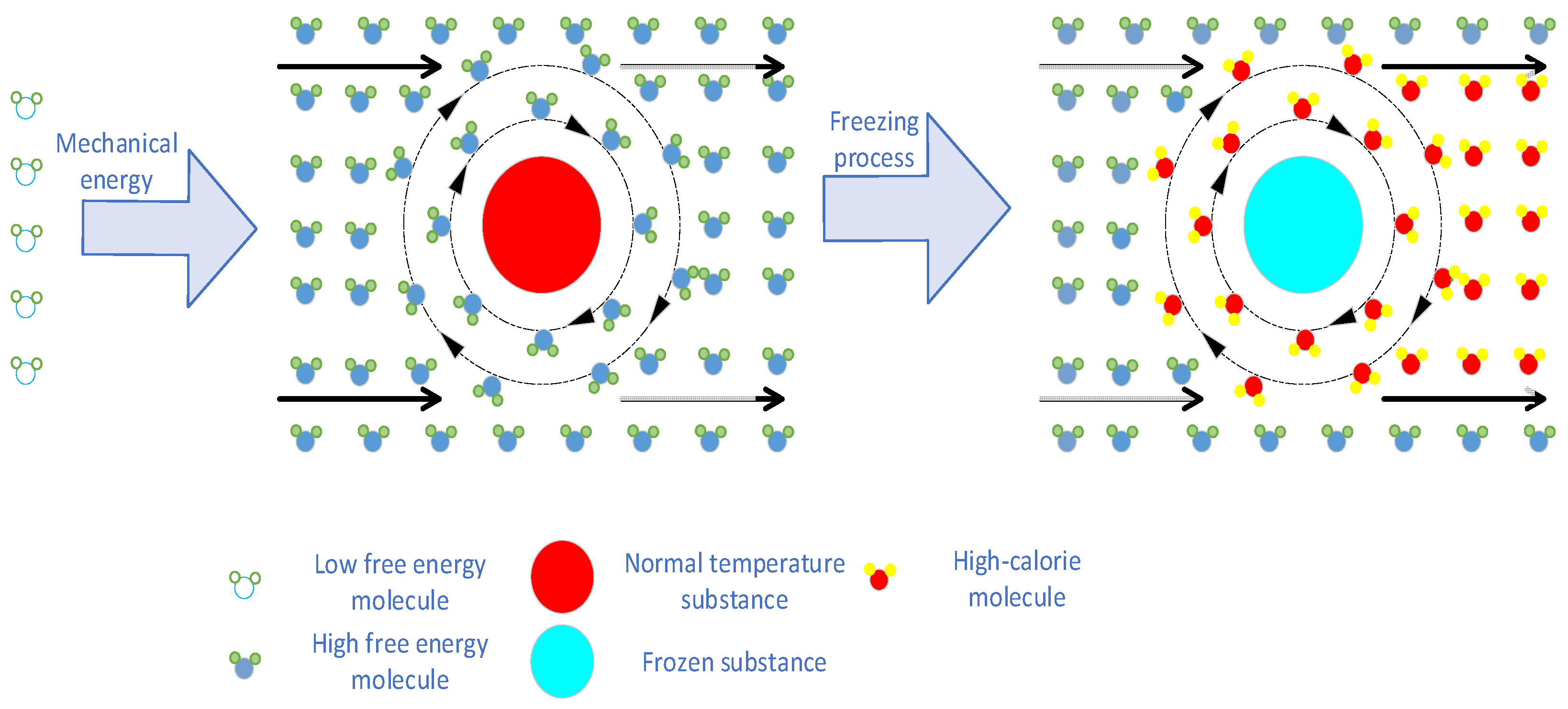
According to the theory of heat transfer, when a fluid flows through a solid surface with a different temperature, the process of heat transfer between the fluid and the solid is called convective heat transfer. When convective heat transfer occurs, the higher the Reynolds coefficient in the flow field, the higher the turbulence intensity, and the more turbulent the flow field. Under the turbulent flow field, the fluid molecules have high molecular free energy. When the solid is in a flow field with high molecular free energy, it is conducive to heat exchange between the solid and the fluid, which in the case of our study is pork and refrigerant fluid, respectively. When increasing the flow rate of the refrigerant carrier and the rotating speed of the rotating hopper, the mechanical energy is converted into the molecular free energy of the fluid via the mechanical equipment, and the flow field becomes more disordered, thus accelerating the energy exchange between the refrigerant and the pork. The schematic diagram is shown in Figure 22.

4. Conclusions

In this work, the idea of including a rotating device is offered to the development of the existing immersion freezing equipment. The new freezing method was computationally simulated using computational fluid dynamics methodology and software, based on the development of a mathematical model.

The enhanced freezing technique and numerical simulation presented in this research offer some theoretical recommendations for the design of immersion freezing machinery. In addition, with reference to Wang’s [23] experiments on different freezing methods of bamboo pod fish, it is shown that brine immersion freezing takes the shortest time and the freezing quality is not high after freezing. The water retention, electrical conductivity, texture, protein and fat quality, and water migration of the helically frozen bamboo pod fish are the closest to those of fresh fish, and the muscle fiber gap is small.

To sum up, the new freezing method proposed in this paper can not only greatly reduce the freezing time, but also improve the non-uniformity of the existing refrigeration equipment. If this technology is applied to the industrial process of freezing food, it can improve the industrial production efficiency, increase the quality of industrial production, and provide strong quality assurance for the subsequent cold chain transportation. In addition, the improved freezing method and numerical simulation in this paper provide some theoretical guidance for the development and research of immersion refrigeration equipment.