Article

Use of Land Gravity Data in Small Areas to Support Structural Geology, a Case Study in Eskişehir Basin, Turkey

Institute of Earth and Space Sciences, Eskişehir Technical University, Eskişehir 26555, Turkey
*
Author to whom correspondence should be addressed.
Appl. Sci. 2023, 13(4), 2286; https://doi.org/10.3390/app13042286
Submission received: 20 December 2022 / Revised: 3 February 2023 / Accepted: 4 February 2023 / Published: 10 February 2023
(This article belongs to the Special Issue Recent Advances in Geospatial Big Data Mining)

Abstract

:
Various researchers have contributed to the literature on the locations and lengths of existing faults in the Eskişehir Basin, Turkey. However, the majority of the literature on the subject bases its results on fault indications observed on the surface, for example, surface ruptures. In addition, studies using geophysical methods in order to reveal buried faults have also fallen short regarding depth compared to gravity. In order to have a better understanding, the gravity method was applied with a total of 448 gravity measurements on five parallel lines in the north–south direction of the study area, which also includes the urban area of the Eskişehir Basin. Considering the neotectonics of the Eskişehir basin, the measurement lines were chosen to perpendicularly cut the east–west extending faults of the Eskişehir fault zone. For the first time in the literature, a detailed Bouguer gravity anomaly map has been obtained for the Eskişehir Basin using land gravity measurements. The edge detection Horizontal Gradient Magnitude (HGM) and Euler Deconvolution (ED) methods were applied to obtained Bouguer anomaly data. Both of these use spatial analysis of Bouguer gravity anomalies. An HGM map shows the presence of maximum amplitude areas in the south and north of the study, and these areas were found to be compatible with the known faults in the literature. ED solutions also support HGM maximums. The relationship between the lineaments obtained from the edge detections and the seismicity of the region were examined. It can be seen that the results obtained from both the HGM and ED edge detection methods are highly compatible with each other, and highly related to the structural geology of the region. Although great agreement with the faults in the literature was determined by both methods, only the ED method showed a number of newly found faults in the area. In addition, the locations of the known faults in the region were supported by the geo-physical gravity method for the first time.

1. Introduction

The Eskişehir Basin is a disaster-prone area due to the earthquake hazard, non-earthquake-resistant buildings, and local ground conditions [1]. Seismic hazard analyses have been investigated in previous studies, and seismic hazard maps have been produced using the locations of earthquake that occurred between 1900 and 2019. The lengths of active faults in the region were then determined, along with the earthquake magnitudes that could be generated by those faults in order to assess the earthquake hazard in the study area [2].
The Eskişehir Fault Zone (EFZ) in the study area is one of the internal fault zones of the Anatolian Plate [3,4,5,6]. It is closely related to the Eskişehir Basin [7,8,9]. The locations of active segments in the EFZ, and the source of the Ms 6.4 magnitude earthquake that occurred on 20 February 1956 (one of the main seismic events in the region), have been discussed in detail in the literature [4,8,10,11,12]. Seyitoğlu, Ecevitoğlu, Kaypak, Güney, Tün, Esat and Uyar Aldaş [11], in one of the most recent studies conducted in the region, found that the Çukurhisar-Sultandere fault segment passes to the south of Eskişehir city center and is considered to be one of the important earthquake sources in the region. Liquefaction and soil amplification are the leading earthquake-related risks that are features of the region. To further support the structural geology and reveal seismic risks in Eskisehir, Graben gravity measurement points of five lines, each starting with a southernmost station, have been planned (Figure 1a). Eskişehir city center is rated as high to moderate with regard to soil amplification and liquefaction hazards [1] (Figure 1b). The study area mainly consists of old and new alluvium, which is bounded by hard rocks (limestone, conglomerate, ophiolitic mélange, and marble) in the north and south [11,13,14] (Figure 1b).
Determination of active fault locations in the region is extremely important in terms of earthquake hazard assessment. It has been seen in previous studies that gravity measurements produce successful results in determining horizontal discontinuities [15,16,17,18,19,20,21]. Bouguer gravity anomaly maps also reveal information regarding plunging or vertical lateral boundaries between rock units. Detected boundaries are generally interpreted as horizontal discontinuities of features, such as geologic contacts, faults, or horsts/grabens. The most important purpose of the edge detection analysis of this study is to detect such discontinuities, which are usually masked in Bouguer maps. The fault locations, which can be revealed by two-dimensional edge detection, provide significant additions for later seismic reflection and paleoseismology studies. In addition, the Bouguer gravity anomaly map obtained in the study area, a region rich in geothermal resources, will contribute to preliminary evaluations to be made within the scope of geothermal exploration [22,23,24,25,26].
The aim of this study is to carry out edge detection of data collected in the field by gravity measurements to reveal the fault structures that form the Eskişehir Graben (Figure 1a). Previous studies in the region have used a variety of methods, such as geological observation, boreholes, seismic reflection and microtremors, to reveal the structural geology of the Eskişehir Basin [4,11,27,28]. However, these methods listed above either rely only on surface observations (for example, surface ruptures and geological discontinuities) or provide shallow results compared to the gravity method. Within the scope of the study, two edge detection methods, namely, horizontal gradient magnitude (HGM) and Euler Deconvolution (ED), were applied to high resolution field gravity data, and the results of the methods were examined against each other and the literature for consistency.

2. Geological Setting of the Study Area

Many studies and compilations have been carried out in the past to determine the geological features of the Eskişehir graben [8,10,14,29,30,31,32,33,34,35]. According to these studies, the existing formations from youngest to oldest within the provincial borders of Eskişehir are Alluvium, Akçay Formation, Ilıca Formation, Porsuk Formation, Mamuca Formation, and Karkın Formation.
In general, Triassic metamorphic schist–marble and ophiolitic mélange constitute the oldest units of the study area. Eocene-aged conglomerate, marl, limestone, claystone, Miocene-aged andesite, conglomerate, clay marl, and limestone, and tuff, Pliocene clay, tuff, and basalt series are found on these oldest units in the region with angular unconformities. At the top are old and new alluvium [32]. In the study area there is Pleisto-cene-aged alluvium containing gravel, sand, silt and clay, Akçay Formation, conglomer-ate-sandstone, limestone, and marl, as well as Pliocene-aged Ilıca Formation containing basalt, tuff, clayey tuff limestone, and conglomerate-sandstone. It can be seen that clayey tuffaceous calcareous levels of Pliocene-aged Ilıca Formation crop out within the Porsuk Formation. Orogenic movements and faulting have been effective in taking the current shape of the graben. As a result of the faulting, the south and north of the Eskişehir region show uplift behavior, while the middle part takes the form of a graben and forms a young series.
It can be said that the Eskişehir Basin is a region with tectonic regime characteristics controlled by graben systems bounded by normal faults in the north and south. It is known that there is Quaternary-aged sediment (alluvium, old alluvium) with a deepest point of 100 m in the Eskişehir Graben. Morphometric studies show that the northern faults of the graben are as active as the southern faults, and that the ongoing strain affects the fluvial features of the region [8].
It is known that the Eskişehir region consists of two main structural units, namely, the northern assemblages and the southern assemblages, which describe the original tectonic environment. Although the base of the basement rock is unknown, it has been interpreted that it continues with recrystallized limestones [28].

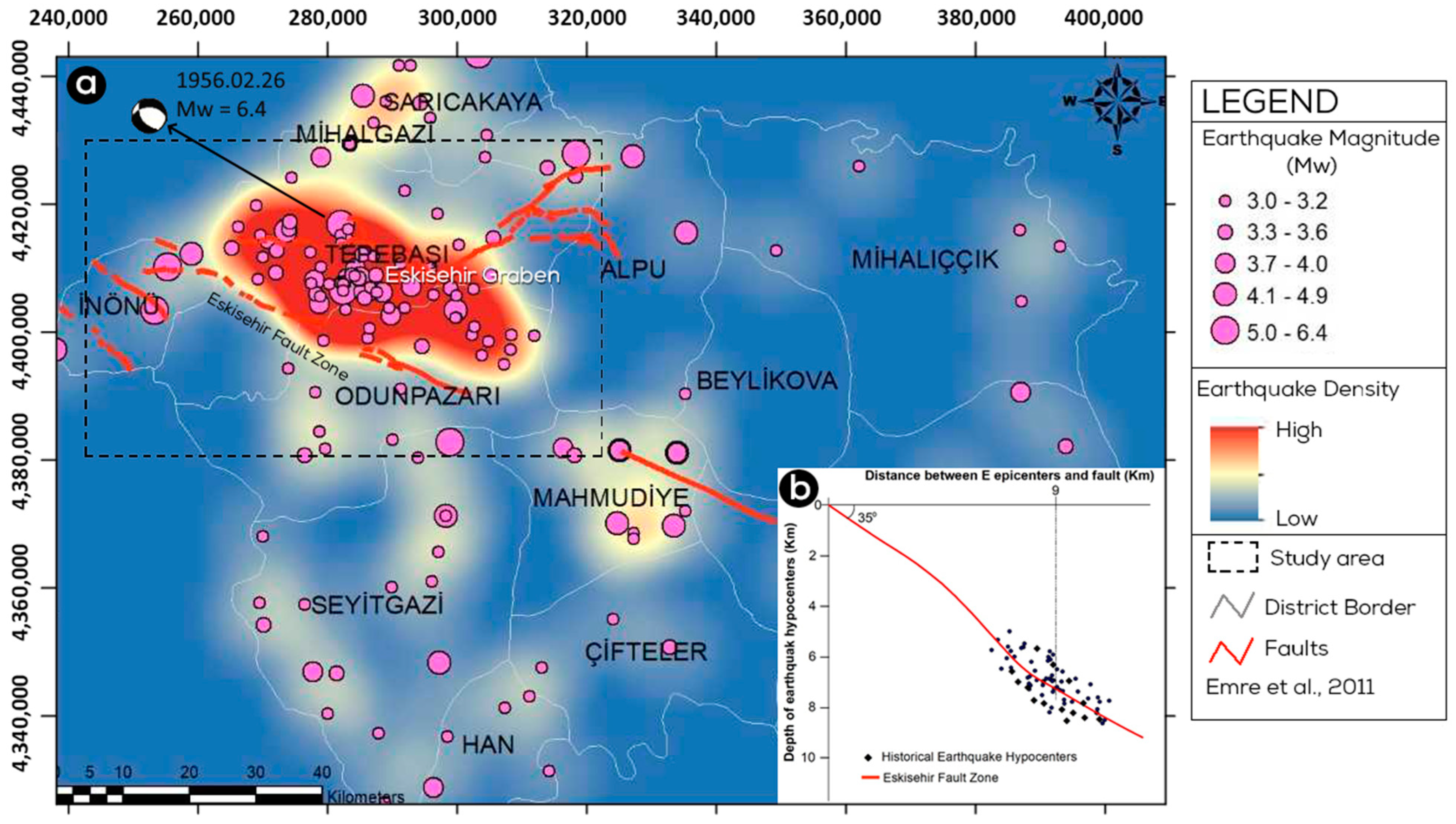
3. Earthquake Distribution in the Study Area

The aim of this section is to review all of the historical and instrumental earthquakes in the Eskisehir region, between 1900 and 2019, to determine the earthquake density within the Eskisehir Province and also to delineate the regions characterized by earthquakes of different depths. A map was generated for that purpose using ArcGIS 10.5; An Earthquake Density Map of Eskisehir (1900–2019) (Figure 2a).
Earthquake data from the years 1900–2019 were downloaded from the KOERI (Kandilli Observatory and Earthquake Research Institute) web portal (url-1: http://www.koeri.boun.edu.tr/sismo/zeqdb/ accessed on 8 March 2022). During the downloading, all of the parameters were selected as accurately as possible with coordinated boundaries to cover the Eskisehir Province for earthquakes with magnitudes greater than 3. There were 161 earthquakes in total with magnitudes of greater than 3 that occurred within the study area within the selected time span.
The result of the analysis shows that most of the earthquakes with magnitudes between 3 and 6.4 occurred in the southern part of the Tepebaşı District and the northern part of the Odunpazarı District. The earthquake occurrence is attributed to faults, because most of the earthquake epicenters are distributed between active faults. Generally, the northwest regions of the Eskisehir Province are characterized by a high density of earthquakes, and the center and southwest regions are accompanied by moderate numbers of earthquakes, while the northeast and east parts are characterized by a low density of earthquakes. This distribution has a high correlation with active faults, as the regions with high earthquake density are also occupied by active faults (Figure 2a).
As shown in Figure 2, the EFZ trends from northwest to southeast, and most of the earthquake epicenters are located within that zone. The faults have parallel distribution to the fault zone orientation. To find the dip of the Eskisehir Fault Zone, the earthquake hypocenters first were located by finding the distance of the earthquake epicenters from the fault zone and their depths below the surface. The average distance between the earthquake points and the zone was calculated and found to be about 9 km. The average depth of earthquakes that have occurred around the fault is between 5 and 10 km. The dip of the EFZ was calculated graphically and is shown in Figure 2b. The result of the calculation shows the EFZ to be dipping about 35° to the northeast.
The seismicity map of the study area and its surroundings and the location of the 20 February 1956 (Ms 6.4) Eskisehir earthquake are presented in Figure 2a. In all, 3499 houses, 10 schools, 15 mosques, and 3 official buildings were demolished, along with 1303 barns and haystacks in that particular earthquake in Eskişehir city center. In the 17 August 1999 Kocaeli (Mw 7.4) earthquake, which was centered approximately 250 km from Eskişehir city center, 86 people lost their lives in the city of Eskişehir, and 95 people were injured. In addition, 70 houses/workplaces suffered severe damage, 1 building collapsed during the earthquake, and 4 buildings collapsed after the earthquake [37].
According to the AFAD (Disaster and Emergency Management Authority) 2018 Earthquake Hazard Map of Turkey, the highest ground acceleration that can be encountered in the study area, with a 10% probability of exceedance within 50 years (return period of 475 years), is determined to be 0.29 G (url-2: https://tdth.afad.gov.tr/ accessed on 8 March 2022). The formation of lacustrine basins that occurred in the early Miocene was probably controlled by dip-slip normal faults striking in an east–west direction as a result of tensile stress in the north–south direction. Later, as a result of the northwest–southeast directional pressure stress affecting the region, strike-slip faulting developed and caused the previous dip-slip fault planes to break [34]. The Eskişehir Fault Zone began to appear in regional maps in various studies in the literature [3,38,39]. Later, the EFZ was investigated and divided into the Dodurga, Kandilli, İnönü, Osmangazi, and Kaymaz segments [40]. Barka, et al. [41] state that the Eskişehir Fault starts near Bursa in the west and extends to the east of Sivrihisar. They state that this fault is of great regional importance in that it is the main geological element that separates Central Anatolia, which is characterized by strike-slip faults, from Western Anatolia and the Aegean Region, wherein expansion is accommodated with normal faulting and affects a much larger area. Altunel and Barka [10] first named this line extending from Bursa to Kaymaz the ‘Eskişehir Fault Zone’ (EFZ).

4. Methodology

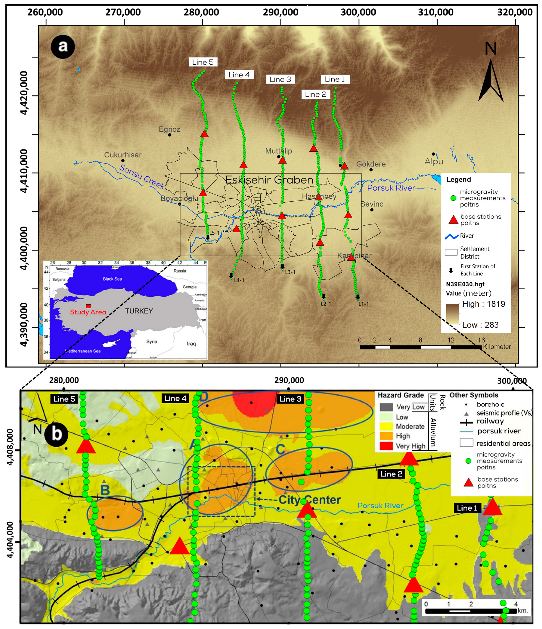
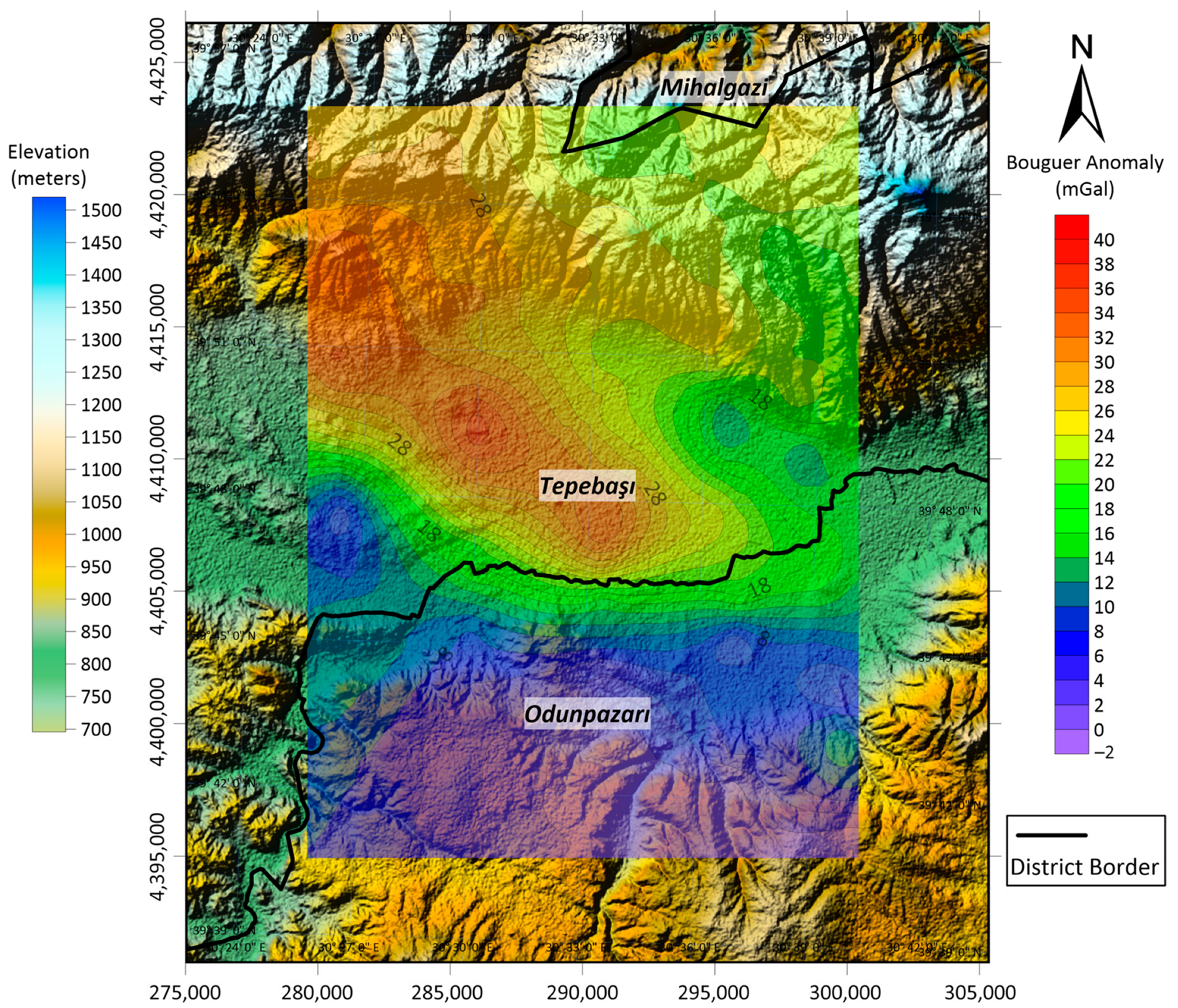
4.1. Gravity Field Survey and Bouguer Gravity Anomaly Data

Through east-to-west-oriented active fault segments in the northern and southern parts of the Eskişehir, Graben played an important role in the formation of the depression area [4,11,14]. Therefore, discussing the fault system controlling this structure with edge detection using microgravity data makes a significant contribution to the geological setting of the region. For this purpose, five lines approximately 4 km apart were chosen along a 30 km long region. The lines are in a north–south direction and perpendicular to the fault systems, and the distance between the gravity measurement points was designed to be 200 m following the Nyquist rule (Figure 1a). The Nyquist rule states that the shortest wavelength that can be measured is twice the distance between the measuring points, which is 0.4 km in our study [42]. Gravity measurements were made at an average of 100 points along each line. Three measurements of sixty seconds were taken at each measurement point, and the measurement with the least noise and standard deviation was used for each point. A CG-5 automatic gravimeter, used to collect gravity data, calculated standard deviation and error values automatically for every sixty seconds long measurement. The reliability and accuracy of each measurement were analyzed by base measurements. If there was a large difference between the two base measurements, it was accepted that there was a problem with the device, and the measurements between the two base measurements were repeated after the device was checked. To correct the drift error, twelve base points were established along the lines within the measurement area (Figure 1a). The first base point was chosen twenty points north of the beginning of the line 1. In addition, high-precision location coordinates were obtained with an RTK (Real Time Kinematics) GPS device. The measurement location code, measurement time, weather conditions, and other environmental conditions were entered into a gravity measurement form at each measurement point. Each working day began with a measurement at the base point, and ended with a base measurement. To minimize the drift error in the measurements, the measurements were taken by returning to the base point every two hours.
Each station’s corrected Bouguer anomaly value was obtained by applying corrections for elevation (free air and Bouguer plate corrections), drift, latitude, tide, and terrain. A Bouguer anomaly map of the study area was obtained by gridding single station data using the Kriging method (Figure 3) (Data S1 [43]). In order to apply Bouguer plate correction and terrain correction, the average density of the study area was chosen to be 2.67 gr/cm3 considering major surface geological units, which is also the average density of the upper crust. The physical and mathematical foundations of the gravity corrections have been discussed extensively by numerous authors, so just brief information is given about the corrections [44,45].
An RTK GPS device connected to an active CORS (Continuously Operating Reference Stations) network was used at each measurement point in order to make the most accurate elevation corrections. The sensitivity of the device is about ten centimeters horizontally and about thirty centimeters vertically. The precise elevation reading of each measuring point is used for elevation corrections. After each measurement, the height of the device was also measured by a laser meter. Therefore, the exact height of the sensor inside the device was calculated. By the elevation data, the correction values were applied in the most accurate way according to the conditions at hand.
The United States’ Geological Survey’s (USGS) Earthexplorer SRTM DEM data were used for terrain corrections and calculated for each measurement point using the Geosoft OASIS Montaj program (url-3: https://earthexplorer.usgs.gov/ accessed on 17 May 2018). In order to apply the best corrections, SRTM 1-Arc Second Global was used as topography reference. The cell size of the raster data is 1-arc second, which is approximately thirty meters inside the study area. The Oasis Montaj program uses the vertical prism method for terrain correction [46]. In order to apply terrain correction with the vertical prism method, two nested areas were determined to facilitate the calculations. The topography height data of more frequently sampled inner area and less frequently sampled outer area were prepared. The reason behind this process is that the effect of the inner area on the measured gravity value is much greater, and the topographic changes in the outer area are relatively ineffective [46]. In this study, the center of the study area was accepted as being the center of the inner and outer circle; the radius of the inner circle was chosen to be fifty kilometers and the radius of the outer circle was chosen to be one hundred and fifty kilometers. The Bouguer anomaly map does not reflect the features of surface geology, but it is related to lateral changes in density, depending on the depth. Therefore, Bouguer anomalies are expected to reflect all heterogeneities of subsurface geological structure and density. The Bouguer anomaly map shows northwest–southeast trending gravity contours. The trend from the northwest to the center of the study area is characterized by high gravity values.

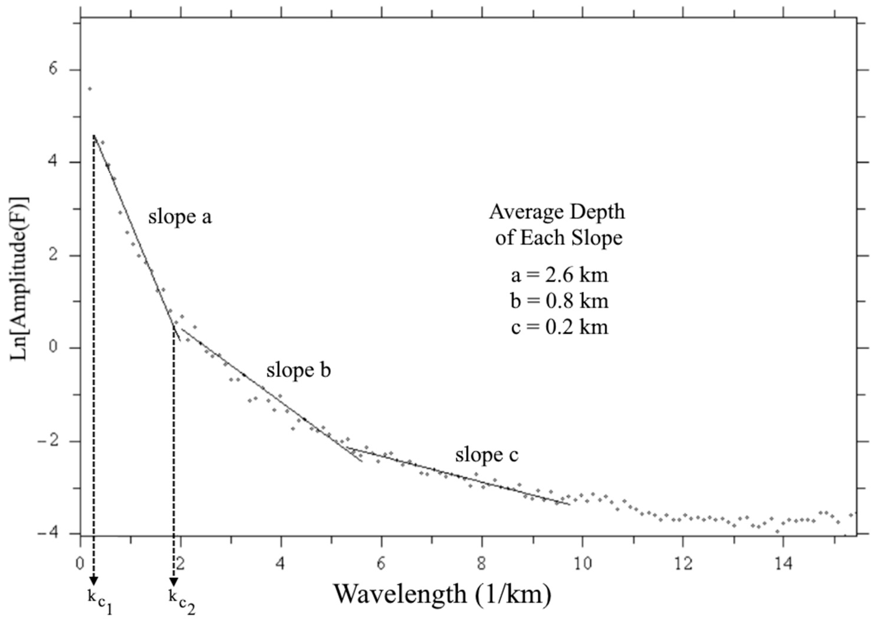
4.2. Spectral Analysis
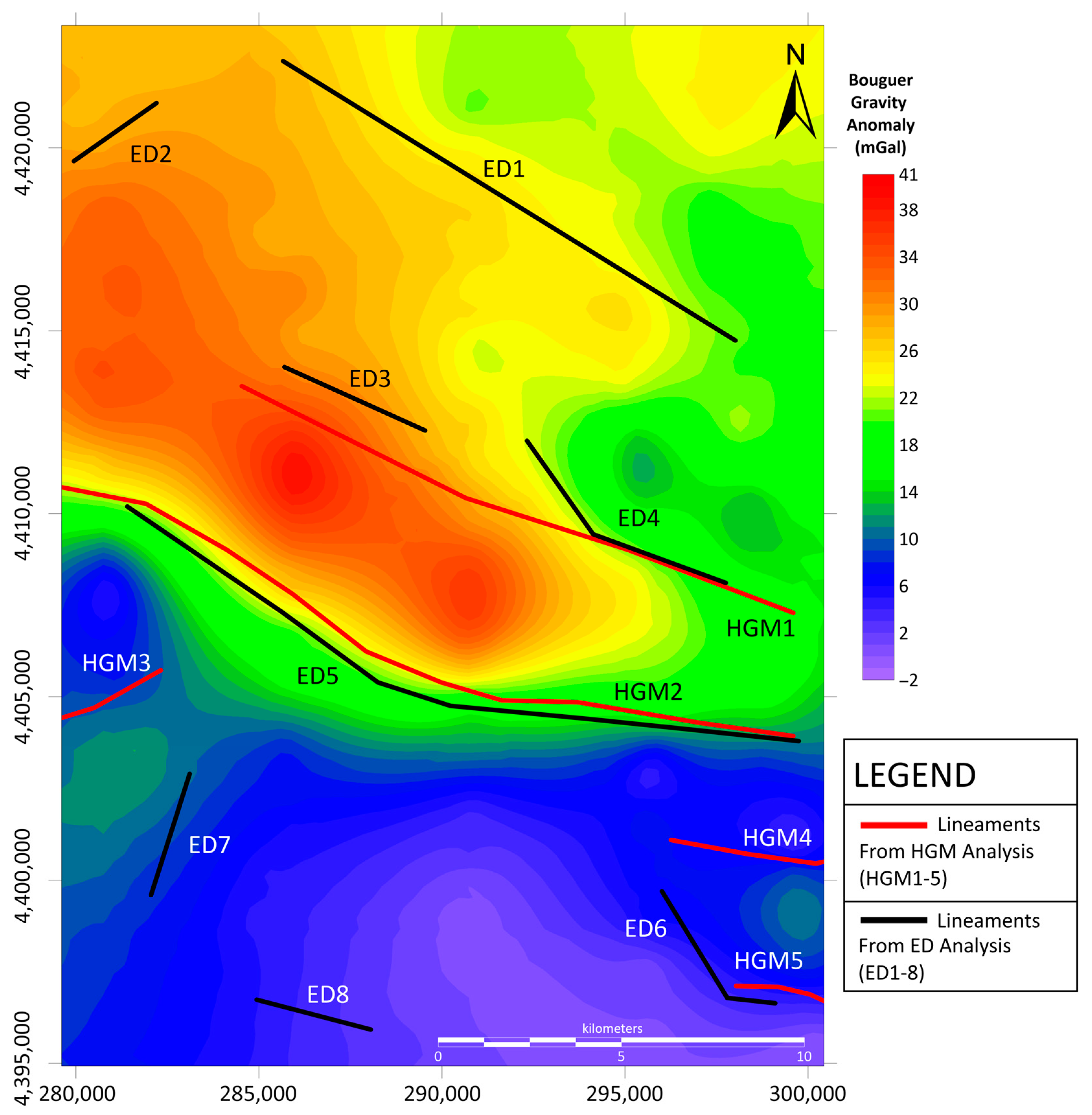
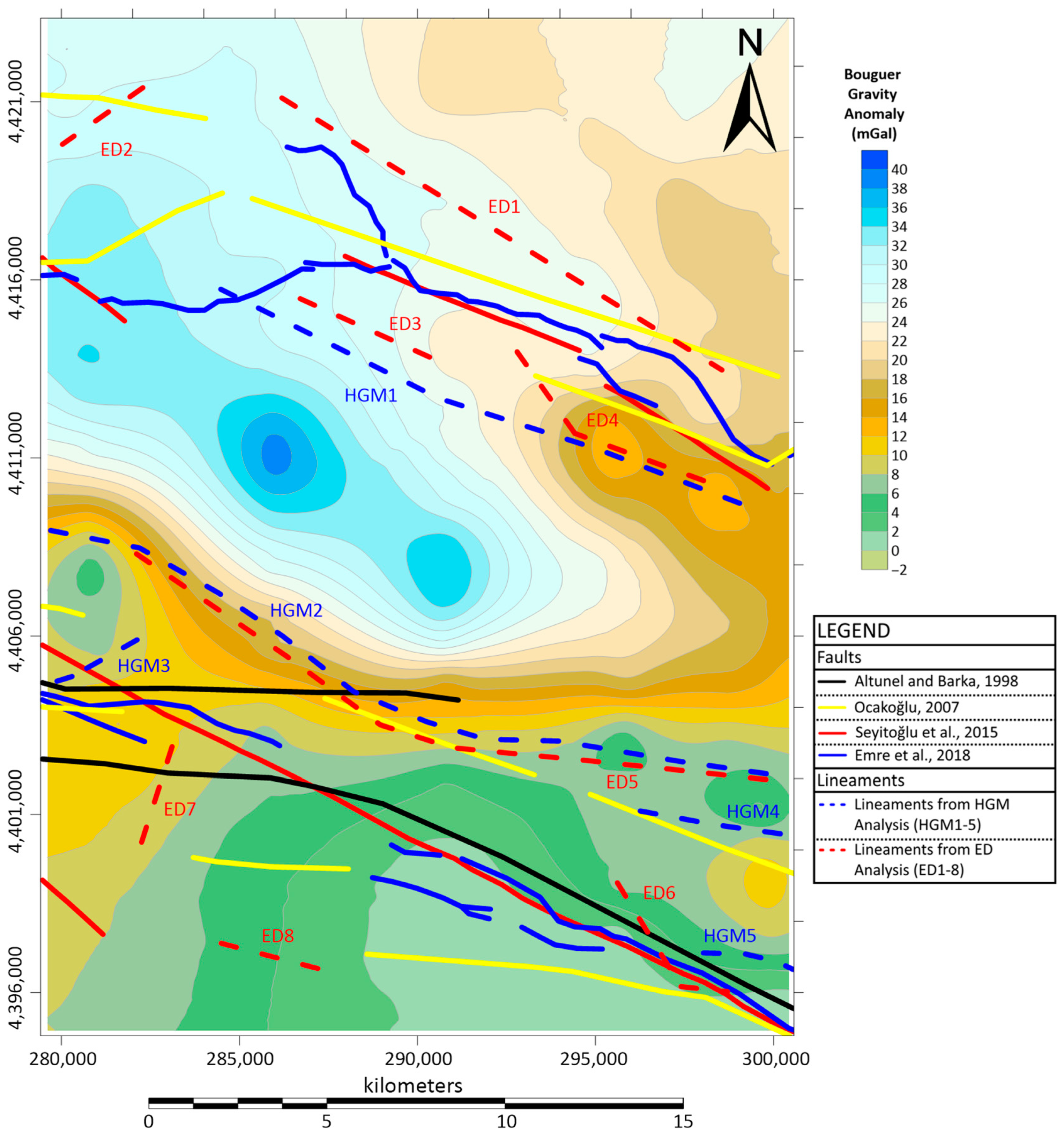
With the help of spectral analysis of the gravity data, average depths of underground layers can be calculated without requiring any geological or density information about the region.
The radial amplitude value (Equation (1)) is obtained by calculating the amplitude spectrum obtained as a result of the two-dimensional Fourier transform around a circle with the center point of ( k x = k y = 0 ) and radius of k r (Equation (2)).
A = F = Re ( F ) 2 + Im ( F ) 2
k r = k x 2 + k y 2
The amplitude spectrum is generally used to calculate the depths of the upper boundaries of potential field sources [47]. Therefore, the natural logarithm of the radial amplitude spectrum was taken and plotted on a graph against the wave numbers. Lines were drawn manually on the decreasing-amplitude curve, and the slopes of these lines gave the average depth of the layers (Figure 4). Fourpot 1.3b application was used for the analysis [48].
On the basis of the critical wave numbers obtained as a result of spectral analysis, the average lower and upper boundary wavelengths of the layer of interest for the study area were calculated to be 3.22 km and 18.5 km (Equations (3) and (4)).
k c 1 = 0.34   rad / km λ c 1 = 2 π k c 1 = 2 π 0.34 = 18.5   km
k c 2 = 1.95   rad / km λ c 2 = 2 π k c 2 = 2 π 1.95 = 3.22   km

4.3. Edge Detection

In gravity and magnetic methods, geological discontinuities are generally defined as potential field linearities. Linear structures in gravity anomaly maps are mainly characterized as sudden changes occurring along a single line or as broken lines defined as gradient regions. In this study, the horizontal gradient magnitude (HGM) and Euler Deconvolution (ED) methods were used to reveal the positions of the above-mentioned gradient regions. The sudden gravity changes detected in the HGM and ED methods correspond to structures, such as geological contacts or faults.

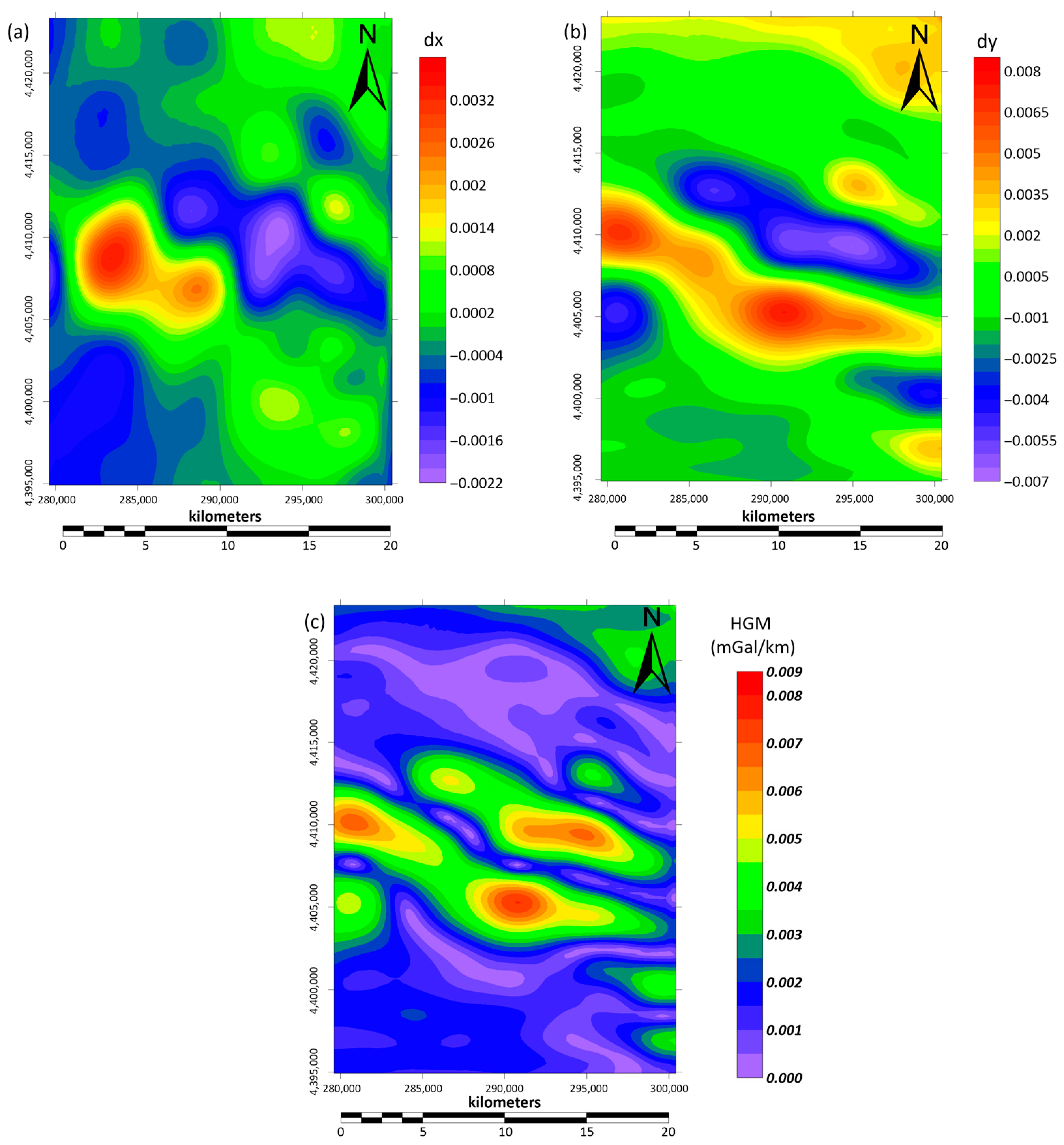
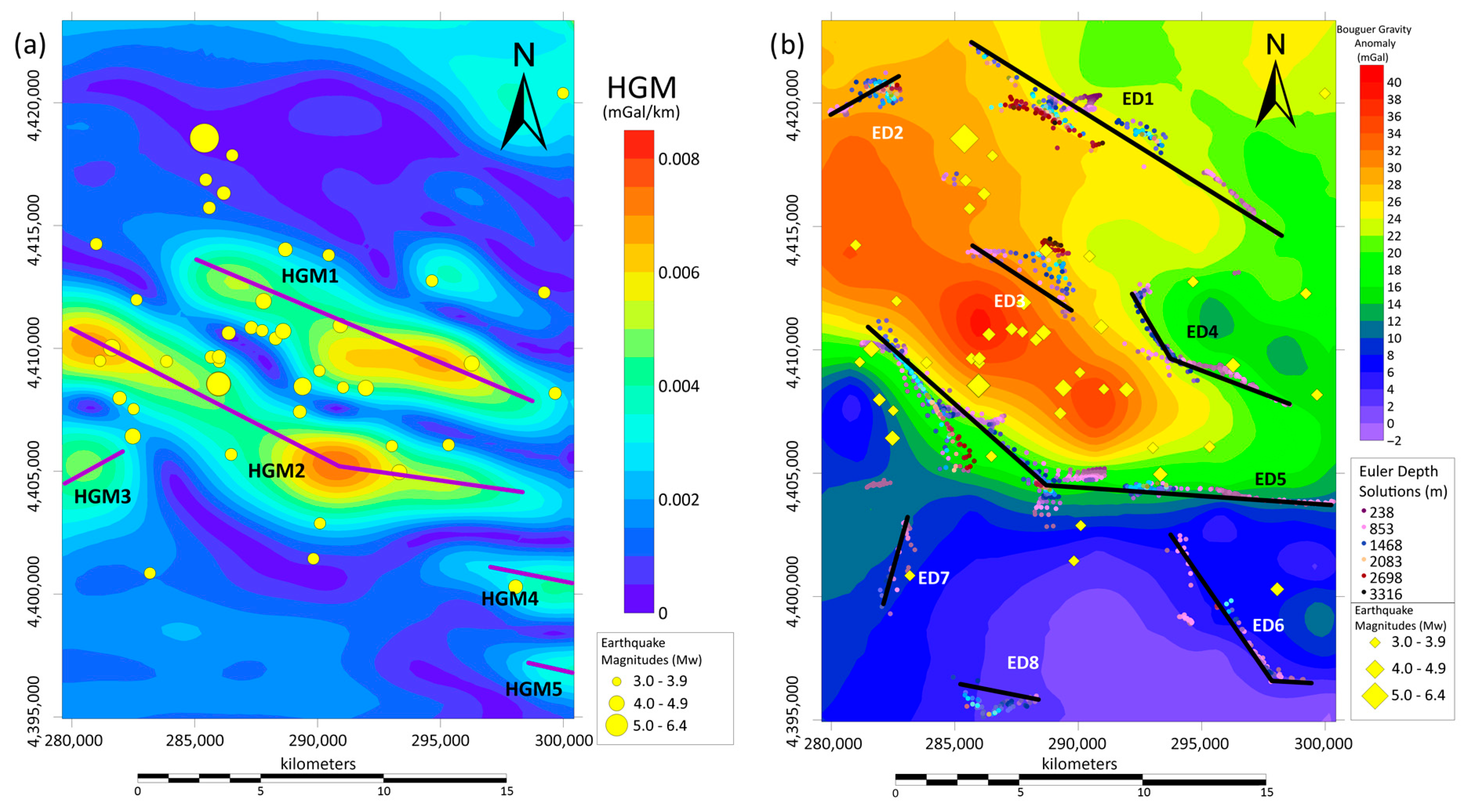
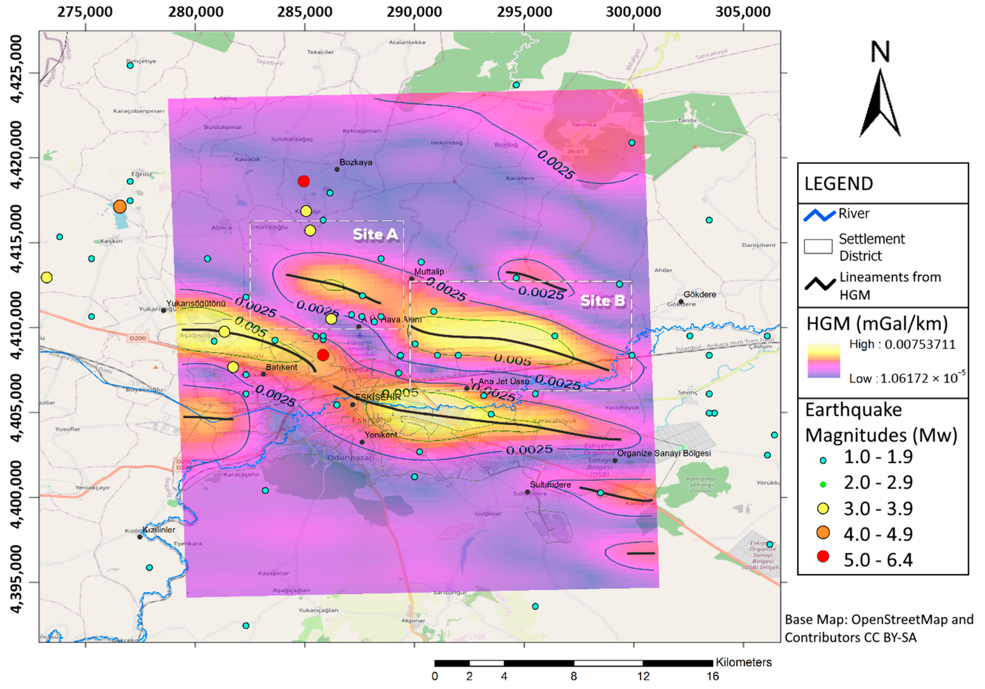
4.3.1. Horizontal Gradient Magnitude (HGM)

The method based on the magnitude of horizontal derivatives of gravity anomalies (HGM) was first proposed by Cordell [49]. The principal advantages of the method are that it does not require vertical derivatives, and that the horizontal derivatives can be easily calculated in the spatial domain. HGM data are shown as the square root of the sum of the squares of the first horizontal derivatives in the x and y directions of gravity anomaly maps (Equation (5)):
H G M ( x , y ) = g ( x , y ) x 2 + g ( x , y ) y 2
The method is based on determining only the regions in which the HGM is maximum along the grid data of the gravity anomaly map. The maxima of the HGM are particularly effective in determining vertical or approximately vertical density boundaries, faults, and geological contacts. Another advantage of the method is that the HGM maxima can be calculated with better sensitivity to noise effects. The HGM method has been discussed and used in various ways by numerous researchers [15,49,50,51]. Solutions can be produced for both shallow and deep boundaries using the HGM method. The disadvantage of the method is that if the borders diverge from the vertical and are very close to each other, the HGM maxima do not occur on those limits.
First, the Bouguer gravity data had to be filtered, and then, the first, second, and third-order trend data were removed, respectively. The focal depths of the earthquakes caused by the earthquake-forming faults in the study area vary between five and ten km when earthquake distribution is considered. To eliminate the effect of deep structures and to reveal the effects of shallow structures with possible lineaments, a low-pass filter was first applied to the Bouguer anomaly data. The HGM method applied to each trend removed items of data one by one. On the basis of the observations made, it was decided that the third-order trend-removed solution was the preferred result to continue interpretation. The HGM map was prepared by taking the square root of the sum of squares of the x-directional first derivative (Figure 5a) and the y-directional first derivative (Figure 5b) of the filtered gravity anomaly. The HGM results show shallow structures in the study area that display linearity. The maximums of the HGM indicate possible lineaments. Fault-type structures and mass boundaries presenting density differences in certain parts of the study area can also be seen on the HGM maps. Upon examining the HGM map, it can be seen that there are maximum amplitude areas in the southern and northern regions of the study area (Figure 5c).
The maximum amplitude values of the HGM were determined to be compatible with the characteristics of the tectonic discontinuities of the Eskişehir Fault Zone in the north and northwest regions, and with the form of short, far from systematic, scattered maxima in the north (Figure 5c).

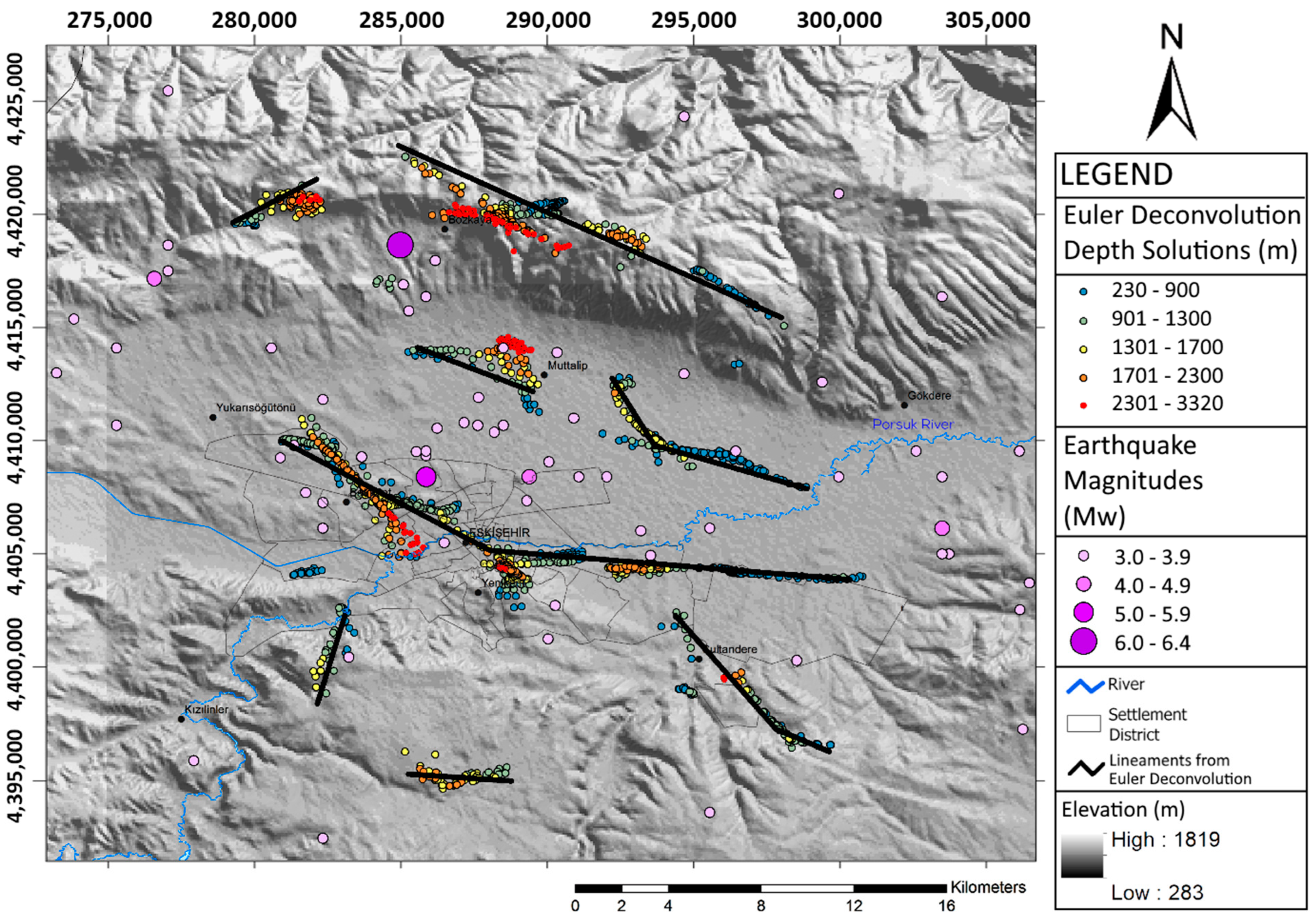
4.3.2. Euler Deconvolution (ED)

The standard Euler method is based on Euler’s homogeneity formula. The formula relates the (gravity) potential field and gradient elements to the location of the source, according to a certain degree of homogeneity (N), which is called the structural index [52]. This system produces results by solving the Euler equation for sub-grids (windows) within a grid using the least squares method. The most important step of the method is the choice of the correct structural index value. When choosing the window size, it is appropriate to choose a window size that includes a certain anomaly, but one that does not include other anomalies in the calculation. Thompson [52] provided a short explanation to describe Euler’s equation. A homogeneous three-dimensional equation of degree t (as any real number) fits the following equation (Equation (6)):
f ( t x , t y , t z ) = t n f ( x , y , z )
Thompson [52] showed that another equation of Euler is also applicable here (Equation (7)):
x g x + y g y + z g z = n f
Considering the potential field data, the final Euler homogeneity relationship is shown as (Equation (8)):
( x x 0 ) g x + ( y y 0 ) g y + ( z z 0 ) g z = N ( B T )
In this formula, x 0 , y 0 , and z 0 are the gravity source coordinates; g is the measured potential field density in the x, y, and z coordinates; N is the structural index describing the geometry of the structure; and T is the total area determined in the x, y, and z coordinates, that is, the regional area B is the sum of the Δ T changes created by the source. T is also expressed as in Equation (9):
T = Δ T + B
Thompson [52] and Reid, et al. [53] state that the choice of structural index is extremely important. Both studies defined the structural index as the rate of change of an area based on distance. They also defined the structural index according to certain structures. It has been seen that the structural index for gravity, N, takes values between 0 and 1. As a result of the calculations, it was determined that N = 0 and N = 1 are suitable for fault structures and that N = 2 is suitable for global anomaly sources (Table 1).
Euler’s Deconvolution method has been shown to be a suitable and interesting method for the purpose of this study. It offers a more advanced and wider solution than other methods because the method offers the opportunity to reveal the structural geology within any zone. The success of the application of the method used in this study was thoroughly examined [54,55,56,57,58].
The various window widths and tolerance percentages were tested in the process of Euler deconvolution. Because the main purpose of the study is to reveal buried faults (step structure) in the Eskişehir Basin and we used Bouguer gravity anomaly as input data, N = 0 was chosen as the structural index (Table 1). Since the aim of the study was to explore buried lineaments, the window size selected was 1 km, and the tolerance percentage was selected as T%, was 15%. Window sizes larger than 1 km caused clustering and scattering of ED solutions. After the parameters had been selected, the Bouguer anomaly map was processed with the help of the Oasis Montaj application, and Euler Deconvolution solutions were obtained and mapped (Figure 6).

5. Results and Discussion

Although microtremor [59] and seismic reflection [11] studies were carried out in previous studies, the first field gravity measurements of the region were made and a detailed Bouguer gravity anomaly map of the region was obtained. As mentioned in the introduction, the obtained map is detailed enough to be used in many studies, such as geothermal studies. Furthermore, previous studies were shallow compared to the data that has been obtained in our study. Tün, Pekkan, Özel and Güney [59] provided a research depth of approximately 800 m using microtremors and seismic reflection. Since the main source of the gravity method is the Earth’s gravitational body forces, we managed to gather data from as deep as 3.22–18.5 km, and this is explained in the ‘Spectral Analysis’ section. As shown in Figure 2b, the average depth of earthquakes occurring in the basin is around 8–10 km, which falls inside our data limits.
Although gravity measurements were performed on hard rock units in the north and south of the site, contrary to expectations, it presents relatively positive anomalies in the north, but negative anomalies in the south (Figure 1b). The source of these anomalies may be a much deeper tectonic structure. Further geophysical and geological studies could be conducted to reveal the nature of these anomalies.
The lineaments obtained from the HGM method of the study area and the lineaments obtained from the ED method were evaluated comparatively, and the consistency of those lineaments with the seismic activity in the region was examined. Linearities obtained by the results of the analysis were compared with the current earthquake locations that have been documented in the Eskişehir Basin. Earthquakes occurring between 1900 and 2019 were used for the study (Figure 2). In order to prevent the map from becoming overcrowded and unreadable, earthquakes with a magnitude of Mw 3.0 and above were compiled. At the same time, earthquakes with a magnitude of Mw 3.0 and above provide more consistent depth and location solutions for the study area. In total, forty-nine earthquakes were mapped within the framework of the mentioned criteria.
There is a remarkably compatible relationship between the results of the edge detection analyses obtained from both the HGM and ED methods and the locations of the earthquakes in the region (Figure 7). However, if the determined lineaments represent faults, the determination of the types of the faults, and whether they are active or not, should be investigated by other geological and geophysical methods. It is important, in terms of consistency, for the edge detection analyses performed using both methods to show similar solutions, as well as to show similarity with the regions of seismic activity. The HGM2 in the HGM map and the ED5 in the ED map overlap in terms of length and position; in other words, the longest and most prominent lineaments show consistency in both methods. It is clear that Eskişehir Basin’s tectonic evolution has been controlled by the HGM1-2 and ED2-4-5 since they appear as major tectonic elements in the study area (Figure 7). Therefore, one can conclude that the faults in the study area have played a key role in forming the upper crustal geometry.
It was observed that earthquakes, to a large extent, cluster between lineaments HGM1 and HGM2, as per the HGM map. In addition, there was at least one earthquake over Mw 3.0 magnitude near the HGM3 and near the HGM4.
Five different lineaments were detected by the HGM method (Figure 7a, HGM1-HGM5), and it was observed that the lineaments are generally northwest–southeast oriented. The HGM1 and HGM2 are the longest lineaments in the study area. The HGM1 is approximately 14 km long, and the HGM2 is approximately 20 km long. Other lineaments (HGM3, HGM4, and HGM5) are approximately 2–3 km long.
Euler Deconvolution offers more detailed solutions than the HGM, due to the nature of the method. Eight different lineaments were detected as a result of the ED (Figure 7b, ED1–ED8). As in the HGM map, the lineaments generally extend in the north–west–southeast direction. The ED1 and ED5 appear to be the longest lineaments in the study area. The ED1 is about 14 km long, and the ED5 is about 20 km long. Other lineaments range from 2 km to 4 km in length, with only the ED6 being longer at 8 km.
The horizontal gradient magnitude (HGM) method only utilizes horizontal derivatives of Bouguer gravity anomalies. Therefore, it has difficulty in detecting low-angle normal faults. The smaller the subduction angle of the fault, the less likely the occurrence of HGM maxima on the fault plane. However, Euler Deconvolution (ED) uses vertical derivatives, as well as horizontal derivatives of Bouguer gravity anomalies in calculations. At the same time, this feature allows the ED to provide information about the depths of the faults. Because of the more complex nature of the ED, it was able to reveal ED1 and ED2 lineaments that the HGM could not detect.
Although all lineaments revealed by the HGM are consistent with historical earthquake locations and known faults in the literature, only the ED1 and ED8 lineaments stand out as two newly discovered results (Figure 7), since these two lineaments are not located near either of earthquakes or faults. Although the ED1 is located close to the faults proposed by Ocakoğlu [4], further investigation with more precise methods is needed.

6. Conclusions

For the first time, a detailed field measured Bouguer gravity anomaly map has been obtained for the Eskişehir urban area and surrounding area. Linear features have been detected and mapped by the horizontal gradient magnitude (HGM) and Euler Deconvolution (ED) methods. It was observed that the locations of the subsurface structures obtained from both methods are quite compatible. It can clearly be seen in both methods that the general linearity characteristic of the Eskişehir Basin is in the northwest–southeast direction. This result was found to be compatible with the structure of the Eskişehir Fault Zone.
It was inferred that the lineaments determined by edge detection, made with the methods used in the study, are the result of faulting. The most important indicator of this result is that the seismic activity in the region is compatible with these lineaments.
It is suggested that the gravity data obtained from the edge detection and the lineaments in the northeast of the study area be investigated in detail. Lineaments within the Site A and Site B areas of Figure 8 were also found in the fault segments documented in the literature. Therefore, detailed research is recommended to reveal the potential dangers and risks arising from the faulting hazard in these regions.
If the lineament maps obtained as a result of the HGM and ED are examined by superimposing them, a great deal of consistency is found (Figure 9). In particular, the HGM2 and ED5 lineaments and the HGM1 and ED3-4 lineaments show a high amount of consistency. Considering the differences between the HGM and ED, it has been observed that the ED solutions capture more linearity, since they also include vertical derivatives. However, both methods are extremely sensitive to noise in the data. In addition, deciding on the structural index and window size for the ED solutions is important for the reliability of the solutions. In other words, the HGM only offers more basic solutions; that is, it is crude compared to the ED and does not contain any information regarding the depth of the source. However, the choice of window size and structural index gains importance when applying the ED method.
When the lineament solutions are examined together with the faults that fall within the study area, and are already known in the literature, a great deal of consistency is noticeable (Figure 10). While the edge detection solutions with the northern fault group show great consistency, the southern fault group with the HGM2 and ED5 lineaments seems to be somewhat offset towards the north, contrary to the faulting reported in the literature. The small-scale faults in the south are similar to the faulting in the literature. As a result of this study, most of the lineaments determined using the gravity method reveal buried faults revealed by previous studies.
Only the ED1 and ED8 can be considered as newly revealed buried structures. Further investigation is needed to reveal the true nature of these lineaments, and to update the geological structure map of the area. However, it is clear that the edge detection using the land gravity survey and gravity data conducted for the first time in the region supports the known faults in the literature. The exact location of the southern group of faults proposed by other researchers was determined to be further north as a result of the gravity study. Most of the faults currently known in the literature have been identified through geological observations, and they are usually associated with surface ruptures. However, considering that the faults have different subduction angles, it is possible that they may have pushed the gravity anomaly further north than surface indications observed.
It should also be mentioned that, based on our experience, it has been observed that the gravity method is much more advantageous in terms of both resource requirement and ease of implementation compared to other geological and geophysical methods previously applied in the field. Although, it is much more economical and easier to implement, it has produced quite reliable and consistent results.
We are suggesting shortening the distance between the measurement stations in an East–West direction, which means measuring more lines between the existing lines can reveal more un-known buried fault locations. In addition, we propose precise seismic reflection studies at locations determined by the gravity method in order to determine the exact locations of the detected faults and, if possible, to obtain information regarding their characteristics.

Supplementary Materials

The following supporting information can be downloaded at: https://www.mdpi.com/article/10.3390/app13042286/s1, Data S1 [43]: 3 column tab-delimited ASCII file of the Bouguer gravity anomaly data of Eskişehir/Study Area: 1st column: Longitude, 2nd column: Latitude, 3rd column: Bouguer gravity anomaly. Scintrex CG-5 gravimeter has been used for data gathering. Javad Triumph-1 RTK (real time kinematics) device has been used for precise coordinate value and elevation value collecting. Geosoft Oasis Montaj application has been used for data processing.

Author Contributions

Conceptualization, E.B.; methodology, E.B.; software, E.B and M.T.; validation, E.B. and M.T.; formal analysis, E.B.; investigation, E.B. and M.T.; resources, E.B. and M.T.; data curation, E.B.; writing—original draft preparation, E.B.; writing—review and editing, E.B. and M.T.; visualization, E.B. and M.T.; supervision, M.T. All authors have read and agreed to the published version of the manuscript.

Funding

This research received no external funding.

Institutional Review Board Statement

The study did not require ethical approval.

Informed Consent Statement

Not applicable.

Data Availability Statement

Data is contained within the article or Supplementary Materials. The data presented in this study are available in Supplementary Materials.

Acknowledgments

This research was supported within the scope of Anadolu University Scientific Research Project numbered 1401F026. The results of this research are the outputs of Emir Balkan’s Master’s thesis, which was conducted under the supervision of Muammer Tün. We would like to thank Research Assistant Sunay Mutlu for his valuable contribution in the process of collecting gravity data in the field. Additionally, we would like to thank USGS for providing digital elevation model data.

Conflicts of Interest

The authors declare no competing conflict of interests.

References

  1. Pekkan, E.; Tun, M.; Guney, Y.; Mutlu, S. Integrated seismic risk analysis using simple weighting method: The case of residential Eskisehir, Turkey. Nat. Hazards Earth Syst. Sci. 2015, 15, 1123–1133. [Google Scholar] [CrossRef]
  2. Özmen, H.B. Seismic Hazard Analysis of Eskişehir. Master’s Thesis, Anadolu University, Eskişehir, Turkey, 2018. [Google Scholar]
  3. Ketin, İ. Relations between general tectonic features and the main earthquake regions of Turkey. Maden Tetk. Ve Aram. Derg. 1968, 71, 129–135. [Google Scholar]
  4. Ocakoğlu, F. A re-evaluation of the Eskişehir Fault Zone as a Recent extensional structure in NW Turkey. J. Asian Earth Sci. 2007, 31, 91–103. [Google Scholar] [CrossRef]
  5. Koçyiğit, A. The Denizli graben-horst system and the eastern limit of western Anatolian continental extension: Basin fill, structure, deformational mode, throw amount and episodic evolutionary history, SW Turkey. Geodin. Acta 2005, 18, 167–208. [Google Scholar] [CrossRef]
  6. Şaroğlu, F.; Emre, Ö.; Boray, A. Active Faults and Seismicity of Turkey; Report No: 8174; General Directorate of Mineral Research and Exploration Ankara: Ankara, Turkey, 1987; p. 51. [Google Scholar]
  7. Koçyiğit, A. Orta Anadolu’nun genel neotektonik özellikleri ve depremselliği. TPJD (Türkiye Pet. Jeologları Derneği) Bülteni Özel Sayı 2003, 5, 1–26. [Google Scholar]
  8. Ocakoğlu, F.; Altunel, E.; Yalçıner, Ç. Eskişehir Bölgesinin Neotektonik dönemdeki tektono-stratigrafik ve Sedimantolojik Gelişimi; Osmangazi Üniversitesi, Osmangazi Üniversitesi Bilimsel Araştırma Projeleri Komisyonu: Odunpazarı, Turkey, 2005; p. 122. [Google Scholar]
  9. Tokay, F.; Altunel, E. Neotectonic activity of Eskişehir fault zone in vicinity of İnönü–Dodurga area. Bull. Miner. Res. Explor. Inst. Turk. 2005, 130, 1–15. [Google Scholar]
  10. Altunel, E.; Barka, A. Eskişehir fay zonimun İnönü-Sultandere arasında neotektonik aktivitesi. Geol. Bull. Turk. 1998, 41, 41–52. [Google Scholar]
  11. Seyitoğlu, G.; Ecevitoğlu, G.B.; Kaypak, B.; Güney, Y.; Tün, M.; Esat, K.; Uyar Aldaş, G.G. Determining the main strand of the Eskisehir strike-slip fault zone using subsidiary structures and seismicity: A hypothesis tested by seismic reflection studies. Turk. J. Earth Sci. 2015, 24, 1. [Google Scholar] [CrossRef]
  12. Gözler, M.; Cevher, F.; Ktieijkayman, A. Geology and hotsprings of Eskisehir. MTA Inst. Rep. 1985, 103, 40–50. [Google Scholar]
  13. Orhan, A.; Seyrek, E.; Tosun, H. A probabilistic approach for earthquake hazard ssessment of the Province of Eskisehir. Nat. Hazards Earth Syst. Sci. 2007, 7, 607–614. [Google Scholar] [CrossRef]
  14. Gözler, M.; Cevher, F.; Ergül, E.; Asutay, H.J. Orta Sakarya ve Güneyinin Jeolojisi; MTA Genel Müdürlüğü: Eskişehir, Turkey, 1996. [Google Scholar]
  15. Blakely, R.J.; Simpson, R.W. Approximating edges of source bodies from magnetic or gravity anomalies. Geophysics 1986, 51, 1494–1498. [Google Scholar] [CrossRef]
  16. Wilsher, W. A Structural İnterpretation of the Witwatersrand Basin through the Application of the Automated Depth Algorithms to both Gravity and Aeromagnetic Data. Master’s Thesis, University of Witwatersrand, Johannesburg, South Africa, 1987. [Google Scholar]
  17. Huang, D.; Gubbins, D.; Clark, R.; Whaler, K. Combined study of Euler’s homogeneity equation for gravity and magnetic field. In Proceedings of the 57th EAGE Conference and Exhibition, Glasgow, UK, 29 May–2 June 1995; p. cp–90-00372. [Google Scholar]
  18. Ma, Z.J.; Gao, X.L.; Song, Z.F. Analysis and tectonic interpretation to the horizontal-gradient map calculated from Bouguer gravity data in the China mainland. Chin. J. Geophys. 2006, 49, 95–106. [Google Scholar] [CrossRef]
  19. Oruç, B.; Keskinsezer, A. Structural setting of the northeastern Biga Peninsula (Turkey) from tilt derivatives of gravity gradient tensors and magnitude of horizontal gravity components. Pure Appl. Geophys. 2008, 165, 1913–1927. [Google Scholar] [CrossRef]
  20. Oruç, B. Depth estimation of simple causative sources from gravity gradient tensor invariants and vertical component. Pure Appl. Geophys. 2010, 167, 1259–1272. [Google Scholar] [CrossRef]
  21. Oruç, B. Edge detection and depth estimation using a tilt angle map from gravity gradient data of the Kozaklı-Central Anatolia Region, Turkey. Pure Appl. Geophys. 2011, 168, 1769–1780. [Google Scholar] [CrossRef]
  22. Eysteinsson, H. Elevation and gravity changes at geothermal fields on the Reykjanes Peninsula, SW Iceland. In Proceedings of the World Geothermal Congress 2000, Kyushu-Tohoku, Japan, 28 May–10 June 2000; pp. 559–564. [Google Scholar]
  23. Sugihara, M.; Sato, T.; Takemura, T. Measurement and use of the vertical gravity gradient in correcting repeat microgravity measurements for the effects of ground subsidence in geothermal systems. Geothermics 2002, 31, 19. [Google Scholar] [CrossRef]
  24. Bektaş, Ö.; Ravat, D.; Buyuksarac, A.; Bilim, F.; Ates, A. Regional Geothermal Characterisation of East Anatolia from Aeromagnetic, Heat Flow and Gravity Data. Pure Appl. Geophys. 2007, 164, 975–997. [Google Scholar] [CrossRef]
  25. Atef, H.; Abd El-Gawad, A.; Zaher, M.A.; Farag, K. The contribution of gravity method in geothermal exploration of southern part of the Gulf of Suez–Sinai region, Egypt. NRIAG J. Astron. Geophys. 2016, 5, 173–185. [Google Scholar] [CrossRef]
  26. Yılmaz, Y. Interpretation of Gravity Data of Bergama-Dikili Geothermal Field. Master’s Thesis, Dokuz Eylul University, İzmir, Turkey, 2018. [Google Scholar]
  27. Emre, Ö.; Duman, T.Y.; Özalp, S.; Şaroğlu, F.; Olgun, Ş.; Elmacı, H.; Çan, T. Active fault database of Turkey. Bull. Earthq. Eng. 2018, 16, 3229–3275. [Google Scholar] [CrossRef]
  28. Tün, M. Mikrobölgeleme Çalışmalarında Yer Tepkisi ve Kayma Dalga Hız Yapısının Yorumlanması: Eskişehir Örneği. Ph.D. Thesis, İistanbul Üniversitesi, İistanbul, Turkey, 2013. [Google Scholar]
  29. Esen, E.; Yakal, M.; Gökçen, M.; Mumcu, N.; Türkman, M.; Dirik, M.; Çuhadar, G. Eskişehir ve İnönü Ovaları Hidrojeoloji Haritası; TC Enerji Ve Tabii Kaynaklar Bakanlığı DSİ Jeoteknik Hizmetler Ve Yeraltısuları Dairesi Başkanlığı: Ankara, Turkey, 1976. [Google Scholar]
  30. Ölmez, E.; Demirel, Z.; Uzel, Ö.F. ESKİŞEHİR ES-1 ve ES-2 SICAKSU SONDAJLARI KUYU BİTİRME RAPORU; Maden Tetkik ve Arama Genel Müdürlüğü; Enerji Hammadde Etüd ve Arama Dairesi: Ankara, Turkey, 1986. [Google Scholar]
  31. Ölmez, E. Eskişehir Es-1 ve Es-2 Sıcaksu Sondajları Kutu Bitirme Raporu; Enerji Hammade Edüd Arama Dairesi; Maden Tetkik ve Arama Genel Müdürlüğü: Eskişehir, Turkey, 1986. [Google Scholar]
  32. Ölmez, E.; Yücel, B. Eskişehir ve Yöresinin Jeotermal Enerji Olanakları; Maden Tetkik ve Arama Genel Müdürlüğü; Enerji Hammadde Etüd ve Arama Dairesi Başkanlığı: Ankara, Turkey, 1985. [Google Scholar]
  33. Yıldırım, A.; Gürsoy, T. Eskişehir İl Merkezi ve Yakın Çevresi Detay Jeotermal Gravite Etüdü; Maden Tetkik ve Arama Genel Müdürlüğü: Eskişehir, Turkey, 1985. [Google Scholar]
  34. Sarıiz, K.; Oruç, N. Eskişehir Yöresi’nin Jeolojisi ve Jeotermal Özellikleri. Anadolu Üniversitesi Müh. Ve Mimar. Fak. Derg. 1989, 2, 59–81. [Google Scholar]
  35. Yücel, B. Eskişehir Sıcaksu Sondajı (ES-3) Kuyu Bitirme Raporu; Enerji Hammadde Etüd ve Arama Dairesi Başkanlığı; MTA Genel Müdürlüğü: Eskişehir, Turkey, 1986. [Google Scholar]
  36. Emre, Ö.; Doğan, A.; Duman, T.; Özalp, S. Eskişehir (NJ 36-1) Quadrangle. 1: 250.000 Scale Active Fault Map Series of Turkey 2011. Available online: http://www.mta.gov.tr/v3.0/hizmetler/yenilenmis-diri-fay-haritalari (accessed on 1 February 2023).
  37. Özmen, B. Ağustos 1999 İzmit Körfezi Depreminin Hasar Durumu (Rakamsal Verilerle). Türkiye Deprem Vakfı 2000, TDV/DR 010-53, 132. [Google Scholar]
  38. Şaroğlu, F.; Emre, Ö.; Boray, A. Active Faults and Seismicity of Turkey; MTA Report; MTA: Ankara, Turkey, 1987. [Google Scholar]
  39. Sengör, A.; Görür, N.; Saroglu, F. Strike-slip deformation, basin formation and sedimentation: Strike-slip faulting and related basin formation in zones of tectonic escape: Turkey as a case study. Soc. Econ. Paleontol. Mineral. Spec. Publ. 1985, 37, 227–264. [Google Scholar]
  40. Şaroğlu, F.; Emre, Ö.; Doğan, A.; Yıldırım, C. Eskişehir Fay Zonu ve Deprem Potansiyeli. Eskişehir Fay Zonu Ve Lişkili Sist. Depremselliği Çalıştayı 2005, 28–30. [Google Scholar]
  41. Barka, A.; Reilinger, R.; Şaroğlu, F.; Şengör, A. The Isparta Angle: Its importance in the neotectonics of the Eastern Mediterranean Region. Int. Earth Sci. Colloqium Aegean Reg. 1995, 1, 3–17. [Google Scholar]
  42. Nyquist, H. Certain factors affecting telegraph speed. Trans. Am. Inst. Electr. Eng. 1924, 43, 412–422. [Google Scholar] [CrossRef]
  43. Balkan, E.; Tün, M. DATA S1: Bouguer Gravity Anomaly Data of Eskişehir Basin; Eskişehir Technical University: Eskişehir, Turkey, 2016. [Google Scholar]
  44. Blakely, R.J. Potential Theory in Gravity and Magnetic Applications; Cambridge University Press: Cambridge, UK, 1996. [Google Scholar]
  45. Oruç, B. Yeraltı Kaynak Aramalarında Gravite Yöntemi:(Matlab Kodları ve Cözümlü Örnekler); Umuttepe Yayınları: Istanbul, Turkey, 2013. [Google Scholar]
  46. Nagy, D. The prism method for terrain corrections using digital computers. Pure Appl. Geophys. 1966, 63, 31–39. [Google Scholar] [CrossRef]
  47. Bhattacharyya, B.K. Some general properties of potential fields in space and frequency domain; a review. Geoexploration 1967, 5, 127–243. [Google Scholar] [CrossRef]
  48. Pirttijärvi, M. FOURPOT-Potential Field Data Processing and Analysis of Using 2-D Fourier Transform; University of Oulu: Oulu, Finland, 2014; Volume 1, p. 54. [Google Scholar]
  49. Cordell, L. Sedimentary facies and gravity anomaly across master faults of the Rio Grande rift in New Mexico. Geology 1979, 7, 201–205. [Google Scholar] [CrossRef]
  50. Grauch, V.; Cordell, L. Limitations of determining density or magnetic boundaries from the horizontal gradient of gravity or pseudogravity data. Geophysics 1987, 52, 118–121. [Google Scholar] [CrossRef]
  51. Sharpton, V.; Grieve, R.; Thomas, M.; Halpenny, J. Horizontal gravity gradient: An aid to the definition of crustal structure in North America. Geophys. Res. Lett. 1987, 14, 808–811. [Google Scholar] [CrossRef]
  52. Thompson, D. EULDPH: A new technique for making computer-assisted depth estimates from magnetic data. Geophysics 1982, 47, 31–37. [Google Scholar] [CrossRef]
  53. Reid, A.B.; Allsop, J.; Granser, H.; Millett, A.t.; Somerton, I. Magnetic interpretation in three dimensions using Euler deconvolution. Geophysics 1990, 55, 80–91. [Google Scholar] [CrossRef]
  54. Cooper, G. Euler deconvolution with improved accuracy and multiple different structural indices. J. China Univ. Geosci. 2008, 19, 72–76. [Google Scholar] [CrossRef]
  55. Noutchogwe, C.T.; Koumetio, F.; Manguelle-Dicoum, E. Structural features of South-Adamawa (Cameroon) inferred from magnetic anomalies: Hydrogeological implications. Comptes Rendus Geosci. 2010, 342, 467–474. [Google Scholar] [CrossRef]
  56. Clotilde, O.A.M.L.; Tabod, T.C.; Séverin, N.; Victor, K.J.; Pierre, T.K.A. Delineation of lineaments in south cameroon (central africa) using gravity data. Open J. Geol. 2013, 2013, 36618. [Google Scholar] [CrossRef]
  57. Singh, A.; Singh, U.K. Continuous wavelet transform and Euler deconvolution method and their application to magnetic field data of Jharia coalfield, India. Geosci. Instrum. Methods Data Syst. 2017, 6, 53. [Google Scholar] [CrossRef]
  58. FitzGerald, D.; Milligan, P.; Reid, A. Integrating Euler solutions into 3D geological models-automated mapping of depth to magnetic basement. In SEG Technical Program Expanded Abstracts 2004; Society of Exploration Geophysicists: Houston, TX, USA, 2004; pp. 738–741. [Google Scholar]
  59. Tün, M.; Pekkan, E.; Özel, O.A.; Güney, Y. An investigation into the bedrock depth in the Eskisehir Quaternary Basin (Turkey) using the microtremor method. Geophys. J. Int. 2016, 207, 589–607. [Google Scholar] [CrossRef] [Green Version]
Figure 1. (a) A general map of gravity measurement locations in study area. (b) A map showing areas at risk for liquefaction and soil amplification: Zone A (high seismic risk); high population ratio and high seismic hazard, Zones B and C (medium seismic risk); lower population ratio and high seismic hazard, Zone D (low seismic risk); extremely low population ratio and very high seismic hazard [1] and gravity measurement locations in Eskisehir City Center (datum: WGS84 UTM Zone 36 N).
Applsci 13 02286 g001
Figure 2. (a) An earthquake density map showing the distribution of earthquakes from 1900–2019. (b) Schematic graphics of earthquake focal points along the EFZ in the Eskisehir Graben [36] (datum: WGS84 UTM Zone 36 N).
Applsci 13 02286 g002
Figure 3. Bouguer gravity anomaly map of the study area (datum: WGS84 UTM Zone 36 N).
Applsci 13 02286 g003
Figure 4. The radially averaged amplitude spectrum of the Bouguer anomalies. The line segments with three different slopes (a, b, and c) were fitted in each radial wavenumber section. The critical wave numbers of the line segment giving the basement rock (2.6 km) are marked as k1 and k2. The depths from the a and b segments correspond to the mean depth of 0.8 km of engineering bedrock and mean depth of 0.2 km soft sedimentary layer, respectively.
Applsci 13 02286 g004
Figure 5. (a) X-direction derivative of trend removed gravity data. (b) Y-direction derivative of trend removed gravity data. (c) Result of the HGM derived from third order trend removed Bouguer anomaly data (datum: WGS84 UTM Zone 36 N).
Applsci 13 02286 g005
Figure 6. ED solutions for “N = 0” superimposed on topography map. ED depth solutions range from 230 m to 3320 m which are highly compatible with spectral analysis solutions. The sizes of the purple circles show the earthquake locations according to their magnitude. (Datum: WGS84 UTM Zone 36 N).
Applsci 13 02286 g006
Figure 7. (a) The HGM map and Mw 3.0 and above earthquake locations in the study area. (b) The Euler Deconvolution results and Mw 3.0 and above earthquake locations in the study area (datum: WGS84 UTM Zone 36 N).
Applsci 13 02286 g007
Figure 8. The Horizontal Gradient Magnitude (HGM) derived from gravity measurements with linearities indicating possible fault segments (url-4: https://www.openstreetmap.org/copyright accessed on 8 March 2022). (Datum: WGS84 UTM Zone 36 N).
Applsci 13 02286 g008
Figure 9. The HGM and ED lineaments together superimposed on Bouguer gravity anomaly map. (Datum: WGS84 UTM Zone 36 N).
Applsci 13 02286 g009
Figure 10. The ED and HGM lineaments on known faults in the study area (anomaly color scheme changed due to greater visibility) [4,10,11,27]. (Datum: WGS84 UTM Zone 36 N).
Applsci 13 02286 g010
Table 1. Structural index values according to aimed source and data used [45,53].
SourceStructural Index (N)
Data Used for ED
Gravity1st Degree Vertical Derivative of Gravity2nd Degree Vertical Derivative of Gravity
Sphere234
Horizontal Cylinder123
Half-Infinite Thin Layer or Step012
Half-Infinite Contact−101
Half-Infinite Thin Dyke123
Disclaimer/Publisher’s Note: The statements, opinions and data contained in all publications are solely those of the individual author(s) and contributor(s) and not of MDPI and/or the editor(s). MDPI and/or the editor(s) disclaim responsibility for any injury to people or property resulting from any ideas, methods, instructions or products referred to in the content.

