Abstract
Free-breathing and ungated cardiac MRI is a challenging problem due to the cardiac motion and respiration motion, which are not tracked. In this work, we propose an unsupervised deep kernel method for reconstructing real-time free-breathing and ungated cardiac MRI from highly undersampled k-t space measurements. We propose implementing the feature map and kernel function in the kernel method using CNNs. The parameters of the CNNs are learned from specific-subject data directly. Comparisons with state-of-the-art kernel methods show improved performance of the proposed deep kernel method.
1. Introduction
Cardiac magnetic resonance (CMR) imaging is an imaging modality that uses a strong magnetic field and radio frequency to produce images of the heart. CMR imaging is the golden standard for diagnosing and prognosis of cardiac disorders because CMR is adaptable for both functional and anatomical assessment of a wide range of cardiovascular diseases. Cardiac CINE imaging is an integral part of cardiac MR exams. Cardiac CINE provides valuable indicators of abnormal structure and function of the heart. Cardiac CINE studies are usually acquired by repeatedly imaging the heart at one slice location throughout the cardiac cycle, and 10 to 30 cardiac phases are usually acquired for one slice. Cardic CINE is usually done in a breath-hold fashion to minimize the effects of respiratory motion. A challenge with the breath-hold cardiac CINE is the difficulty in acquiring data from subjects who cannot comply with multiple long breath-holds. To overcome the long breath-hold duration, compressed sensing methods [1,2,3,4] together with parallel imaging technique [5,6,7] are used in clinical practice to reduce the breath-hold duration for cardiac CINE. Recently, deep learning methods [8,9,10] have emerged as powerful options to accelerate cardiac cine, with excellent performance. Despite these advances, we still need to note that there are a few patients’ groups (e.g., patients with lung diseases, infant patients and etc.) who cannot comply with breath-hold acquisitions.
During the last decade, several authors have introduced free-breathing and ungated cardiac MR imaging to deal with the challenge of breath-holding using self-gating and/or manifold methods. Self-gating methods [11,12,13] employ the k-space navigators to estimate the motions (cardiac and respiratory motions), followed by k-space data binning and reconstruction of binned data. Instead of using self-gating, manifold approaches [14,15,16,17] perform soft-gating based on the k-space navigators and are emerging as an alternative to self-gating. Moreover, instead of using binning and then reconstructing only a few cardiac and respiratory phases, manifold approaches usually produce real-time cardiac imaging [15,18]. This leads to the fact that the manifold approaches are often associated with high memory demand. Here, real-time images refer to high spatial resolution images using the data acquired continuously without binning.
To resolve the issue of high memory demand from manifold approaches and to promote a computationally efficient framework, kernel methods [19] have been introduced. The basic idea of kernel methods is to first embed the original data in the original space into a suitable feature space and then use algorithms to discover the relations for the embedded data. The solution of kernel methods usually comprises two modules: (1) Embedding the data in the original space into the feature space using some non-linear feature maps and (2) Solving (linear) equations to discover the linear patterns in the feature space. The advantage of kernel methods comes from the better data representation using features that are obtained by non-linear operations. Because of the advantages of kernel methods, they are adapted for MRI recovery [20,21,22]. However, in the existing kernel methods, the non-linear feature maps and the kernels (defined by the inner product of features) are usually chosen empirically, and the parameters in the associated feature maps and/or the kernel functions are manually tuned based on the problems at hand. This often leads to the sub-optimal performance of the kernel methods.
In this work, we show that the two modules in the kernel representation can be realized by the cascade of two convolutional neural networks (CNN). CNN is a special type of artificial neural network that uses the convolution operator instead of general matrix multiplication in the layers of the neural networks. The CNNs in this work are then learned based on the available undersampled data. The main advantage of the proposed kernel method using CNN is the elimination of the manual choice for the feature maps and the kernels. Deep CNN is known to be able to provide better feature extraction [23]. In this work, we leverage the power of the CNN for feature extraction to implement the feature map in the proposed kernel method as a CNN. The CNN are then learned from the undersampled data, and hence no manual selection is needed. The inner products of the features, which are the kernels, can also be implemented using a one-layer CNN. This indicates the data representation in the proposed kernel method (linear combination of the kernels) can be implemented using the cascade of two CNNs, followed by a fully connected layer. Another advantage of the proposed deep kernel method is that this scheme is totally unsupervised. Unlike most of the current CNN-based MRI reconstruction schemes [24,25,26], which require a large amount of fully-sampled training data to train the network, the proposed scheme requires only undersampled data. We should note that in the free-breathing and ungated cardiac MRI setting, fully-sampled data is usually not accessible. The proposed deep kernel method is subject-specific, and hence the subject-specific CNN parameters are learned directly from the undersampled data based on the specific subject.
2. Background
2.1. Free-Breathing and Ungated Cardiac MRI Recovery
One of the main objectives in free-breathing and ungated cardiac MRI is to get high spatio-temporal resolution images from undersampled k-t space measurements. The main focus of this work is to reconstruct the images in the time series from the undersampled multi-coil measurements. The images are usually represented by the Casorati matrix
The MR images are acquired by the multi-coil measurements
where is a zero-mean Gaussian noise that is introduced into the measurements during the data acquisition process. The forward operator is the measurements operator, which is time-dependent. evaluates the multi-coil k-space measurements of the image frame corresponding to the time point i, based on the k-space trajectory of data acquisition.
2.2. Kernel Representation for Free-Breathing and Ungated Cardiac MRI Recovery
The kernel representation [19] states that the intensity value at location m in the image frame can be compactly represented as the linear combination of kernels:
where is a user pre-defined neighborhood of m and the kernel function [27] is the inner product of two features:
The notation is used to denote the feature vector, which is obtained at each image location from the image prior Y. in (1) is the kernel coefficients.
Based on (1), we can use the following matrix form to present the free-breathing cardiac MR images in the time series:
Here is the kernel matrix, and is the frame-based kernel coefficients.
3. Deep Kernel Method for Dynamic MRI Recovery
3.1. Feature Extraction Using CNN
In kernel representation (1), one of the most important pieces is the feature vector . The feature vector is obtained using the feature extraction operator , which applies to the image prior to Y. Specifically, in the free-breathing and ungated cardiac MRI setting, we assume the prior Y has M prior images . Then the feature operator is applied on the M prior images to get the feature vector with pre-determined length ℓ for each pixel location. In this work, we choose . We optimize ℓ on a single dataset such that the reconstructions are visually optimal. It is then kept fixed for the remaining datasets. Mathematically speaking, we have
In classical machine learning, popular feature extraction techniques include principal components analysis (PCA) [28], independent component analysis (ICA) [29], and t-distributed stochastic neighbor embedding (t-SNE) [30]. Readers may refer to the references listed for the details of these techniques.
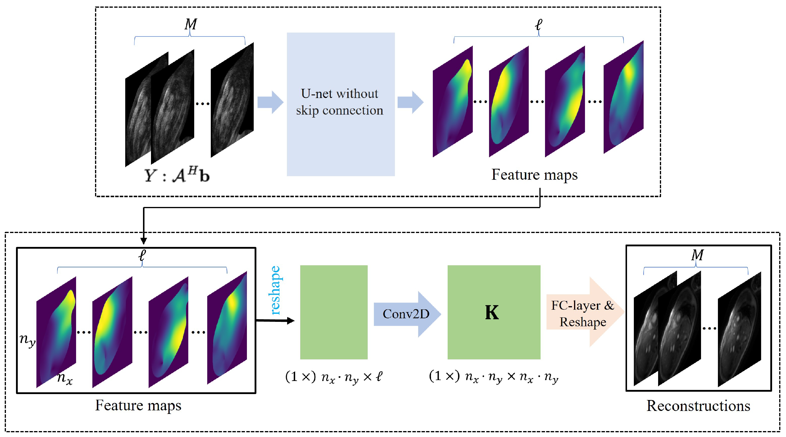
Deep CNN now provides a better way for automatic feature extraction. In this work, we implement the feature extraction operator as a deep CNN with network parameters . We denote the feature extraction network as . The structure of the feature extraction network is illustrated in the upper part of Figure 1.
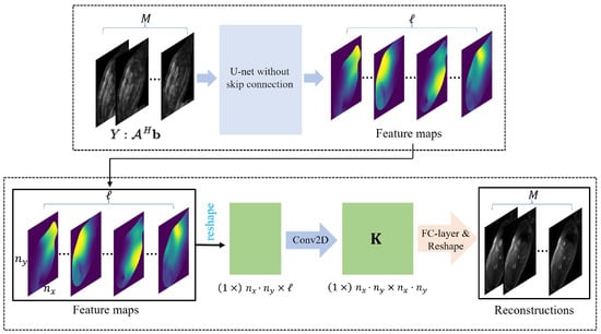
Figure 1.
Illustration of the deep kernel representation. The upper part shows the feature extraction CNN. A U-net without skip connection is used to implement the feature extraction operator in this work. The lower part gives the illustration of the deep kernel representation. The feature maps, which are obtained using the CNN , are first reshaped into the size , where denotes the image size. Then a convolutional layer is used to obtain the kernel matrix . The final reconstructed images in the time series are obtained using a fully-connect (FC) layer and images reshape.
3.2. Deep Kernel Representation
In kernel representation, the choice of the kernel function is important after determining the non-linear feature map. The kernel function is an inner product of the features. Once it is a well-defined inner product, we can get a valid kernel function. In most of the current kernel methods, the kernel functions are chosen empirically. Popular choices of the kernel functions include the radial Gaussian kernel [31]:
and the Dirichlet kernel with bandwidth d [32]:
Besides the empirical choice of the kernel functions, the parameters in the kernel functions, such as in the radial Gaussian kernel and d in the Dirichlet kernel, need manual tuning. This significantly limits the performance of the kernel methods. In this work, we implement the kernel function as a convolutional layer. In other word, we define
where is the intrinsic features in the convolutional layer. is learned directly from the data. We use the word “intrinsic features” to distinguish the features learned from using the feature extraction CNN as described in Section 3.1. The convolution of the feature with the learned intrinsic feature is an inner product [33]. So we have a valid kernel function. The advantage of implementing the kernel function as a convolutional layer is the elimination of the empirical choice of the kernel function and the manual tuning of the kernel parameters. Once we have the kernel matrix with defined as (2), we can have the following image representation:
The multiplication can be implemented using a linear layer and hence can be learned from the data.
With the aforementioned description of kernel representation using CNNs, we can have the following deep kernel representation for the free-breathing and ungated cardiac MRI representation:
Here is the feature extraction network with parameters , is the features in the one-layer CNN for the kernel matrix calculation, and is the parameters in the linear layer. The parameters are learned using back-propagation [34]. The illustration of the deep kernel representation is depicted in Figure 1.
3.3. Free-Breathing and Ungated Cardiac MRI Recovery Using Deep Kernel Representation
With the deep kernel representation, we can use the following minimization criterion to get the parameters , and for free-breathing and ungated cardiac MRI reconstruction:
Here is the total variation regularization, and is chosen to be in this work.
The parameters , and are learned in an unsupervised fashion from only the measured k-t space data of the specific patient. We use ADAM optimization for the learning.
4. Experiments Setup
4.1. Acquisition Scheme and Pre-Processing of Data
In this work, we use the short-axis orientation without a contrast agent to showcase the results. Five subjects were involved in this study, and the public information of these five subjects, including the average heart rate, are shown in Table 1. All the data were acquired on a 3T MR750W scanner (GE Healthcare, Waukesha, WI, USA). The data were acquired using a 2D gradient echo (GRE) sequence with golden angle spiral readouts in a free-breathing and ungated fashion. Some sequence parameters include: FOV = 380 mm × 380 mm; TR = 8 ms; flip angle = 14; slice thickness = 8 mm; readout bandwidth = 500 Hz. The reconstruction matrix size is . All the data was acquired using the AIR coil developed by GE HealthCare (Waukesha, WI, USA). We used an in-house algorithm to pre-select the coils that provide the best signal-to-noise ratio in the region of interest. We then estimated the coil sensitivity maps based on these selected channels using ESPIRiT [35] and assumed them to be constant over time. For each slice, a total number of 950 spirals were acquired. During the reconstruction, the first 200 spirals were deleted. For the rest of the 750 spirals, we bin every five spirals corresponding to 40 ms temporal resolution for each frame in the time series.

Table 1.
Public information of the five subjects involved in this work.
For the comparison purpose, the conventional 2D photoplethysmography (PPG) gated breath-hold images using the balanced steady-state free precession (bSSFP) sequence were also acquired for all the slices. PPG is a simple optical technique used to detect volumetric changes in blood in peripheral circulation and hence can be used as one of the choices for monitoring the cardiac cycle. Balanced steady-state free precession sequence is one type of gradient echo pulse sequence in which a steady, residual transverse magnetization is maintained between successive cycles. For each subject, the breath-hold images of a middle slice were also acquired using a fast gradient echo (FGRE) sequence for comparison. The acquisition scheme for FGRE is Cartesian, while the spiral GRE sequence in the proposed acquisition scheme uses the spiral trajectories, which is non-Cartesian. The parameters for the breath-hold bSSFP sequence were: FOV = 380 mm × 380 mm; spatial resolution = mm × 0.74 mm; TR/TE = 3.5/1.5 ms; flip angle = 49; slice thickness = 8 mm; readout bandwidth = 488 Hz. The parameters for the breath-hold FGRE sequence were: FOV = 380 mm × 380 mm; spatial resolution = mm × 1.48 mm; TR/TE = 5.1/2.8 ms; flip angle = 15; slice thickness = 8 mm; readout bandwidth = 488 Hz.
4.2. State-of-the-Art Method for Comparison
We first compare the reconstructed free-breathing and ungated images with the fully-sampled breath-hold images. Two medical experts were required for consensus scoring for the image quality of the reconstructed free-breathing images and the fully-sampled breath-hold images based on the scoring criteria scales from 1 to 4 (1—non-diagnosable; 2—diagnosable with average image quality; 3—diagnosable with adequate image quality; 4—excellent image quality). Except for the consensus image quality scoring, we also compare the left ventricular ejection fraction (LVEF) and the right ventricular ejection fraction (RVEF) obtained from the breath-hold images and the free-breathing images. The LVEF and RVEF are defined as
Here EDV and ESV denote the end-diastolic volume and end-systolic volume, respectively. We note that in some cases, the basal slices are missing, and the calculated LVEF and RVEF might not represent the accurate LVEF and RVEF of the subjects.
For the reconstruction of free-breathing and ungated cardiac MRI, we compare the proposed deep kernel reconstruction with a state-of-the-art kernel reconstruction method “SToRM”, which was proposed in [18]. The SToRM model exploits the non-linear structure of the dynamic data to estimate the kernel matrix based on a kernel low-rank regularization problem. The kernel matrix is then used to solve the images to be reconstructed. The biggest difference between SToRM and the proposed deep kernel scheme is in the way of calculating the kernel matrix. SToRM relies on a kernel low-rank regularization problem to solve the kernel matrix, while the proposed deep kernel scheme uses CNNs to output the kernel matrix. We note that the SToRM approach yields comparable or improved performance to state-of-the-art self-gated methods.
The quantitative comparisons between the proposed deep kernel method and SToRM are made using the signal-to-noise ratio (SNR) and contrast-to-noise ratio (CNR). We normalize the values for the images for the SNR and CNR calculation. The definitions of SNR and CNR are as follows:
- The SNR is calculated aswhere is the mean intensity value of the user-defined region of interest, and is the standard deviation of the intensity value of a chosen noise region. A higher SNR usually means better image quality. The unit of SNR is dB.
- The CNR is calculated aswhere and are the mean intensity value of two regions within the region of interest and is the standard deviation of the intensity value of a chosen noise region. A higher CNR usually means better image quality. The unit of CNR is dB.
5. Results
5.1. Free-Breathing and Ungated Cardiac MRI Using Deep Kernel Method
We use the proposed deep kernel method to reconstruct the free-breathing and ungated cardiac MRI. The method was implemented using the PyTorch library. The GPU acceleration of the non-uniform FFT and non-uniform IFFT was realized using the TorchKbNufft package [36]. The reconstructions were run on a machine with an Intel Xeon CPU at 2.40 GHz and a Tesla V100 32 GB GPU.
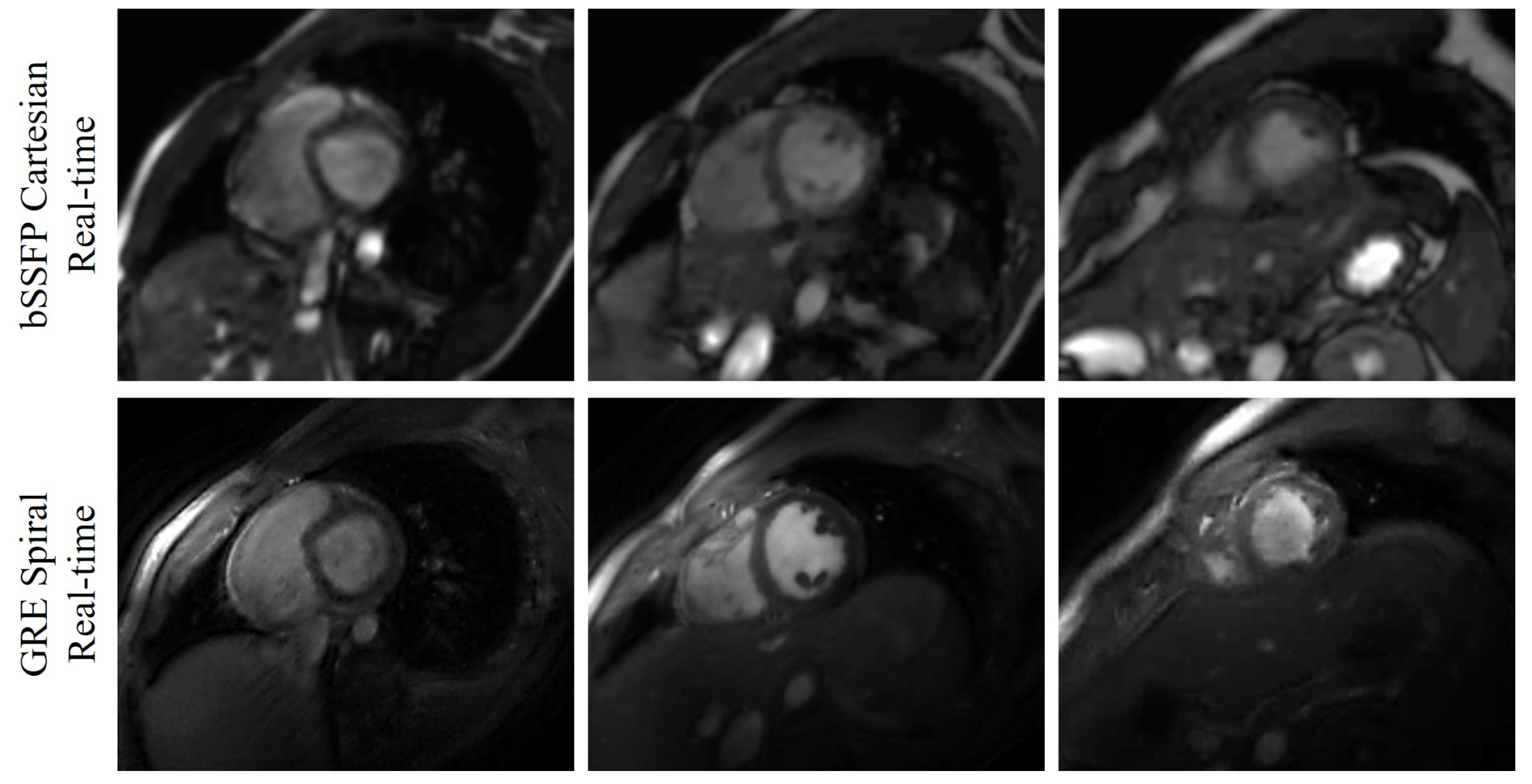
The output of each image has two channels, which correspond to the real and imaginary parts of the MR image. For the convolutional layers which have activation functions, we use Leaky ReLU with slope 0.2. Thirty-seven slices from five subjects were reconstructed in this work. Among the five subjects, we collected the basal slices for two subjects. The deep kernel method is also able to reconstruct the basal slices. The reconstructions of eight slices from Subject #2 were shown in Figure 2. We have also shown the comparison between the bSSFP Cartesian real-time images with acceleration factor 5 and the GRE spiral real-time images reconstructed using the deep kernel method in Figure 3.

Figure 2.
Showcase of the reconstruction of free-breathing and ungated cardiac MRI using the proposed deep kernel method. The eight slices are from Subject #2. The first row shows the end-diastolic phase, and the second row is the end-systolic phase.
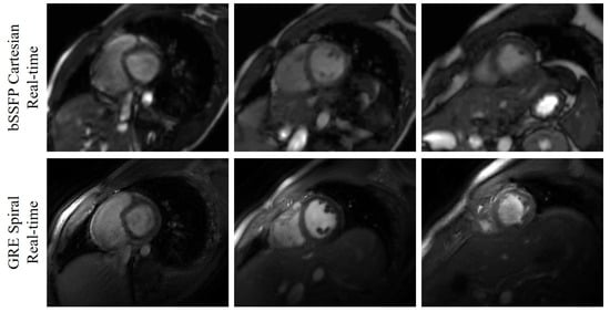
Figure 3.
Comparison between the bSSFP Cartesian real-time images with acceleration factor 5 and the GRE spiral real-time images reconstructed using the deep kernel method. The three slices (one basal slice, one mid slice, and one apex slice) are from Subject #3. The first row shows the bSSFP Cartesian real-time images, and the second row is the GRE spiral real-time images.
5.2. Comparisons with Fully-Sampled Breath-Hold Images
In this section, we show the results of the comparison between the reconstructed free-breathing images and the fully-sampled breath-hold images.
For the data acquisition, except for the highly undersampled k-space data for all the slices from the five subjects, we also acquired the fully-sampled breath-hold data for all the corresponding slices using the clinical bSSFP sequence. Moreover, we also acquired the fully-sampled breath-hold images for one middle slice for each subject using the commercial FGRE sequence.
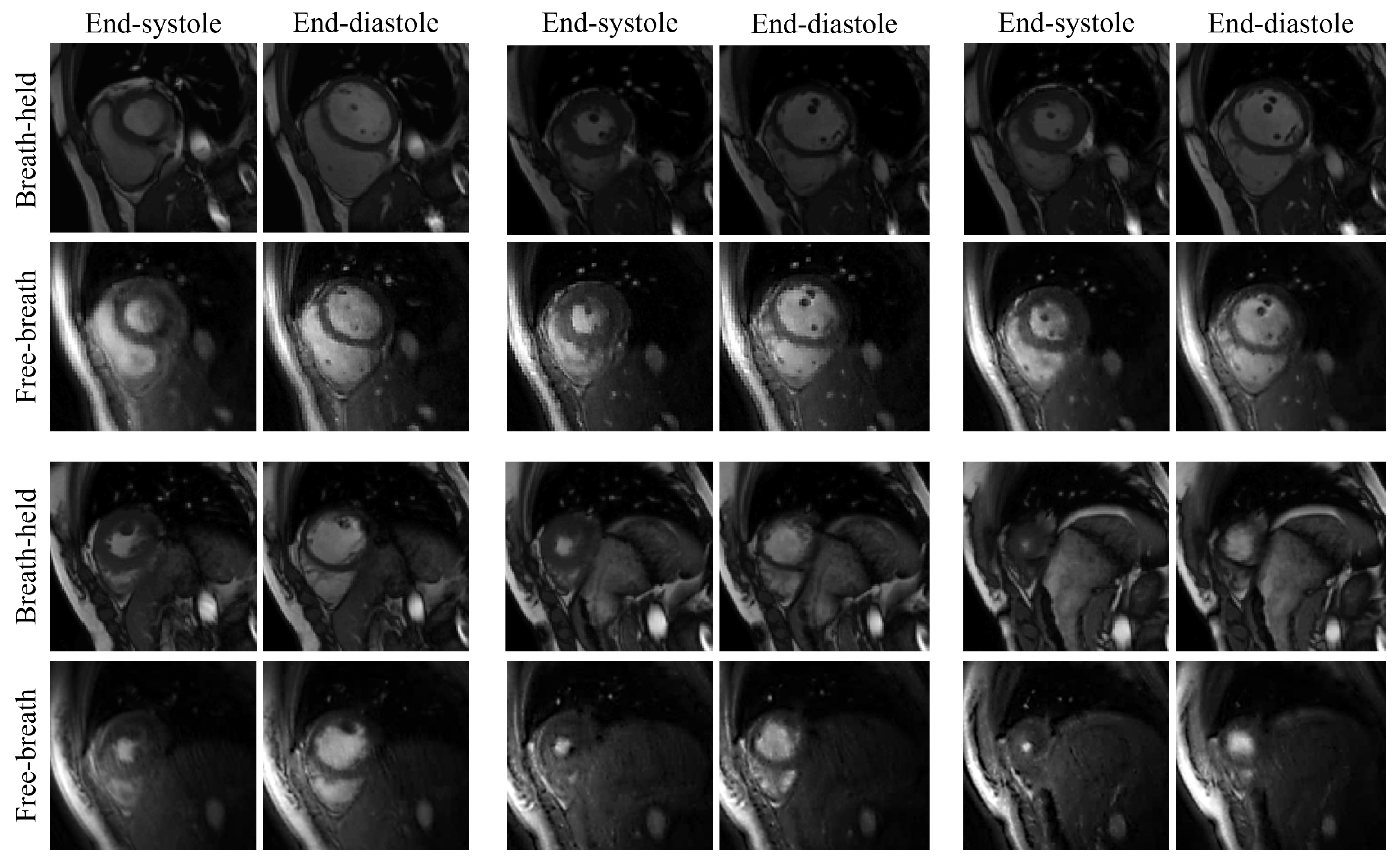
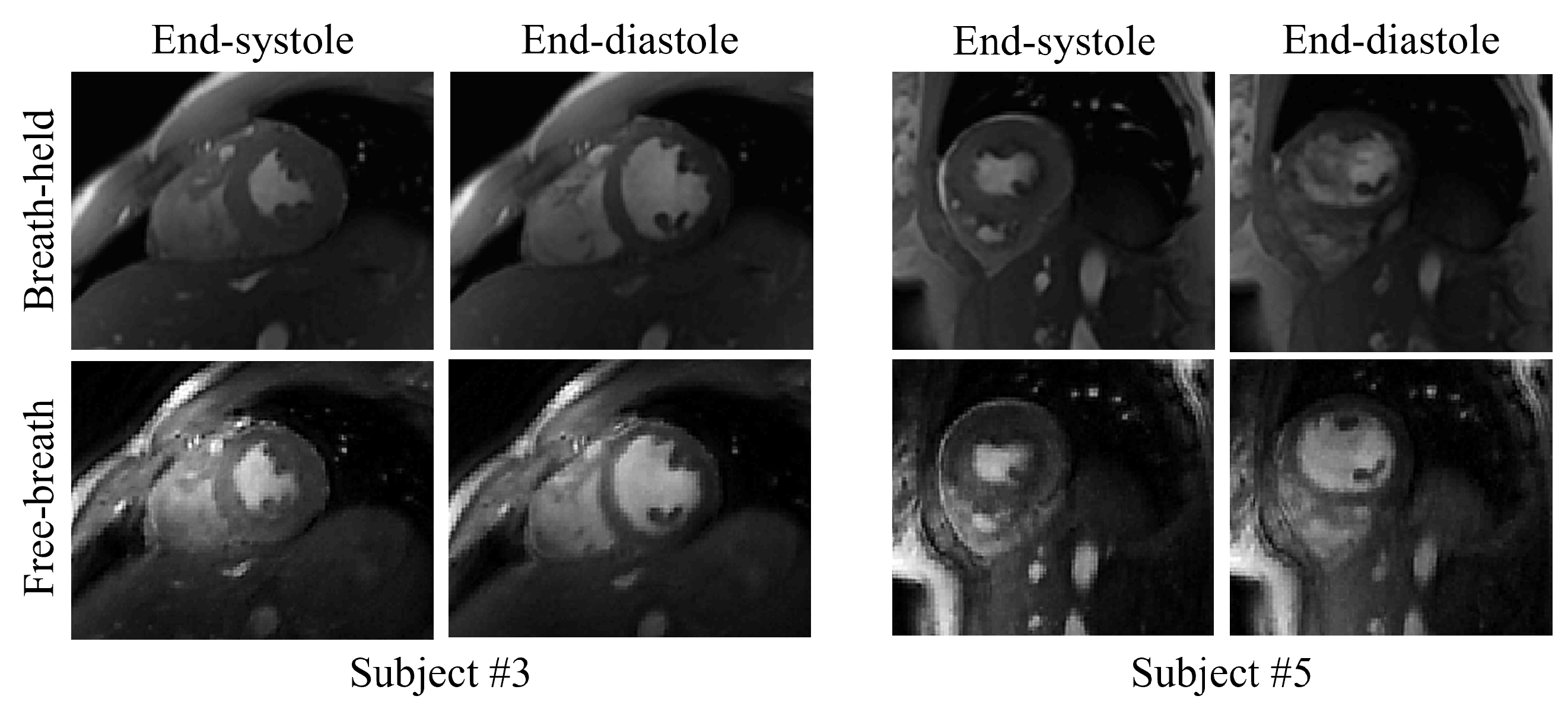
In Figure 4, we showed the visual comparison of the reconstructed free-breathing images and the fully-sampled breath-hold images acquired using the bSSFP sequence. The slices shown in Figure 4 were from Subject #4. Figure 5 was the visual comparison of the reconstructed free-breathing images and the fully-sampled breath-hold images acquired using the FGRE sequence. We reconstructed the whole time series, and we randomly chose a cardiac cycle (from end-systolic to end-diastolic) for comparison with the breath-hold cine.
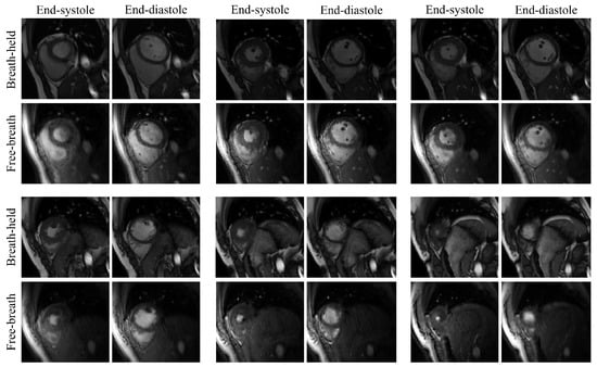
Figure 4.
Visual comparison of the reconstructed free-breathing images and the fully-sampled breath-hold images. End-systolic and end-diastolic phases from six slices are shown in the figure. The six slices are from Subject #4. We note that the free-breathing images are acquired using the GRE sequence and the fully-sampled breath-hold images are acquired using the bSSFP sequence. This results in different contrast between the two types of the images.
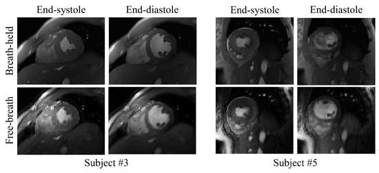
Figure 5.
Visual comparison of the reconstructed free-breathing images and the fully-sampled breath-hold images acquired using FGRE sequence. For each subject, we acquired fully-sampled breath-hold images for one middle slice using the FGRE sequence. End-systolic and end-diastolic phases from two slices from two subjects are shown in the figure.
Quantitative comparisons between the free-breathing images and the breath-hold images were performed based on image quality assessment by experts, LVEF, and RVEF.
Figure 6 showed the results of consensus image quality scoring done in a blinded fashion by two medical experts. From the scores, we can see that the fully-sampled breath-hold images acquired using the bSSFP have the highest image quality. While we do not see a big difference in the image quality for the free-breathing images and the fully-sampled breath-hold images acquired using the FGRE sequence (average score of 2.8 and 2.9, respectively).
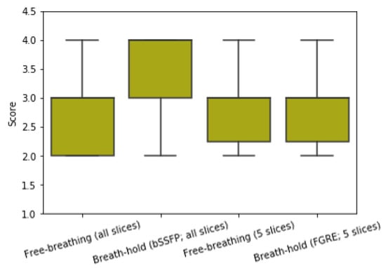
Figure 6.
Comparison of image quality of the free-breathing images and breath-hold images. Image quality assessment is done in a blinded fashion by two medical experts. We reconstructed all the short-axis slices acquired from five subjects. We also acquired the fully-sampled breath-hold images for all the slices using the bSSFP sequence. For each subject, we scanned one middle slice using the product FGRE sequence provided by GE HealthCare. The free-breathing images from all the slices received an average score of 2.7, and the clinical fully-sampled images using the bSSFP sequence got an average score of 3.6. The fully-sampled breath-hold images acquired using the FGRE sequence received an average score of 2.9, and the free-breathing images corresponding to these five slices got an average score of 2.8. From which we can see that the reconstructed free-breathing images have similar image quality as the fully-sampled breath-hold images acquired using the product FGRE sequence, even though the images were highly undersampled and acquired in a free-breathing and ungated fashion.
Table 2 gave the results of the LVEF and RVEF comparison. The LVEF and RVEF calculations for the fully-sampled images were done using commercial software (Circle cv42, Calgary, AB, Canada). Automatic segmentation was first performed for the fully-sampled images using the software, and we then manually corrected the segmentation. The LVEF and RVEF calculations for the free-breathing images were done using Matlab 2019a. We manually drew the contours for the free-breathing images to calculate the EF. Since bulk motions were involved in the data acquisition for Subject #1 and we did not have exactly matching breath-hold and free-breathing slices. Hence we skipped Subject #1 for LVEF and RVEF comparison. We also reported the corresponding left ventricular end-diastolic volume (LVEDV), left ventricular end-systolic volume (LVESV), right ventricular end-diastolic volume (RVEDV), and right ventricular end-systolic volume (RVESV). From the statistical analysis, we can see that there is no significant difference between the LVEF and RVEF obtained from the fully-sampled breath-hold images and the highly undersampled free-breathing images.

Table 2.
LVEF and RVEF comparison. Since bulk motions were introduced during the data acquisition of subject #1 and we do not have the matching breath-hold and free-breathing slices for this subject. Therefore, the LVEF and RVEF are compared based on only four subjects. The LVEF calculated from the free-breathing and ungated images and the LVEF calculated from the fully-sampled breath-hold images have a p-value of . The RVEF calculated from the free-breathing and ungated images and the RVEF calculated from the fully-sampled breath-hold images have a p-value of . The p-values indicate that the LVEF and RVEF got from the free-breathing images and breath-hold images have no significant difference.
5.3. Comparisons with Current Kernel Method
In this part, we compare the reconstructed images using both the proposed deep kernel method and the SToRM method, which is a state-of-the-art kernel method.
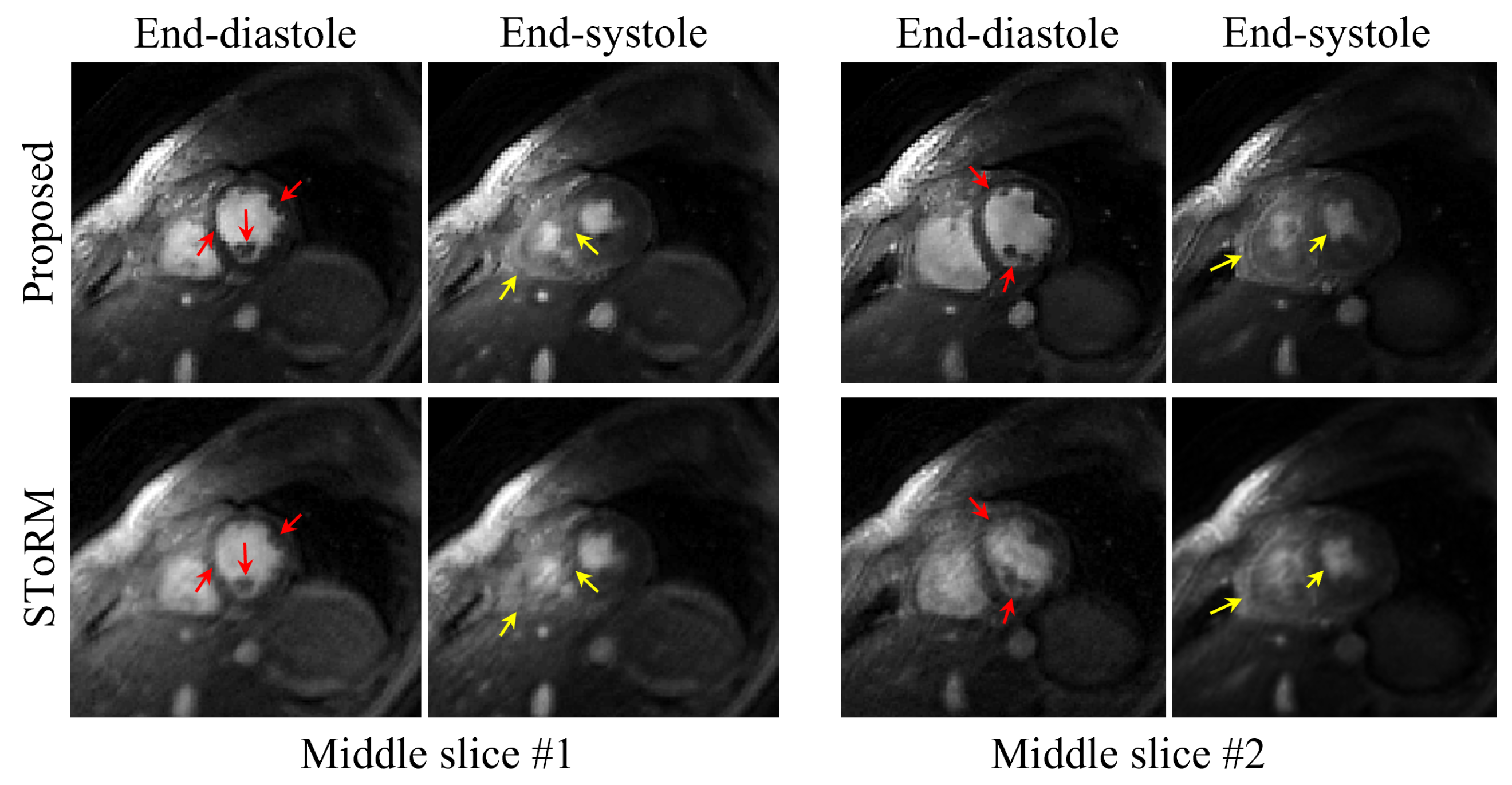
Figure 7 showed the visual comparison of the reconstructed images using the two methods. The end-diastolic and the end-systolic phases from two slices were shown in the figure. From the figures, we can see that the proposed deep kernel scheme can reduce the blurring and the motion artifacts in the reconstructed images compared to the images obtained from the SToRM method. This enables us to see more heart details in the reconstructed images. For example, we can see the papillary muscles and the RV free-wall more clearly in the reconstructed images using the deep kernel method.
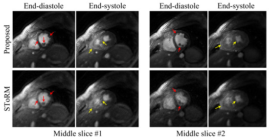
Figure 7.
Comparison of the reconstructions from the proposed method and the SToRM method. We showed the end-diastolic and end-systolic phases from two slices acquired from Subject #1. From the images, we can see that the proposed reconstruction scheme can provide images with sharper edges, and the papillary muscles are more visible (illustrated by the red arrows in the images). Furthermore, from the end-systolic images, we can see that the proposed scheme provides reduced motion artifacts, and the RV free-wall is more clear (illustrated by the yellow arrows in the images).
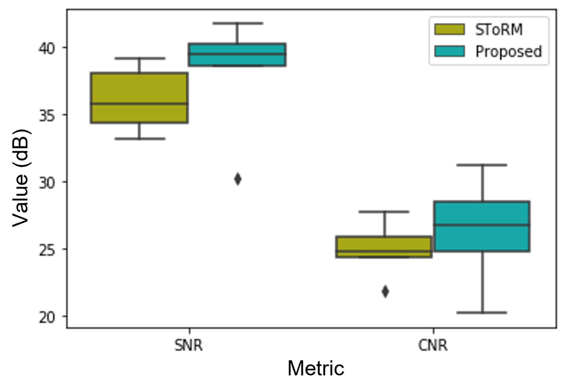
The improved image quality from the proposed method was also confirmed by the quantitative results, which were shown in Figure 8. The SNR and CNR calculations were done using Matlab 2019a. We manually chose the regions (region of interest and the noise region) for the calculation. For the SNR calculation, we choose a square region in the left ventricle as the region of interest and a square region out of the body as the noise region. For the CNR calculation, we choose two square regions in the left ventricle as the regions of interest and a square region out of the body as the noise region. From the quantitative results, we can see that the reconstruction from the proposed method can provide about 2 dB improvement in SNR and about 1.5 dB improvement in CNR compared to the competing SToRM method.
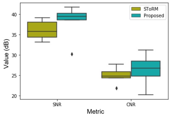
Figure 8.
SNR and CNR comparison of the images reconstructed from the proposed scheme and the SToRM method. The average SNR and CNR of the images reconstructed from the proposed method are 37.99 dB and 26.28 dB. While the average SNR and CNR of the images reconstructed from SToRM are 36.01 dB and 24.89 dB. From the quantitative comparison, we can see that the proposed deep kernel method can provide improved image quality compared to the existing kernel method.
6. Discussion
In this work, we proposed a deep kernel method for the reconstruction of free-breathing and ungated cardiac MRI. A GRE sequence with spiral readouts is implemented to acquire the highly undersampled free-breathing and ungated data.
The non-Cartesian spiral k-space trajectories with golden angle increment are used for data acquisition because it is more robust to motion effects compared to the Cartesian acquisition. Furthermore, the long spiral trajectories enable more data samples in the center k-space region, and the longer repetition time from the spiral trajectories offers enhanced inflow contrast between the myocardium and blood pool. Another advantage of the spiral trajectories is that they are less sensitive to the eddy-current effects compared to other non-Cartesian trajectories, such as radial trajectories. Hence we did not perform k-space trajectories correction in this work. In addition to the spiral k-space trajectories, the spoiled GRE sequence for the data acquisition in this work does not suffer from banding artifacts, which are usually seen in the images acquired using the bSSFP sequence without shimming.
Even the spiral GRE sequence has a few advantages, we can see from the image quality assessment done by experts that the images acquired from the bSSFP sequence have the best image quality. Indeed, the bSSFP sequence is widely used in clinical cardiac MRI due to the short acquisition time and high contrast between the blood pool and myocardium. So one direction in the future is to design a better non-Cartesian sequence based on the bSSFP sequence for free-breathing and ungated cardiac MRI to get further improved image quality with even shorter acquisition time.
Five volunteers were recruited for this study: three of them are healthy volunteers, and two of them have heart problems. In the future, we plan to have more subjects with different health conditions to study the feasibility of real-time free-breathing and ungated cardiac MRI using the proposed deep kernel framework.
We demonstrate the deep kernel framework in free-breathing and ungated real-time cardiac MRI reconstruction. We note that we may also apply the framework to free-breathing and ungated first-pass perfusion, mapping, mapping, and late gadolinium enhancement imaging. We will investigate the application of the deep kernel method in different applications in the future work.
7. Conclusions
In this work, a deep kernel method was introduced for real-time free-breathing and ungated cardiac MRI reconstruction. We implemented the deep kernel method using a cascade of two CNNs. We realized the feature extraction operator using a deep CNN, and a one-layer CNN is used for the kernel matrix calculation. The benefits of the proposed deep kernel methods are the elimination of the manual choices for the feature map and the kernel function, as well as the elimination of the manual tuning of the parameters in the kernel functions in the traditional kernel methods. This results in the improved performance of the deep kernel method. Moreover, the proposed scheme is unsupervised, which ideally fits the settings of free-breathing dynamic MRI. Comparisons with the competing state-of-the-art kernel method show improved reconstructions using the proposed deep kernel method.
Author Contributions
Methodology: Q.Z.; data acquisition: Q.Z. and A.H.A.; images rating: S.D. and T.H.; statistical analysis: Q.Z. and T.H.; writing—original draft preparation: Q.Z. and T.H.; writing—review and editing: Q.Z., S.D. and T.H. All authors have read and agreed to the published version of the manuscript.
Funding
This work was conducted on an MRI instrument funded by NIH 1S10OD025025-01.
Institutional Review Board Statement
The Institutional Review Board at the University of Iowa approved the acquisition of the data.
Informed Consent Statement
Informed consent was obtained from all subjects involved in the study.
Data Availability Statement
The data presented in this study are available on request from the corresponding author. The data has not been made publicly available due to the confidentiality of the data.
Acknowledgments
Q.Z. would like to thank the Magnetic Resonance Research Facility (MRRF) at the University of Iowa for providing the resources for data acquisition, and the University of Iowa Research Services for providing the GPU and HPC resources for running the experiments.
Conflicts of Interest
The authors declare no conflict of interest.
References
- Lustig, M.; Donoho, D.; Pauly, J.M. Sparse MRI: The application of compressed sensing for rapid MR imaging. Magn. Reson. Med. 2007, 58, 1182–1195. [Google Scholar] [CrossRef]
- Lustig, M.; Donoho, D.L.; Santos, J.M.; Pauly, J.M. Compressed sensing MRI. IEEE Signal Process. Mag. 2008, 25, 72–82. [Google Scholar] [CrossRef]
- Gamper, U.; Boesiger, P.; Kozerke, S. Compressed sensing in dynamic MRI. Magn. Reson. Med. 2008, 59, 365–373. [Google Scholar] [CrossRef] [PubMed]
- Haldar, J.P.; Hernando, D.; Liang, Z.P. Compressed-sensing MRI with random encoding. IEEE Trans. Med. Imaging 2010, 30, 893–903. [Google Scholar] [CrossRef] [PubMed]
- Deshmane, A.; Gulani, V.; Griswold, M.A.; Seiberlich, N. Parallel MR imaging. J. Magn. Reson. Imaging 2012, 36, 55–72. [Google Scholar] [CrossRef] [PubMed]
- Niendorf, T.; Sodickson, D.K. Parallel imaging in cardiovascular MRI: Methods and applications. NMR Biomed. 2006, 19, 325–341. [Google Scholar] [CrossRef]
- Baert, A. Parallel Imaging in Clinical MR Applications; Springer: Berlin/Heidelberg, Germany, 2007. [Google Scholar]
- Qin, C.; Schlemper, J.; Caballero, J.; Price, A.N.; Hajnal, J.V.; Rueckert, D. Convolutional recurrent neural networks for dynamic MR image reconstruction. IEEE Trans. Med. Imaging 2018, 38, 280–290. [Google Scholar] [CrossRef]
- Küstner, T.; Fuin, N.; Hammernik, K.; Bustin, A.; Qi, H.; Hajhosseiny, R.; Masci, P.G.; Neji, R.; Rueckert, D.; Botnar, R.M.; et al. CINENet: Deep learning-based 3D cardiac CINE MRI reconstruction with multi-coil complex-valued 4D spatio-temporal convolutions. Sci. Rep. 2020, 10, 13710. [Google Scholar] [CrossRef]
- Sandino, C.M.; Lai, P.; Vasanawala, S.S.; Cheng, J.Y. Accelerating cardiac cine MRI using a deep learning-based ESPIRiT reconstruction. Magn. Reson. Med. 2021, 85, 152–167. [Google Scholar] [CrossRef]
- Feng, L.; Grimm, R.; Block, K.T.; Chandarana, H.; Kim, S.; Xu, J.; Axel, L.; Sodickson, D.K.; Otazo, R. Golden-angle radial sparse parallel MRI: Combination of compressed sensing, parallel imaging, and golden-angle radial sampling for fast and flexible dynamic volumetric MRI. Magn. Reson. Med. 2014, 72, 707–717. [Google Scholar] [CrossRef]
- Feng, L.; Axel, L.; Chandarana, H.; Block, K.T.; Sodickson, D.K.; Otazo, R. XD-GRASP: Golden-angle radial MRI with reconstruction of extra motion-state dimensions using compressed sensing. Magn. Reson. Med. 2016, 75, 775–788. [Google Scholar] [CrossRef]
- Deng, Z.; Pang, J.; Yang, W.; Yue, Y.; Sharif, B.; Tuli, R.; Li, D.; Fraass, B.; Fan, Z. Four-dimensional MRI using three-dimensional radial sampling with respiratory self-gating to characterize temporal phase-resolved respiratory motion in the abdomen. Magn. Reson. Med. 2016, 75, 1574–1585. [Google Scholar] [CrossRef] [PubMed]
- Usman, M.; Atkinson, D.; Kolbitsch, C.; Schaeffter, T.; Prieto, C. Manifold learning based ECG-free free-breathing cardiac CINE MRI. J. Magn. Reson. Imaging 2015, 41, 1521–1527. [Google Scholar] [CrossRef] [PubMed]
- Shetty, G.N.; Slavakis, K.; Bose, A.; Nakarmi, U.; Scutari, G.; Ying, L. Bi-linear modeling of data manifolds for dynamic-MRI recovery. IEEE Trans. Med. Imaging 2019, 39, 688–702. [Google Scholar] [CrossRef]
- Zou, Q.; Ahmed, A.H.; Nagpal, P.; Kruger, S.; Jacob, M. Dynamic imaging using a deep generative SToRM (Gen-SToRM) model. IEEE Trans. Med. Imaging 2021, 40, 3102–3112. [Google Scholar] [CrossRef] [PubMed]
- Zou, Q.; Ahmed, A.H.; Nagpal, P.; Priya, S.; Schulte, R.F.; Jacob, M. Variational manifold learning from incomplete data: Application to multi-slice dynamic MRI. IEEE Trans. Med. Imaging 2022, 41, 3552–3561. [Google Scholar] [CrossRef] [PubMed]
- Ahmed, A.H.; Zhou, R.; Yang, Y.; Nagpal, P.; Salerno, M.; Jacob, M. Free-breathing and ungated dynamic mri using navigator-less spiral storm. IEEE Trans. Med. Imaging 2020, 39, 3933–3943. [Google Scholar] [CrossRef] [PubMed]
- Schölkopf, B.; Smola, A.J.; Bach, F. Learning with Kernels: Support Vector Machines, Regularization, Optimization, and Beyond; MIT Press: Cambridge, MA, USA, 2002. [Google Scholar]
- Nakarmi, U.; Wang, Y.; Lyu, J.; Liang, D.; Ying, L. A kernel-based low-rank (KLR) model for low-dimensional manifold recovery in highly accelerated dynamic MRI. IEEE Trans. Med. Imaging 2017, 36, 2297–2307. [Google Scholar] [CrossRef]
- Poddar, S.; Jacob, M. Recovery of noisy points on bandlimited surfaces: Kernel methods re-explained. In Proceedings of the 2018 IEEE International Conference on Acoustics, Speech and Signal Processing (ICASSP), Calgary, AB, Canada, 15–20 April 2018; IEEE: Piscataway, NJ, USA, 2018; pp. 4024–4028. [Google Scholar]
- Arif, O.; Afzal, H.; Abbas, H.; Amjad, M.F.; Wan, J.; Nawaz, R. Accelerated dynamic MRI using kernel-based low rank constraint. J. Med. Syst. 2019, 43, 271. [Google Scholar] [CrossRef]
- Garcia-Gasulla, D.; Parés, F.; Vilalta, A.; Moreno, J.; Ayguadé, E.; Labarta, J.; Cortés, U.; Suzumura, T. On the behavior of convolutional nets for feature extraction. J. Artif. Intell. Res. 2018, 61, 563–592. [Google Scholar] [CrossRef]
- Han, Y.; Yoo, J.; Kim, H.H.; Shin, H.J.; Sung, K.; Ye, J.C. Deep learning with domain adaptation for accelerated projection-reconstruction MR. Magn. Reson. Med. 2018, 80, 1189–1205. [Google Scholar] [CrossRef] [PubMed]
- Aggarwal, H.K.; Mani, M.P.; Jacob, M. MoDL: Model-based deep learning architecture for inverse problems. IEEE Trans. Med Imaging 2018, 38, 394–405. [Google Scholar] [CrossRef] [PubMed]
- Lee, D.; Yoo, J.; Tak, S.; Ye, J.C. Deep residual learning for accelerated MRI using magnitude and phase networks. IEEE Trans. Biomed. Eng. 2018, 65, 1985–1995. [Google Scholar] [CrossRef]
- Li, Z.; Li, C. Selection of kernel function for least squares support vector machines in downburst wind speed forecasting. In Proceedings of the 2018 11th International Symposium on Computational Intelligence and Design (ISCID), Hangzhou, China, 8–9 December 2018; IEEE: Piscataway, NJ, USA, 2018; Volume 2, pp. 337–341. [Google Scholar]
- Dunteman, G.H. Principal Components Analysis; Sage: Southend Oaks, CA, USA, 1989. [Google Scholar]
- Stone, J.V. Independent Component Analysis: A Tutorial Introduction; MIT Press: Cambridge, MA, USA, 2004. [Google Scholar]
- Van der Maaten, L.; Hinton, G. Visualizing data using t-SNE. J. Mach. Learn. Res. 2008, 9, 2579–2605. [Google Scholar]
- Fasshauer, G.E.; McCourt, M.J. Stable evaluation of Gaussian radial basis function interpolants. SIAM J. Sci. Comput. 2012, 34, A737–A762. [Google Scholar] [CrossRef]
- Zou, Q.; Jacob, M. Recovery of surfaces and functions in high dimensions: Sampling theory and links to neural networks. SIAM J. Imaging Sci. 2021, 14, 580–619. [Google Scholar] [CrossRef]
- Ramachandran, P.; Parmar, N.; Vaswani, A.; Bello, I.; Levskaya, A.; Shlens, J. Stand-alone self-attention in vision models. Adv. Neural Inf. Process. Syst. 2019, 32. [Google Scholar]
- LeCun, Y.; Touresky, D.; Hinton, G.; Sejnowski, T. A theoretical framework for back-propagation. In Proceedings of the 1988 Connectionist Models Summer School, Pittsburgh, PA, USA, 17–26 June 1988; Volume 1, pp. 21–28. [Google Scholar]
- Uecker, M.; Lai, P.; Murphy, M.J.; Virtue, P.; Elad, M.; Pauly, J.M.; Vasanawala, S.S.; Lustig, M. ESPIRiT—An eigenvalue approach to autocalibrating parallel MRI: Where SENSE meets GRAPPA. Magn. Reson. Med. 2014, 71, 990–1001. [Google Scholar] [CrossRef]
- Muckley, M.J.; Stern, R.; Murrell, T.; Knoll, F. TorchKbNufft: A high-level, hardware-agnostic non-uniform fast Fourier transform. In Proceedings of the ISMRM Workshop on Data Sampling & Image Reconstruction, Sedona, AZ, USA, 26–29 January 2020. [Google Scholar]
Disclaimer/Publisher’s Note: The statements, opinions and data contained in all publications are solely those of the individual author(s) and contributor(s) and not of MDPI and/or the editor(s). MDPI and/or the editor(s) disclaim responsibility for any injury to people or property resulting from any ideas, methods, instructions or products referred to in the content. |
© 2023 by the authors. Licensee MDPI, Basel, Switzerland. This article is an open access article distributed under the terms and conditions of the Creative Commons Attribution (CC BY) license (https://creativecommons.org/licenses/by/4.0/).

