Abstract
Vulnerability prediction, in which static analysis is leveraged to predict the vulnerabilities of binary programs, has become a popular research topic. Traditional vulnerability prediction methods depend on vulnerability patterns, which must be predefined by security experts in a time-consuming manner. The development of Artificial Intelligence (AI) has yielded new options for vulnerability prediction. Neural networks allow vulnerability patterns to be learned automatically. However, current works extract only one or two types of features and use traditional models such as word2vec, which results in the loss of much instruction-level information. In this paper, we propose a model named SAViP to predict vulnerabilities in binary programs. To fully extract binary information, we integrate three kinds of features: semantic, statistical, and structural features. For semantic features, we apply the Masked Language Model (MLM) pre-training task of the RoBERTa model to the assembly code to build our language model. Using this model, we innovatively combine the beginning token and the operation-code token to create the instruction embedding. For the statistical features, we design a 56-dimensional feature vector that contains 43 kinds of instructions. For the structural features, we improve the ability of the structure2vec network to obtain the characteristic of the network by emphasizing node self-attention. Through these optimizations, we significantly increase the accuracy of vulnerability prediction over existing methods. Our experiments show that SAViP achieves a recall of 77.85% and Top 100∼600 accuracies all above 95%. The results are 10% and 13% higher than those of the state-of-the-art V-Fuzz, respectively.
1. Introduction
The static analysis of binary programs is an important part of software security research. While dynamic analysis methods need to execute the program repeatedly, static methods can directly run security detection without executing the program, consequently resulting in lower computational costs and time consumption. Moreover, while dynamic methods are limited to only conducting security detection on executed running paths, static methods are more comprehensive and consider the whole program.
Vulnerability prediction, in which static analysis is leveraged to predict program vulnerabilities, is an important component in software security testing. By doing predictions, researchers can analyze the weakness of programs. In addition, a successful prediction model can accelerate dynamic analysis. For example, the vulnerability prediction model can be regarded as a better standard to choose seeds for directed fuzzer, which emphasizes the most vulnerable part of programs and avoids useless time costs. However, traditional static analysis is limited in a number of ways. Most methods of static analysis depend on the definition of vulnerability patterns by security experts, which can be tedious and time-consuming. Since these patterns are typically manually defined, it can be difficult to automate this process, further leading to difficulty in applying it in large-scale programs. Moreover, many static analysis tools [1,2] are designed for source codes in specific languages; for example, Reshift [3] only detects vulnerabilities for JAVA programs.
Considering these shortages, some researchers attempt to apply neural networks in detecting vulnerabilities [4,5,6,7,8,9,10] for the following reasons. First, with a large number of samples, the vulnerability patterns can be learned automatically by neural networks. Second, neural networks can identify the deep, complicated features of programs, which can be difficult to define as patterns even by experts. In addition, multiple types of vulnerabilities can be detected simultaneously by neural network approaches. In contrast, only one specific type of vulnerability can be detected once by using pattern-based methods.
However, current methods using neural networks in vulnerability prediction still have limitations. P1: Most neural networks are designed to detect vulnerabilities in source codes [4,5,6]. However, many software programs only provide binary files, which have no source code available for security analysis [7]. This makes current methods difficult to apply in actual software security testing. P2: The current methods lack effective semantic features. The features of programs can be divided into three dimensions, semantic, statistical, and structural features. However, existing binary-based methods extract only one or two types of features, and most [11] only focus on semantic and structural features. V-Fuzz [12] considers the value of statistical characteristics, but it lacks the ability to extract semantic features. Moreover, it counts the respective quantities of all instructions, which is redundant and results in an increase in overhead. In addition, it should be noticed that most works [8,11] extract semantic features by utilizing word2vec [13], which only produces word embeddings and leads to the loss of instruction-level information.
To address the aforementioned problems, we propose SAViP, a semantic-aware model for vulnerability prediction in binary programs. As shown in Figure 1, we first disassemble the binary programs and represent an assembly language-based function as a control flow graph (CFG). Then, covert the CFG to an attributed control flow graph (ACFG) and generate the function embedding. Finally, we make predictions in the light of the embeddings. Overall, SAViP consists of three parts that separately model the semantic, statistical, and structural features of binary programs.
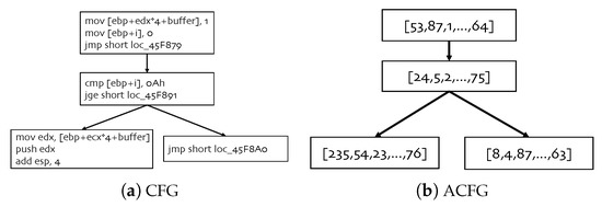
Figure 1.
Two types of representation graphs for binary programs. CFG is the control flow graph for assembly functions. ACFG is the vectorization of CFG. Each basic block in ACFG corresponds to a feature vector of the CFG block.
For the semantic features, we introduce the pre-training task of the advanced natural language process (NLP) model RoBERTa [14] for assembly programs. We first use a dynamic masking task in assembly files to learn better representations of the instructions. We then employ the pre-trained model to extract the semantic features for each instruction. Considering that the operation code plays an essential role in the semantics of each assembly instruction, we propose using a combination of the final hidden vectors of the beginning token and the operation-code token. This design not only considers the entire instructions but also places greater emphasis on the operation code. For the statistical features, we design a 56-dimensional feature vector that contains 43 instructions. To reduce the dimensionality of the statistical features, we choose only four types of instructions [15]: data transfer, binary arithmetic, logical, and control transfer instructions. Our experiment shows that these instructions contain most of the information regarding vulnerabilities. To combine the structural features, i.e., the CFG of a given function, and the other two types of features together, we utilize the ACFG [16] as the intermediate representation. Each node in the ACFG is the concatenated block vector of the corresponding semantic feature and statistical feature. We finally improve the structure2vec [17] network by emphasizing node self-attention. Through our designed graph neural network, each block node from a given assembly function can fuse the information of its neighbors and learn the features of the whole assembly function.
We conduct experiments on Juliet Test Suite v1.3 [18], a dataset that has been widely used in vulnerability related works. Our proposed SAViP achieves a recall of 77.85% and Top 100∼600 accuracies above 95%, which are 10 percentage points and 13 percentage points, respectively, higher than those of the state-of-the-art V-fuzz model. We also determine the best parameters that can balance model performance and time consumption through comparative experiments. Moreover, our ablation study shows that the semantic features contribute the most to the performance of SAViP.
In summary, our work makes the following contributions:
- We propose SAViP, a semantic-aware model for vulnerability prediction that utilizes the semantic, statistical, and structural features of binary programs.
- To better extract semantic information from instructions, we introduce the pre-training task of the RoBERTa model to assembly language and further employ the pre-trained model to generate semantic embeddings for the instructions.
- Experiments show that our SAViP makes significant improvements over the previous state-of-the-art V-fuzz (recall +10%) and achieves new state-of-the-art results for vulnerability prediction.
2. Related Work
2.1. Vulnerability Prediction
Vulnerability prediction is an important research direction in software security. Traditional solutions use pattern-based methods, whose vulnerability patterns are defined prior to detection. However, these methods are inefficient and have weak scalability. Recently, deep learning methods have proven to be useful in this area, but as with traditional methods, there are some shortcomings in current approaches. First, most of the works are based on source code [5,6,19], while in reality, application software is often closed source, and acquisition of the source code can be difficult. Second, binary-based methods always lack information and tend to be highly time-consuming.
A typical deep learning-based method [8] uses LLVM IR [20] and word2vec for word embeddings. This method merges the word vectors in the function into an array and uses a recurrent neural network (RNN) [21] for classification. However, the word2vec model is a word embedding model; it cannot be used to discover the internal features at the instruction level. Moreover, the model ignores statistical and structural features, and only shallow semantic features are considered. The use of RNN also greatly increases the time costs of model training and requires stronger hardware support. BVDetector [11] improves upon this method by adding data flow and control flow analysis but still depends on the word2vec model and RNN [22]. Furthermore, the method [8] and BVDetector [11] lack positional information when extracting semantic features, while the positions of instructions are important to instruction semantics. SAViP uses RoBERTa [14], a state-of-the-art NLP model, to extract semantic features, which combines instruction semantics and positional information and makes generated embeddings more comprehensive.
V-Fuzz [12] introduces the importance of prediction scores; by outputting the vulnerability probabilities of functions, it speeds up dynamic analysis [23,24,25]. The prediction model of V-Fuzz uses structural and statistical features and obtains prediction scores through a graph embedding network. The information from binary programs is retained to a large extent with this design; however, the semantic features are totally ignored, which makes V-Fuzz less robust against vulnerability variants. Moreover, V-Fuzz counts all of the instructions of the x86 architecture, which creates an over-redundant feature vector.
2.2. Intermediate Representation
To analyze a binary program, it is necessary to use an appropriate form of representation, that is, to convert the program into a form that is suitable for analysis. We can concatenate all the basic blocks of a function to obtain its word vector array (as described in [8]). However, this completely ignores the internal structure of the function and easily leads to a vector with excessively high dimensionality. Considering that we need to combine semantic features, statistical features, and structural features, our model uses the ACFG [16] as the intermediate representation of the function.
The ACFG is the vectorization of the CFG. Given the CFG of a function, as shown in Figure 1a, if we obtain the vector representation of each basic block, we can use this set of vectors to replace the basic block. The new graph obtained in this way, as shown in Figure 1b, is called the ACFG. Although the ACFG vectorizes the basic block features, it retains the structural features of the graph. When we train the ACFG, it can be divided into a feature matrix and an adjacency matrix. We use these two matrices as the input of the graph neural network (GNN) [26]. This representation method can not only focus on the features of each basic block but also retain the connections (structural features) between each basic block. Additionally, it can be applied well to various deep learning models.
2.3. Pre-Training Language Model
Google released the BERT [27] model, which is based on Transformer [28], and proposed the first unsupervised, deep bidirectional NLP pre-training system. Through training on 13G language-related data, unprecedented results were obtained. The most important pre-training task in BERT is the Masked Language Model (MLM), which masks the token in each training case with a probability of 15% and then uses the model to predict the token at the mask position. However, BERT uses a static masking method in the MLM task; this leads to tokens in some positions that cannot be trained as the masked tokens will not change during the whole training process. The RoBERTa [14] model improved this by using dynamic masking; this design increases the masking probability for each token. Due to the short length of assembly instructions, the token at any position is important. Therefore, we use the dynamic masking ability of RoBERTa to train a language model in our work to extract the semantic features of the assembly instructions.
2.4. Graph Neural Network (GNN)
After obtaining the basic block features and transforming the CFG into an ACFG, it is also necessary to extract the features of the entire ACFG, which involves the extraction of graph features. Graphs are a commonly used representation approach; related problems include node classification [29,30], link prediction [31,32], recommendation [33,34], etc. These all require specific feature vectors to represent graphs or nodes. Graph embedding algorithms and GNNs [26] are both effective methods to solve this problem.
The graph embedding algorithm aims to use a low-dimensional, dense vector to represent the nodes in the graph while describing the structural characteristics of the graph as best as possible. Classic examples of graph embedding algorithms include DeepWalk [35], Node2Vec [36], GraRep [37], etc. GNNs are actually an extension of the graph embedding algorithm, essentially referring to a type of deep learning-based method for processing graph information.
The number of basic blocks included in the functions of assembly language is limited, as is the size of the CFG; hence, we have no need to choose complex GNN algorithms. The GNN we apply is an improved form of structure2vec [17] that can generate ACFG embeddings. structure2vec is a classical, simple GNN model that can also be classified as a massage passing framework. Through a number of iterations, it can transfer the features of each node in the graph along the connections. The specific model design and algorithm details will be introduced in the model design section.
3. Vulnerability Prediction Model
3.1. Overview
To precisely predict vulnerabilities, we have to catch the characteristic of vulnerable binary. To this end, we propose to obtain three kinds of features—the semantic features, the statistical features, and the structural features—from binary programs to represent vulnerabilities. We need to extract information of the three features from the binary program. Figure 2 shows the structure of the entire model.
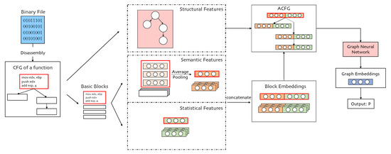
Figure 2.
The overall structure of SAViP. Semantic features are extracted by a pre-trained language model. Block embedding is the concatenation of semantic and statistical features. The structural feature is utilized in the graph neural network. Output P is the vulnerable probability of a function.
First, we use ida-python [38] (for IDA-PRO 7.0) to disassemble the binary program. Second, the assembly instructions and statistical characteristics of all target functions need to be extracted from the program. Among these, the selection of the target function will be explained in the experiment section. We use networkx [39] to retain the control information (structure information) of each function and the different attributes of each basic block (including assembly instructions and statistical vectors); the assembly instructions are collected for the subsequent semantic extraction step and will be used as the input of the language model after tokenization. Third, after obtaining the outputs (instruction embedding), we apply mean pooling to the outputs in the same basic block and form semantic block embeddings. Then, we merge these embeddings with the statistical vectors of the basic block to obtain the whole embedding of each basic block. All the block embeddings in a function and the link between the basic blocks together form an ACFG. The structural features will be input as an adjacency matrix in the following GNN. Although we say the input of the GNN is an ACFG graph, the real input is a feature matrix and an adjacency matrix. After passing the matrices through the GNN, they will finally go through a softmax layer to obtain the vulnerability prediction score of each function.
Next, we introduce the specific design details for each kind of feature separately.
3.2. Semantic Features
We apply the pre-training task of the RoBERTa [14] model to extract the semantics of assembly language. To train our language model on assembly language, we need to make our own dataset and perform appropriate pre-training to obtain a suitable model.
3.2.1. Tokenization
First, to capture the deep features from assembly statements, we need to tokenize the assembly instructions. We treat each instruction as a sentence; then, we standardize them with our rules and decompose them into basic tokens. For the definition of the basic token, we do not consider only the operand or only the operand type; instead, we divide the instructions more carefully, retaining richer information and keeping all of the opcodes and registers. For numbers, if the length of the hexadecimal form is longer than 6, we unify it as “”. If not, we regard it as meaningful and keep it. We then unify the variables as “”. For example, the instruction “mov [ebp+VAR_4] eax” is decomposed into “mov”, “[”, “ebp”, “+”, “”, “]”, and “eax” according to the rules.
After tokenizing the instructions, we obtain a set of standardized data that can be used for pre-training.
3.2.2. Pre-Training
After tokenization, we use the MLM task to pre-train our language model. The task replaces some of the tokens with “” in each epoch and trains the model to predict the original token. In this way, the model can learn the deep internal features of instructions. The MLM task needs specified inputs. According to the rules of the RoBERTa model, the first token of each input must be the special token “”, which marks the beginning of the input. After the training, the embedding of this special token can be used as the representation of the entire input. The last token entered is also a special token, “”, which corresponds to the start token and marks the end of the input. In addition, as shown in Figure 3, we also need segmentation and position embeddings and then mix the three tokens as the final input. Position embeddings are used to identify the position of each token, while segmentation embeddings can identify different sentences in the input. The mixed embeddings can enhance the model’s ability to represent tokens in different situations.
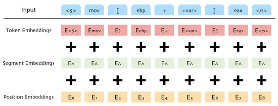
Figure 3.
Input embeddings of SAViP.
3.2.3. Dynamic Masking
While pre-training the model with data, we retain the MLM with dynamic masking. In BERT, the masking of the MLM task is static, and all masks are generated during the data processing stage. In all epochs, the masked token is fixed and will not be changed. In other words, the tokens that can be trained are limited. In contrast, dynamic masking delays the masking operation until the data are sent to the model, which can improve its expressive ability. A comparison between dynamic and static masking is shown in Figure 4. It is noteworthy that BERT replicates the sample 10 times, resulting in 10 different mask positions. To facilitate comparison and display, only one position is shown in the figure.
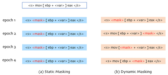
Figure 4.
Comparison between static masking and dynamic masking. Dynamic masking can mask more positions than static masking.
3.2.4. Outputs
After obtaining the pre-trained model, a series of layer values in the model can be obtained for each instruction. We regard the last hidden layer as the embedding. Among them, the first vector in the hidden layer corresponds to the “” token since it will be added at the front end before the input. Hence, this vector can represent the characteristics of the entire sentence. In addition, we consider the opcode to occupy a more important position than the operands in the assembly instructions. Therefore, we concatenate the embeddings of “” and the opcode as the instruction embedding, as shown in Figure 5. However, to build ACFGs, we need basic block embeddings. Therefore, we use mean pooling to process all the instruction embeddings in a basic block; that is, the embeddings of all instructions in a basic block are averaged to obtain the semantic embedding of each basic block.
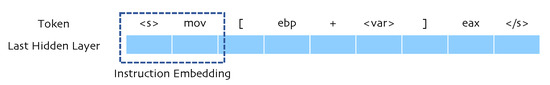
Figure 5.
Instruction embedding.
3.3. Statistical Features
Different from the complex semantic features which are hard for a computer to understand, statistical information can directly represent some characteristics of the assembly codes. As shown in Table 1, our statistical features mainly consist of three parts: instructions, operands, and special strings.

Table 1.
List of statistical features.
First, for the choice of instructions, V-Fuzz [12] arbitrarily selects 244-dimensional instruction-related features, resulting in a total feature count of 255 dimensions, which greatly increases the difficulty of training the neural networks. To reduce training overhead, improve efficiency, and avoid confusion caused by useless features, we should reduce the number of instructions considered. Inspired by Gemini [40], we count the four most common types of instructions: data transfer instructions, binary arithmetic instructions, logical instructions, and control transfer instructions. These instructions tend to influence memory and easily lead to vulnerabilities. Table 2 shows the details of the instruction list.
Table 2.
Instruction List.
There are eight common operands in total. Each type of operand has a different connotation, and we perform separate statistics on each of them. In addition, we pay attention to five specific strings, “malloc,” “calloc”, “free”, “memcpy” and “memset”, which are related to specific memory operations. The detection of these strings can help guide the improvement of the ability of the model to detect memory-related vulnerabilities in the evaluations.
In summary, we screen 43 instructions, 8 operand types, and 5 special strings, and obtain a 56-dimensional vector of statistical features, and, thus, each basic block can also be represented as a 56-dimensional vector containing statistical features. To verify the effectiveness of reducing the dimensions of statistical features, we conduct a comparative experiment in the experimental part of the paper. The experimental results demonstrate that our new statistical objects can retain most characteristics and reduce time costs.
3.4. Structural Features
For the graph, we use an improved structure2vec network. We train the network through a labeled dataset so that it can unearth the structural information of the assembly function. After obtaining the advanced node representation, we perform mean pooling on the block embeddings in a graph and use the result as the graph embedding. Then, we obtain the vulnerability probability for each function through a normalization layer and a softmax layer. In general, this neural network is similar to a two-class classification, but different from the latter, we need to output a value that is the probability that the function will eventually be predicted as a vulnerability.
3.4.1. Model Structure
Next, we will describe the composition of the neural network in detail. Figure 6 shows the overall flow of our improved GNN. F is the feature matrix, composed of all the basic block feature vectors in ACFG; A is the adjacency matrix of the ACFG plus a self-loop. The increase of the self-loop ensures that each basic block always maintains self-attention while collecting information from its neighbors. Assuming that the ACFG has p nodes and the dimension of the block embedding is , then F is a matrix, and A is a matrix. In this GNN, we establish a matrix of dimension to extract the information of each node, where e is the dimension of the final graph embedding vector. is initialized to a matrix of , that is, . We update the node information by continuously calculating a new as follows:
where is a matrix, and is a neural network connected by d-layer fully connected layers. In actual implementation, after each fully connected layer, a nonlinear layer needs to be connected to improve the expressive ability of the model. performs normalization and rectification (via a ReLU) on the result of the summation. Note that the operations here cannot be omitted, as they can effectively prevent gradient dispersion and improve the training effect. After T iterations, we obtain the latest graph feature matrix , the dimensions of which are still , and then we can obtain the embedding of the ACFG graph through transformation:
is a mean pooling layer, and the dimension of the embedding after pooling becomes . is an matrix. Therefore, the final dimension of the graph embedding is . Afterward, to obtain the security and vulnerability scores, we transform to obtain a two-dimensional vector Z =
where is a matrix. At this time, there is no constraint between the two values of Z. We next desire to obtain a meaningful output in the form :
In this equation, performs a nonlinear transformation on Z. Among this, a softmax layer and a normalization layer are used, and we can obtain the Q = , where p is the final output and represents the probability of vulnerabilities in the ACFG graph.

Figure 6.
Structure of the graph neural network. The input ACFG is divided into two matrices: a feature matrix and an improved adjacency matrix with a self-loop. The output is the vulnerability probability of the ACFG.
Figure 6.
Structure of the graph neural network. The input ACFG is divided into two matrices: a feature matrix and an improved adjacency matrix with a self-loop. The output is the vulnerability probability of the ACFG.

3.4.2. Model Training
To improve the ability to understand and distinguish secure and vulnerable functions, we need to set the labels for the training dataset in advance. The label l can take on a value of either 0 or 1, where 0 means the function is vulnerable, and 1 means it is secure. Given that our network structure and purpose are similar to those of the classification problem, we use the cross-entropy function to calculate the loss and update the model parameters with a stochastic gradient descent method.
4. Evaluation
4.1. Dataset
Almost all of the other works in vulnerability detection use the dataset processed by themselves and their source code is not being published. However, to better evaluate our work, we still try to reproduce the whole project of V-Fuzz and make a comparison with it. Hence, we use the Juliet Test Suite (v1.3) [18] for our model training and testing, which has been widely utilized in previous vulnerability-related studies [5,12,41]. This dataset was released by the National Institute of Standards and Technology (NIST) in 2017 and involves 118 different common weakness enumeration (CWE) entities and 64,099 cases. All testcases are written in C/C++, and each function is labeled with “good” or “bad”, where “good” mean “secure” and “bad” means “vulnerable”. Among the 118 CWE entities in the Juliet Test Suite, we select 12 memory-related entities to better compare our model with V-Fuzz, which uses the same CWEs. The Juliet Test Suite differentiates functions as “source” and “sink”. Whereas source functions generate the data, sink functions utilize the data and are more closely related to program crashes. Thus, we select the sink functions and construct our dataset. The specific types of CWE and the number of labeled functions are recorded in Table 3. To train the model for each type of vulnerability equally, we attempt to include the same number of positive and negative cases in each CWE. If the total number is less than the target number, we sample from the overall legacy data to complete the dataset. Table 4 shows the data volume of each dataset. We extract a total of 22,000 positive cases and 22,000 negative cases; the training set contains 18,000 of each, and the test and development sets contain 2000 of each.
Table 3.
Types of CWE.
Table 4.
Dataset statistics.
4.2. Environment
We implement the model on PyTorch, which is widely used in deep learning tasks. For the hardware configuration, we train the model on a server with an Intel Xeon CPU E5-2680v3@2.50 GHz, one GeForce GTX 2080Ti GPU, and 94 GB memory.
4.3. Evaluation Metrics
Since one of the most important proposed motivations of our model is to guide dynamic analysis, we desire to use a higher score to reflect higher accuracy. In this way, we could be confident when choosing the direction of dynamic analysis (e.g., seed mutation in fuzzing) based on the score. Therefore, we use two metrics, accuracy, and recall, to evaluate the model, which is defined in V-Fuzz. In this way, we can test the effectiveness of our work and also make a better comparison with V-Fuzz.
First, we make explanations for these two metrics as follows. Suppose there are L cases, in which the number of “vulnerable” cases is A and the number of “secure” cases is L-A. Passing L cases into the model generates L scores (vulnerable probability). We sort the scores in reverse order and take the first N scores. If the number of cases with the true label of “vulnerable” is n among these N cases, we say that the K-N (e.g., K-100 or K-200) accuracy is . If we set N to A, the K-A accuracy is . Since A is the number of “vulnerable” cases out of all cases, K-A is also defined as the recall rate.
4.4. Model Performance
According to the above metrics, the performance of our model on the validation set is shown in Figure 7. Figure 7a shows the corresponding accuracies when we set different values of K. The accuracy rapidly improves between epochs 0 and 20 and is essentially maximum at 40 epochs, fluctuating around the maximum thereafter. Obviously, the smaller the K value is, the higher the accuracy. This shows that our scores are meaningful: the higher the score is, the higher the confidence in the prediction and the greater the probability of vulnerabilities. In addition, the curves for K = 100∼1000 are all above 90% in the end, while those for K = 100∼600 reach above 95%. Since there is no open source of V-Fuzz, we implement the prediction model of V-Fuzz (according to the parameters in the paper) and conduct experiments on the same dataset used for SAViP. Figure 7b shows the Top-K accuracies for V-Fuzz. The accuracies for K = 100∼600 surpass 82%, indicating that SAViP is 13% better than V-Fuzz. Figure 7c shows the comparison of the recall of the two models; V-Fuzz reaches 0.6775, which is slightly better than its performance in the original paper; this is because our standards for dataset labeling are not totally same with it. Figure 7c clearly shows that the recall of our model and V-Fuzz increase in similar manners, and both reach the highest value around epoch 40. Our recall increases from 50% to 78%, which is 11% higher than V-Fuzz. These comparisons indicate that our model makes improvements over the state-of-the-art V-Fuzz.
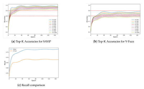
Figure 7.
Performance comparison of SAViP and V-Fuzz. For both the Top-K accuracies and recall, SAViP performs better than V-Fuzz.
In addition, we distinguish the performance of each CWE. To assess the confidence for the highest-scoring data, we take the K-10 accuracy for each CWE. Figure 8 shows the K-10 accuracy and recall of SAViP and the recall of V-Fuzz for each CWE. The two dashed lines in the figure are the 95% accuracy baseline and the 78% recall baseline. We can see that, for the K-10 accuracy, only CWE134 and CWE401 reach 95% and 90% accuracy, respectively, while the rest reach 100%. This shows that our model exhibits high confidence in the vulnerability scores, which means that a high-scoring function has a high probability of possessing vulnerability. In terms of the recall rate, SAViP performs better than V-Fuzz for all of the CWEs. More specifically, for SAViP, 6 CWEs possess a recall higher than the baseline (i.e., the recall overall), while the recall of the other 6 CWEs is lower. This shows that the performance of our model is balanced; that is, the overall performance improvement over V-Fuzz does not originate from the extreme performances of individual CWEs.
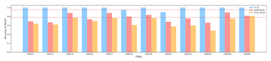
Figure 8.
Model performance for different CWEs. The Top 10 accuracy of SAViP reaches 100% except for CWE134 and CWE401. For recall, SAViP outperforms V-Fuzz for all CWEs.
Summary: SAViP outperforms the state-of-the-art approach V-Fuzz in vulnerability prediction with a large margin. It can automatically predict vulnerabilities without prior knowledge predefined by security experts, which reduces the burden on researchers.
4.5. Ablation Study
Although we have demonstrated the effectiveness of our model, it is also important to determine which feature contributes the most to the result. To this end, we conduct an ablation study to analyze the role of each kind of feature. We evaluate the results from two perspectives: recall and the average training time per epoch. Figure 9 shows the training curves under different settings, and Table 5 provides a more direct representation of their differences with various evaluation metrics. The column called GAP shows the impact of each missing feature on the recall rate of model testing, using percentages to increase the contrast.
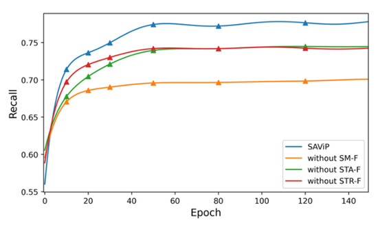
Figure 9.
Results of the ablation study. The graph shows that the most significant contribution to our model was made by semantic features.
Table 5.
Ablation Study.
From the results, removing semantic features (SM-F) reduces the recall by 8.8%, which shows that this part of the model improves recall the most. However, it is also the most time-consuming part, as the training time difference for an epoch reaches 6.18 s. The addition of statistical features (STA-F) and structural features (STR-F) has similar effects on performance, with recall differences of less than 5%. However, structure feature extraction involves the GNN, which leads to more time consumption (5 s) than statistical feature extraction.
As mentioned above, the ablation study shows that semantic features contribute the most to our vulnerability prediction model. This proves that semantic learning can penetrate deeply into basic blocks and can extract more complex details than statistical information.
4.6. Parameter Analysis
In the process of exploring the best parameter settings, we regard recall as the most important evaluation metric. For parameters with similar recall values, the training time is used as the second evaluation index. We average the total time for 150 epochs to obtain the time for one epoch.
4.6.1. Semantic Features
We apply the pre-training task from RoBERTa to extract assembly semantics and obtain instruction embeddings and then the semantic embedding of basic blocks. Instruction embeddings are similar to sentence embeddings in natural language; they are commonly obtained by selecting vector corresponding to the first special token “” as the sentence embedding. Considering the importance of opcodes in assembly language, we concatenate “” with the vector of opcodes. To demonstrate the correctness of this procedure, we distinguish several different RoBERTa settings for comparison. Table 6 and Figure 10a show the specific setting differences and the final experimental results. Among them, we also test the effects of different embedding dimensions (32, 64, 128, and 128) and compare the results when the subsequent designs are exactly the same. The result shows that, when 64 dimensions are used as the word embedding size, the result of using both “” and opcode is better than using either alone. When the two are used alone, the recall and time consumption are very similar, indicating that the implicit features in these two are similar but complementary. This demonstrates the superiority of our design. In the testing of the embedding dimension, we can see that the higher the dimension, the higher the recall is, but the longer the time consumed. To balance the recall and time costs, we choose 64 as the final word embedding size.
Table 6.
Language model experiments.
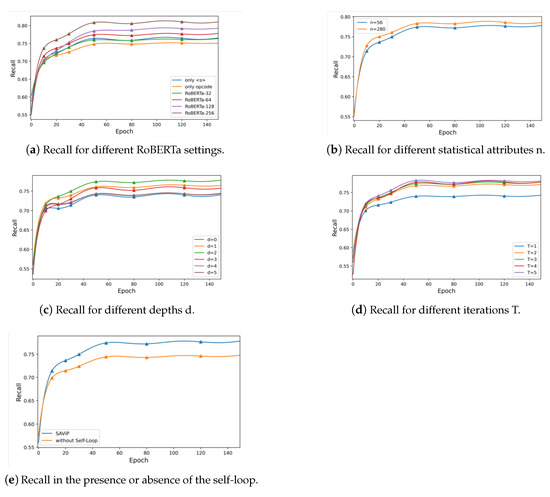
Figure 10.
Results for different training settings.
4.6.2. Statistical Features
In the model design section, we introduce the details of the 56-dimensional feature vectors. We compare this design with V-Fuzz, which uses all of the instructions. According to the Software Developer’s Manual [15] released by Intel in March 2020, we set a total of 280-dimensional vectors for the latter. Table 7 (Statistical Size) and Figure 10b show the recall and the corresponding training time comparison generated by the two cases. We find that, although the recall obtained for the latter is slightly higher, the time costs are greatly increased. We consider spending 50% more time for less than 1% improvement to be illogical, so we use the 56-dimensional solution.
Table 7.
Parameter experiments.
4.6.3. Structural Features
- DepthTable 7(Depth) and Figure 10c show the influence of different neural network depths d in the model. By setting the number of fully connected layers d (d = 0∼5), we observe that the recall reaches its maximum value when d is 2. We believe that the reason is that an excessively deep network structure will result in feature dispersion, leading to worse results. Therefore, we choose 2 as the final depth of the network in the GNN.
- Iteration In the GNN, we need to perform certain iterations to optimize the parameters. We set T to 1, 2, 3, 4, and 5 to observe the impact of iterations on the network. Table 7 (Iteration) and Figure 10d show the differences in the recall for different situations. The recall obtained in cases where are very similar, but the larger T is, the greater the time cost. We infer that the scale is not sufficiently large to require deep iterations; for our functions, three hops are sufficient for the basic blocks to collect the information of their neighbors. Therefore, we set T to 3 as the number of iterations of the GNN.
- Self-Loop To ensure the block embeddings always focus on themselves while collecting network information, we add a self-loop to the ACFG before the GNN starts. Table 7 (Self-Loop) and Figure 10e show the effect of this step on the results. The experimental results show that, after adding the self-loop, the recall is increased by 3.7%. This shows that the addition of a self-loop can improve the ability of the GNN to extract structural features well.
In summary, after multiple experimental verifications, we set the word embedding vector size to 64 and merge the embeddings of “” and the opcode as the instruction embedding. We design a vector of 56 dimensions to represent statistical features. In the GNN, we set the network depth to 2 and the number of iterations to 3. In addition, in terms of implementation details, we set the batch size to 32, the initial learning rate to 0.01, and attenuation is performed every 50 epochs.
5. Conclusions
In this paper, we propose a vulnerability prediction model that extracts three kinds of features—the semantic, the statistical, and the structural features—to represent vulnerability characteristics. For the semantic features, we apply the MLM pre-training task of the RoBERTa model to assembly language to train our language model and then generate instruction embeddings through it. To combine more comprehensive semantics, we design a 56-dimensional statistical feature and a structural feature to integrate instruction counts and CFG structures. We implement this prediction model as a prototype named SAViP. Experiments show that SAViP outperforms the state-of-the-art method V-Fuzz in vulnerability prediction by 10% and 13% in recall and accuracy, respectively. SAViP automatically predicts vulnerabilities without prior vulnerability patterns predefined by security experts, which provides an effective method to detect vulnerabilities and reduces the burden on researchers.
Author Contributions
Methodology, X.Z.; Software, B.D. and X.W.; Formal analysis, P.W. All authors have read and agreed to the published version of the manuscript.
Funding
This research was funded by the National University of Defense Technology Research Project (ZK20-17, ZK20-09), the National Natural Science Foundation China (62272472, 61902405), the HUNAN Province Natural Science Foundation (2021JJ40692), the National Key Research and Development Program of China under Grant No. 2021YFB0300101, and the National High-level Personnel for Defense Technology Program (2017-JCJQ-ZQ-013).
Data Availability Statement
Not applicable.
Conflicts of Interest
The authors declare no conflict of interest.
References
- SonarQube. Available online: https://www.sonarqube.org/ (accessed on 7 January 2022).
- DeepScan. Available online: https://deepscan.io/ (accessed on 7 January 2022).
- Reshift Security. Available online: https://www.reshiftsecurity.com/ (accessed on 7 January 2022).
- Wang, S.; Liu, T.; Tan, L. Automatically Learning Semantic Features for Defect Prediction. In Proceedings of the 2016 IEEE/ACM 38th International Conference on Software Engineering, Austin, TX, USA, 14–22 May 2016; pp. 297–308. [Google Scholar]
- Li, Z.; Zou, D.; Xu, S.; Ou, X.; Jin, H.; Wang, S.; Deng, Z.; Zhong, Y. VulDeePecker: A deep learning-based system for vulnerability detection. In Proceedings of the 25th Network and Distributed System Security Symposium, San Diego, CA, USA, 18–21 February 2018; pp. 1–15. [Google Scholar]
- Wang, S.; Liu, T.; Nam, J.; Tan, L. Deep Semantic Feature Learning for Software Defect Prediction. IEEE Trans. Softw. Eng. 2020, 46, 1267–1293. [Google Scholar] [CrossRef]
- Luo, Z.; Wang, P.; Wang, B.; Tang, Y.; Xie, W.; Zhou, X.; Liu, D.; Lu, K. VulHawk: Cross-architecture Vulnerability Detection with Entropy-based Binary Code Search. In Proceedings of the 2023 Network and Distributed System Security Symposium, San Diego, CA, USA, February 2023. [Google Scholar]
- Zheng, J.; Pang, J.; Zhang, X.; Zhou, X.; Li, M.; Wang, J. Recurrent Neural Network Based Binary Code Vulnerability Detection. In Proceedings of the 2019 2nd International Conference on Algorithms, Computing and Artificial Intelligence, Hong Kong, China, 20–22 December 2019; pp. 160–165. [Google Scholar]
- Han, W.; Pang, J.; Zhou, X.; Zhu, D. Binary vulnerability mining technology based on neural network feature fusion. In Proceedings of the 2022 5th International Conference on Advanced Electronic Materials, Computers and Software Engineering (AEMCSE), Wuhan, China, 22–24 April 2022; pp. 257–261. [Google Scholar]
- Duan, B.; Zhou, X.; Wu, X. Improve vulnerability prediction performance using self-attention mechanism and convolutional neural network. In Proceedings of the International Conference on Neural Networks, Information, and Communication Engineering (NNICE), Guangzhou, China, June 2022. [Google Scholar]
- Tian, J.; Xing, W.; Li, Z. BVDetector: A program slice-based binary code vulnerability intelligent detection system. Inf. Softw. Technol. 2020, 123, 106289. [Google Scholar] [CrossRef]
- Li, Y.; Ji, S.; Lyu, C.; Chen, Y.; Chen, J.; Gu, Q. V-Fuzz: Vulnerability-Oriented Evolutionary Fuzzing. arXiv 2019, arXiv:1901.01142. [Google Scholar]
- Mikolov, T.; Chen, K.; Corrado, G.; Dean, J. Efficient estimation of word representations in vector space. arXiv 2013, arXiv:1301.3781. [Google Scholar]
- Liu, Y.; Ott, M.; Goyal, N.; Du, J.; Joshi, M.; Chen, D. Roberta: A robustly optimized bert pretraining approach. arXiv 2019, arXiv:1907.11692. [Google Scholar]
- Intel. Available online: https://software.intel.com/en-us/articles/intel-sdm (accessed on 7 January 2022).
- Feng, Q.; Zhou, R.; Xu, C.; Cheng, Y.; Testa, B.; Yin, H. Scalable graph-based bug search for firmware images. In Proceedings of the 2016 ACM SIGSAC Conference on Computer and Communications Security, New York, NY, USA, 24–28 October 2016; pp. 480–491. [Google Scholar]
- Dai, D.H.; Dai, B.; Song, L. Discriminative embeddings of latent variable models for structured data. In Proceedings of the International Conference on Machine Learning, New York, NY, USA, 19–24 June 2016; pp. 2702–2711. [Google Scholar]
- Software Assurance Reference Dataset. Available online: https://samate.nist.gov/SRD/testsuite.php (accessed on 7 January 2022).
- Zou, D.; Wang, S.; Xu, S.; Li, Z.; Jin, H. μVulDeePecker: A Deep Learning-Based System for Multiclass Vulnerability Detection. IEEE Trans. Dependable Secur. Comput. 2021, 18, 2224–2236. [Google Scholar] [CrossRef]
- LLVM Compiler Infrastructure. Available online: https://llvm.org/docs/LangRef.html (accessed on 7 January 2022).
- Zaremba, W.; Sutskever, I.; Vinyals, O. Recurrent neural network regularization. arXiv 2014, arXiv:1409.2329. [Google Scholar]
- Cho, K.; Van Merriënboer, B.; Gulcehre, C.; Bahdanau, D.; Bougares, F.; Schwenk, H. Learning phrase representations using RNN encoder-decoder for statistical machine translation. arXiv 2014, arXiv:1406.1078. [Google Scholar]
- Rawat, S.; Jain, V.; Kumar, A.; Cojocar, L.; Giuffrida, C.; Bos, H. VUzzer: Application-aware Evolutionary Fuzzing. In Proceedings of the 25th Network and Distributed System Security Symposium, San Diego, CA, USA, 26 February–1 March 2017; Volume 17, pp. 1–14. [Google Scholar]
- Zhang, G.; Zhou, X.; Luo, Y.; Wu, X.; Min, E. Ptfuzz: Guided fuzzing with processor trace feedback. IEEE Access 2018, 6, 37302–37313. [Google Scholar] [CrossRef]
- Song, C.; Zhou, X.; Yin, Q.; He, X.; Zhang, H.; Lu, K. P-fuzz: A parallel grey-box fuzzing framework. Appl. Sci. 2019, 9, 5100. [Google Scholar] [CrossRef]
- Xu, K.; Hu, W.; Leskovec, J.; Jegelka, S. How powerful are graph neural networks? arXiv 2018, arXiv:1810.00826. [Google Scholar]
- Devlin, J.; Chang, M.W.; Lee, K.; Toutanova, K. Bert: Pre-training of deep bidirectional transformers for language understanding. arXiv 2018, arXiv:1810.04805. [Google Scholar]
- Vaswani, A.; Shazeer, N.; Parmar, N.; Uszkoreit, J.; Jones, L.; Gomez, A.N. Attention is all you need. In Proceedings of the Advances in Neural Information Processing Systems, Long Beach, CA, USA, 4 December 2017; pp. 5998–6008. [Google Scholar]
- Kumar, S.; Chaudhary, S.; Kumar, S.; Yadav, R.K. Node Classification in Complex Networks using Network Embedding Techniques. In Proceedings of the 2020 5th International Conference on Communication and Electronics Systems, Coimbatore, India, 10–12 June 2020; pp. 369–374. [Google Scholar]
- Mithe, S.; Potika, K. A unified framework on node classification using graph convolutional networks. In Proceedings of the 2020 Second International Conference on Transdisciplinary AI, Irvine, CA, USA, 21–23 September 2020; pp. 67–74. [Google Scholar]
- Deylami, H.A.; Asadpour, M. Link prediction in social networks using hierarchical community detection. In Proceedings of the 2015 7th Conference on Information and Knowledge Technology, Urmia, Iran, 26–28 May 2015; pp. 1–5. [Google Scholar]
- Abbasi, F.; Talat, R.; Muzammal, M. An Ensemble Framework for Link Prediction in Signed Graph. In Proceedings of the 2019 22nd International Multitopic Conference, Islamabad, Pakistan, 29–30 November 2019; pp. 1–6. [Google Scholar]
- Ting, Y.; Yan, C.; Xiang-wei, M. Personalized Recommendation System Based on Web Log Mining and Weighted Bipartite Graph. In Proceedings of the 2013 International Conference on Computational and Information Sciences, Shiyang, China, 21–23 June 2013; pp. 587–590. [Google Scholar]
- Suzuki, T.; Oyama, S.; Kurihara, M. A Framework for Recommendation Algorithms Using Knowledge Graph and Random Walk Methods. In Proceedings of the 2020 IEEE International Conference on Big Data, Atlanta, GA, USA, 10–13 December 2020; pp. 3085–3087. [Google Scholar]
- Perozzi, B.; Al-Rfou, R.; Skiena, S. Deepwalk: Online learning of social representations. In Proceedings of the 20th ACM SIGKDD International Conference on Knowledge Discovery and Data Mining, New York, NY, USA, 24–27 August 2014. [Google Scholar]
- Grover, A.; Leskovec, J. node2vec: Scalable feature learning for networks. In Proceedings of the 22nd ACM SIGKDD International Conference on Knowledge Discovery and Data Mining, San Francisco, CA, USA, 13–17 August 2016. [Google Scholar]
- Cao, S.; Lu, W.; Xu, Q. Grarep: Learning graph representations with global structural information. In Proceedings of the 24th ACM International on Conference on Information and Knowledge Management, Melbourne, Australia, 18–23 October 2015. [Google Scholar]
- Hex-Rays. Available online: https://www.hex-rays.com/products/ida/ (accessed on 7 January 2022).
- Networkx. Available online: https://networkx.org/ (accessed on 7 January 2022).
- Xu, X.; Liu, C.; Feng, Q.; Yin, H.; Song, L.; Song, D. Neural network-based graph embedding for cross-platform binary code similarity detection. In Proceedings of the 2017 ACM SIGSAC Conference on Computer and Communications Security, Dallas, TX, USA, 30 October–3 November 2017; pp. 363–376. [Google Scholar]
- Han, W.; Joe, B.; Lee, B.; Song, C.; Shin, I. Enhancing memory error detection for large-scale applications and fuzz testing. In Proceedings of the 25th Network and Distributed System Security Symposium, San Diego, CA, USA, 18–21 February 2018; pp. 1–47. [Google Scholar]


Disclaimer/Publisher’s Note: The statements, opinions and data contained in all publications are solely those of the individual author(s) and contributor(s) and not of MDPI and/or the editor(s). MDPI and/or the editor(s) disclaim responsibility for any injury to people or property resulting from any ideas, methods, instructions or products referred to in the content. |
© 2023 by the authors. Licensee MDPI, Basel, Switzerland. This article is an open access article distributed under the terms and conditions of the Creative Commons Attribution (CC BY) license (https://creativecommons.org/licenses/by/4.0/).