
Research on the Applicability of Transformer Model in Remote-Sensing Image Segmentation

Abstract
:1. Introduction
2. Methods
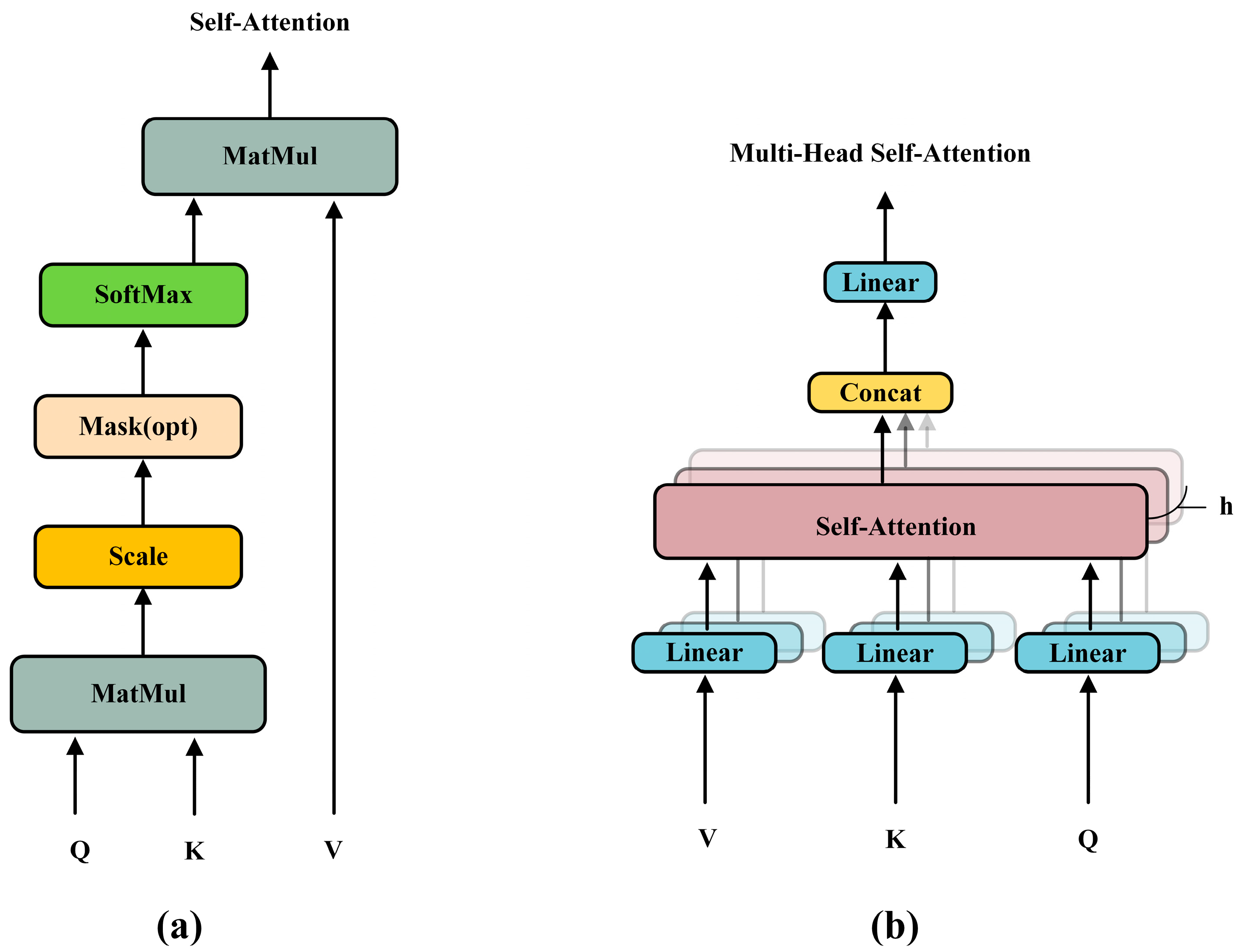
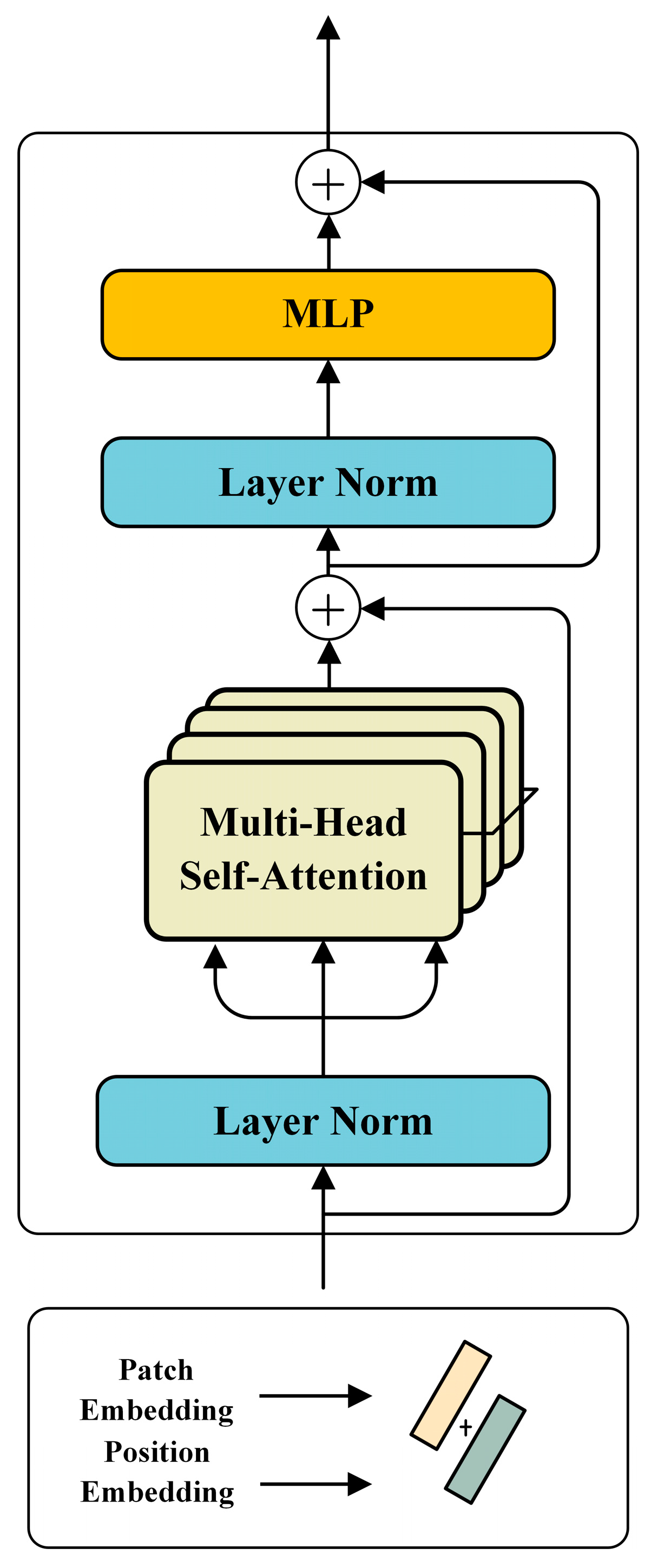
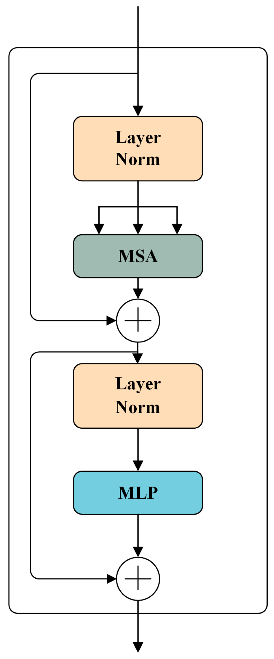
2.1. Transformer Model
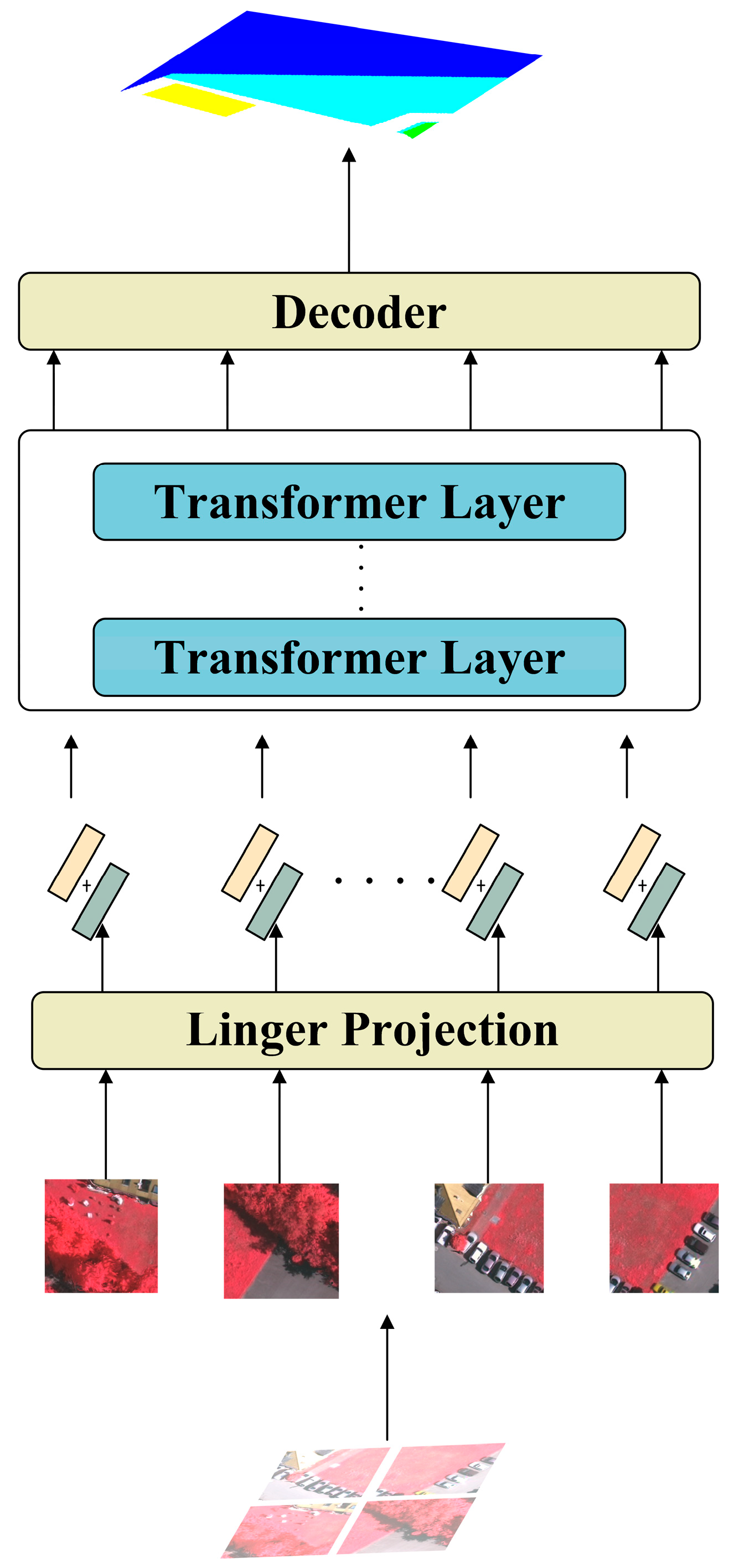
2.2. SETRnet (Segmentation Transformer)
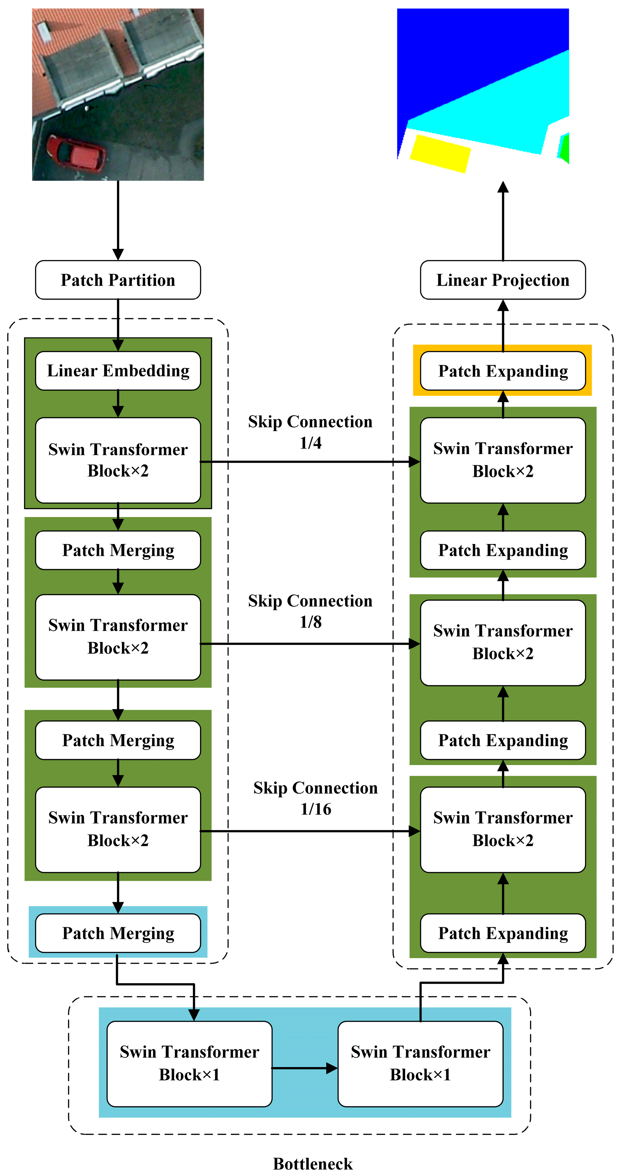
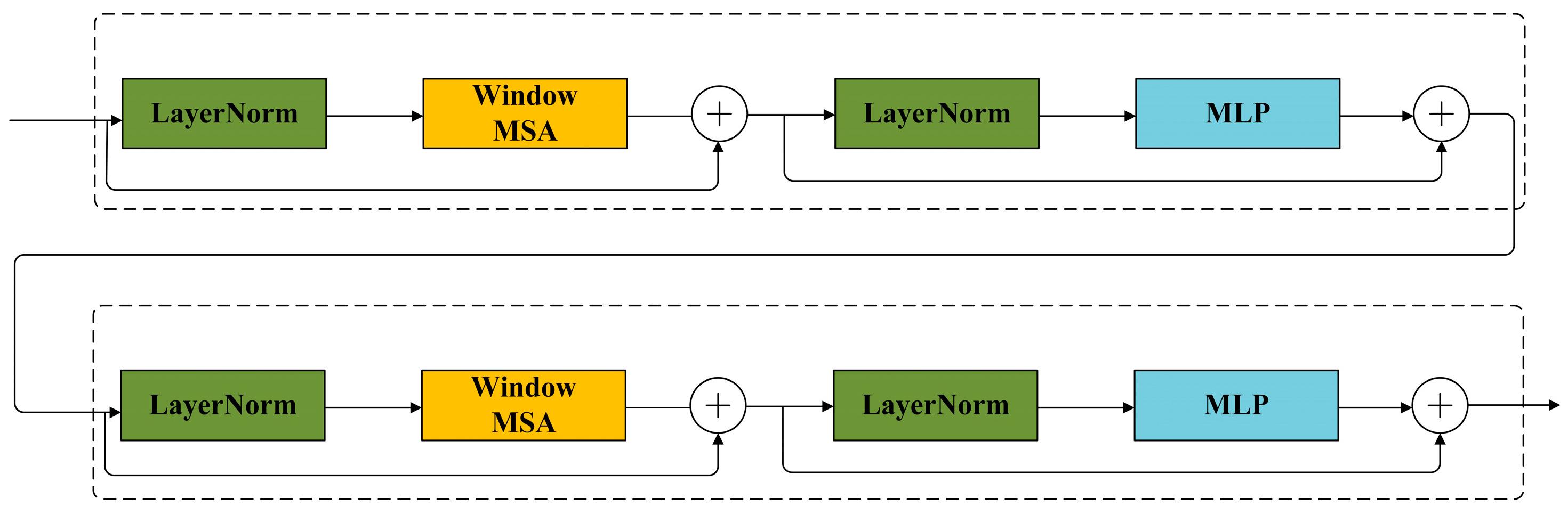
2.3. SwinUnet
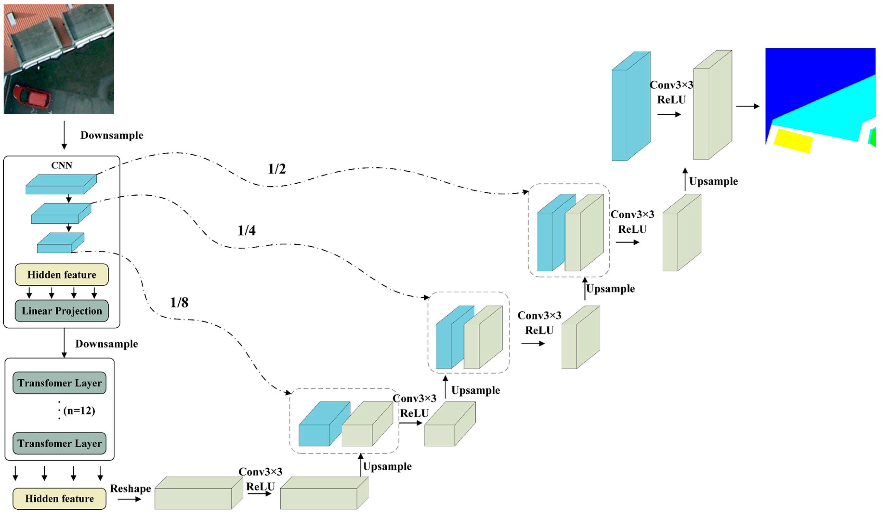
2.4. TransUnet
2.5. Accuracy Comparison of Models
2.6. Training Time Comparison of Models
3. Experiment and Results
3.1. Experimental Setup
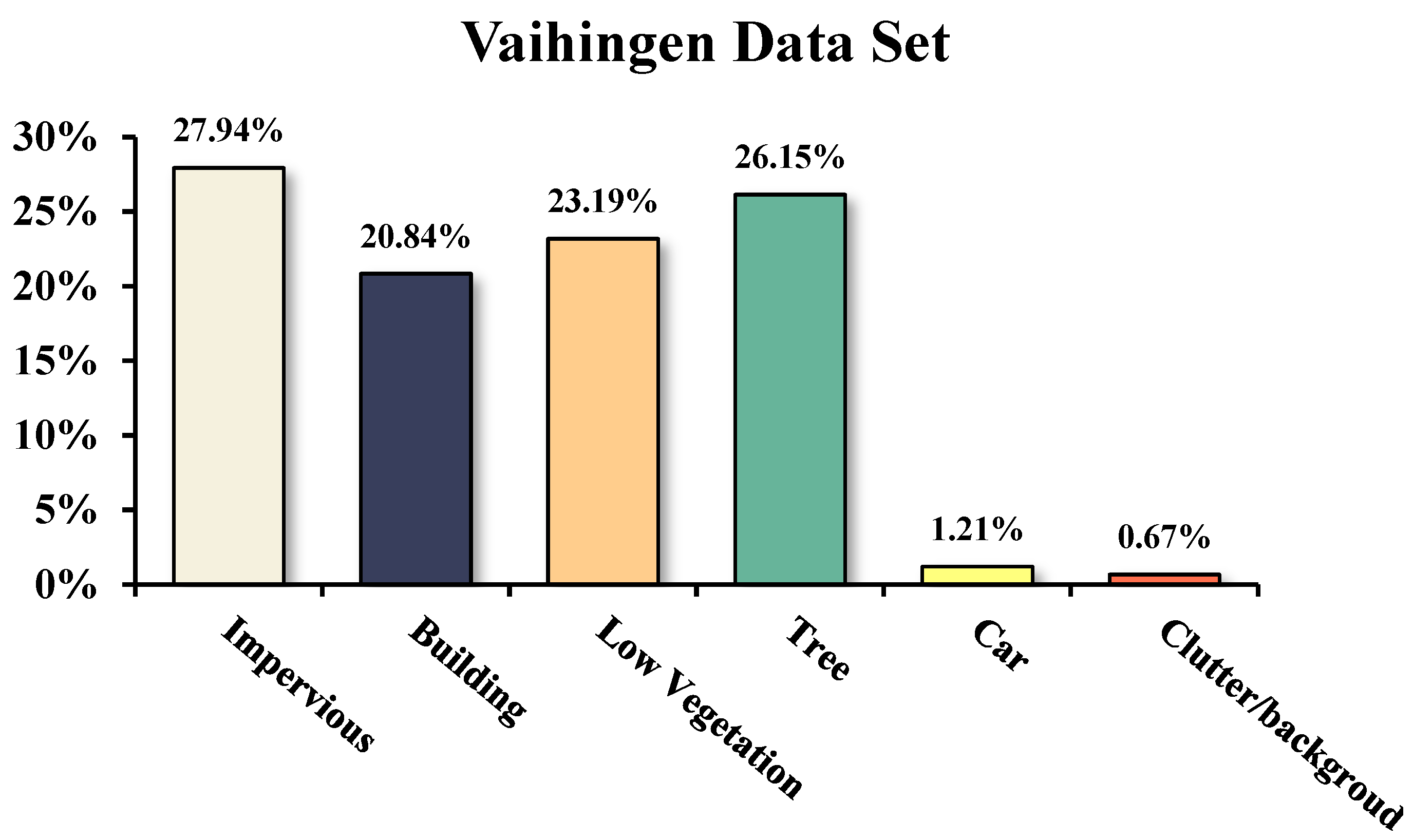
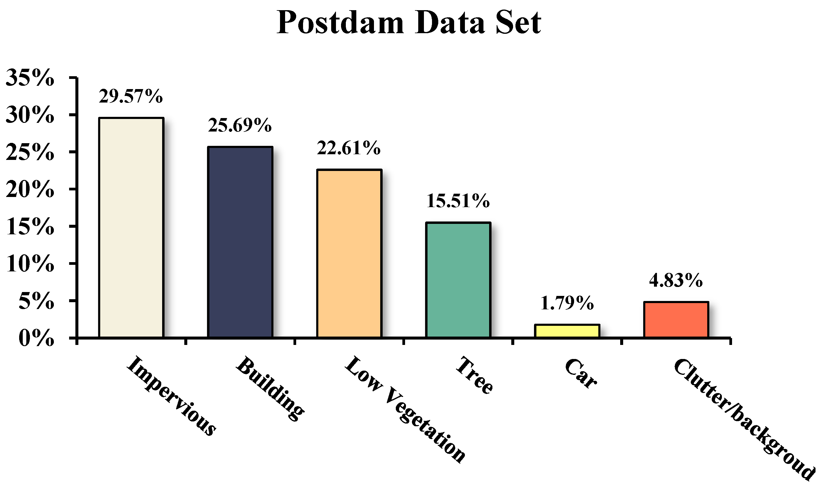
3.1.1. Data Set
3.1.2. Metrics
3.2. Result
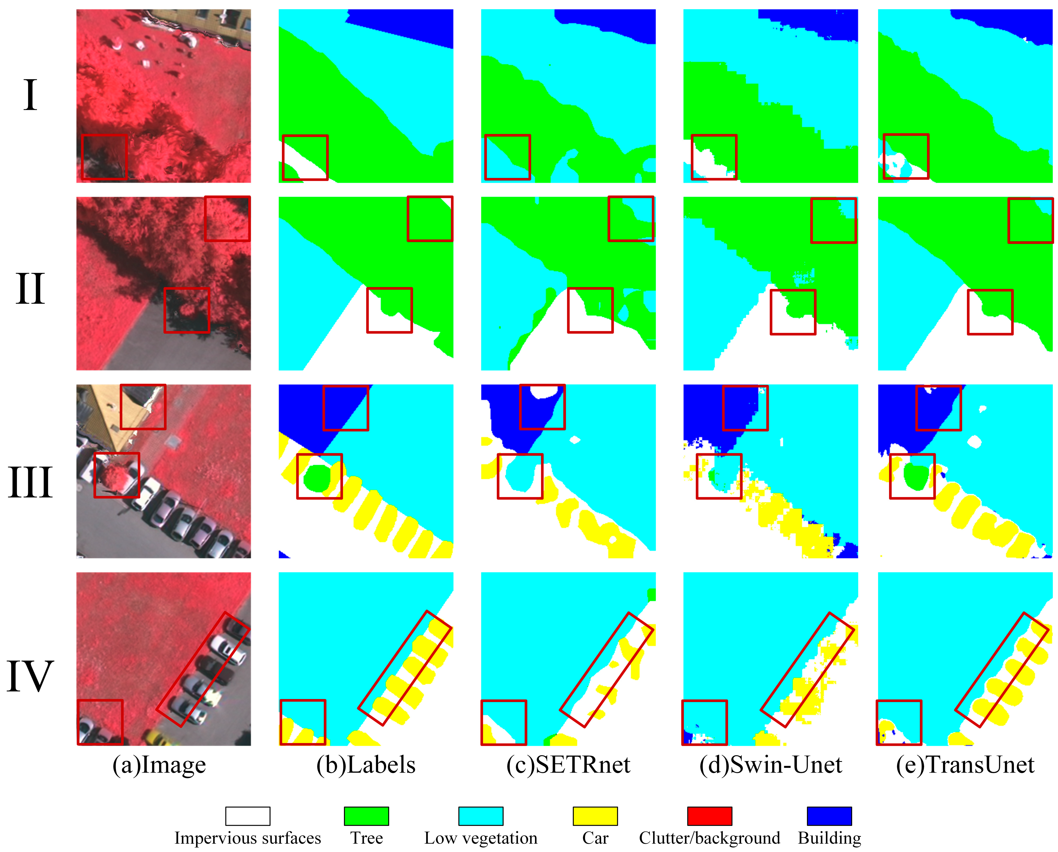
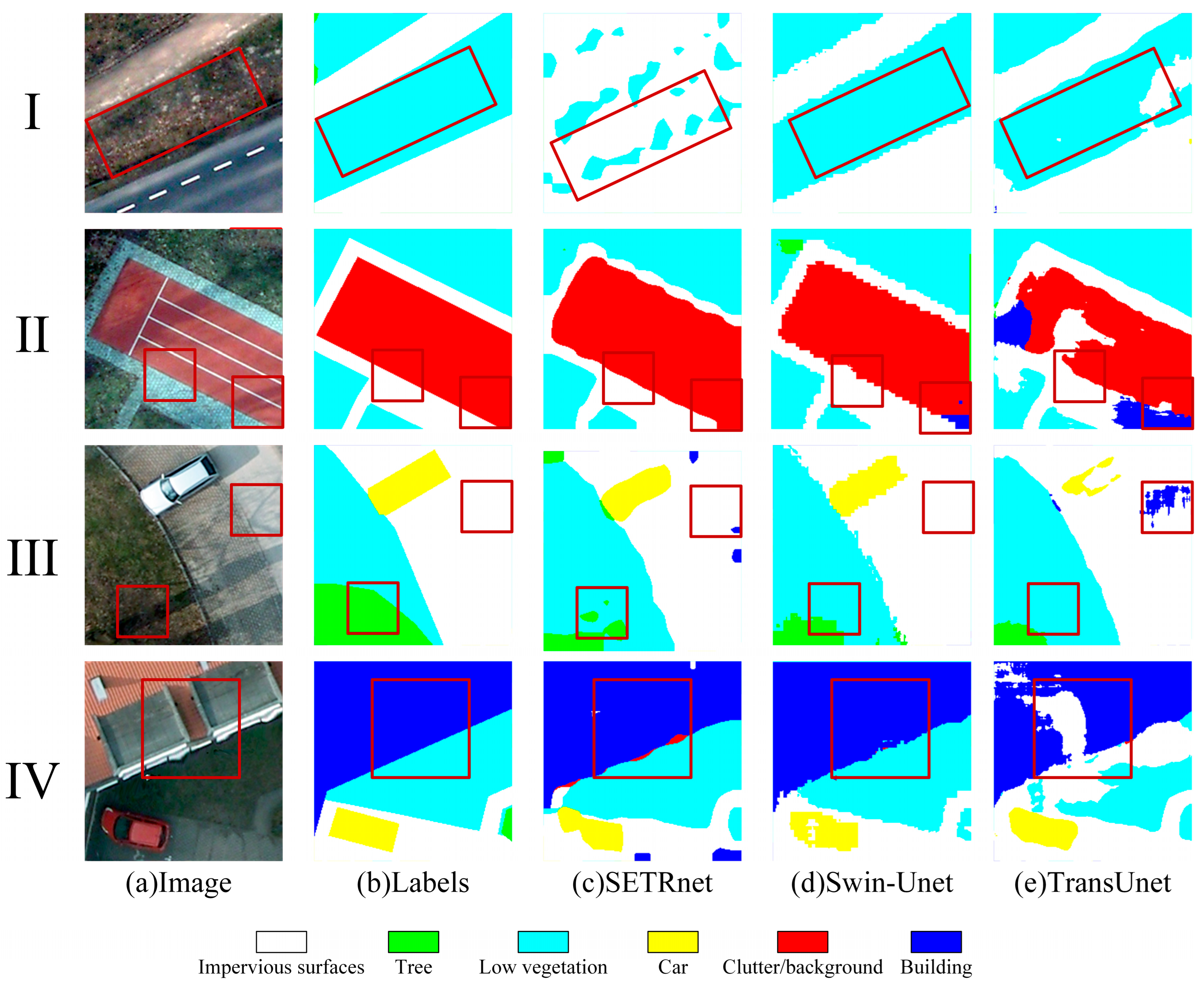
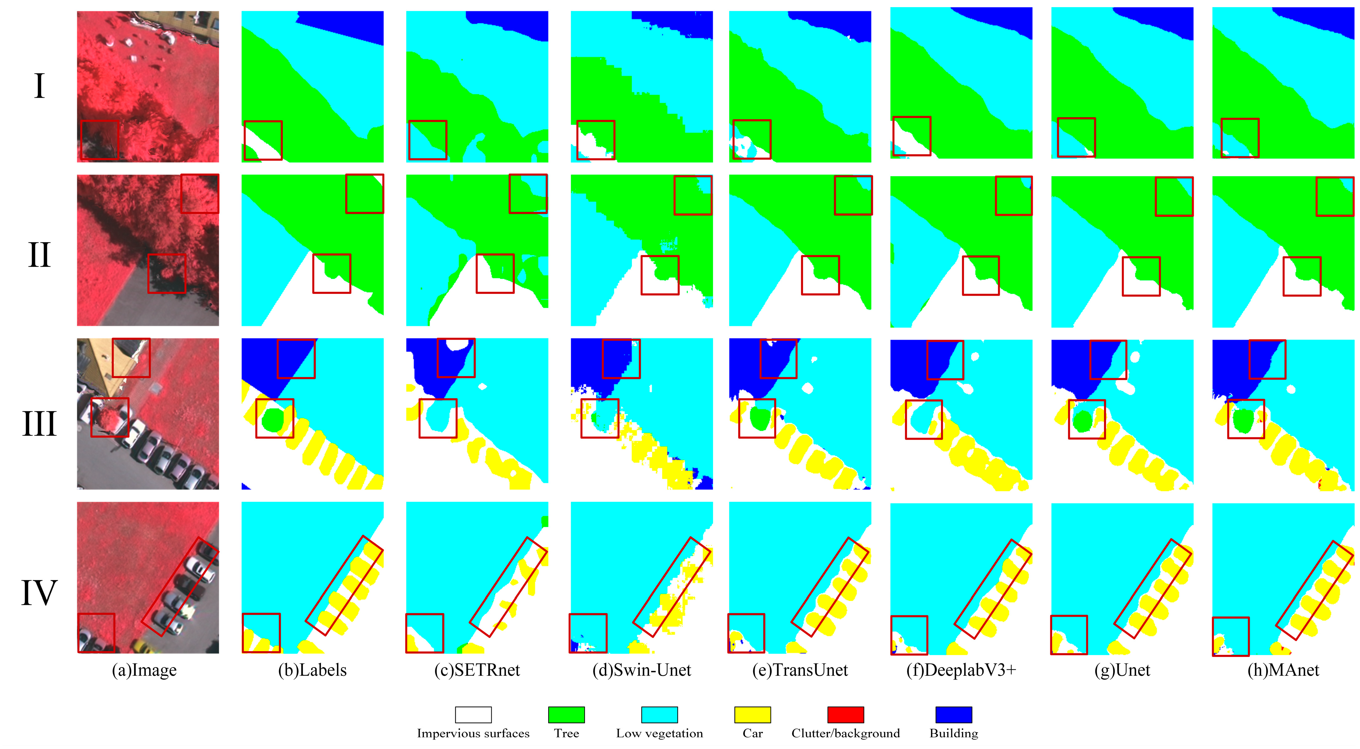
3.2.1. Metrics Visual Analysis of Classification Results
3.2.2. Training Time Comparison

| Method | SETRnet | SwinUnet | TransUnet |
|---|---|---|---|
| Time(s) | 4401.1 | 2929.7 | 6119.4 |
| Average time(s) | 110.03 | 73.24 | 152.99 |
| Method | SETRnet | SwinUnet | TransUnet |
|---|---|---|---|
| Time(s) | 38,877.1 | 26,405.7 | 27,399.3 |
| Average time(s) | 971.93 | 660.14 | 684.98 |
3.2.3. Accuracy Comparison of Results
3.2.4. Kappa Coefficient Effect Size Test
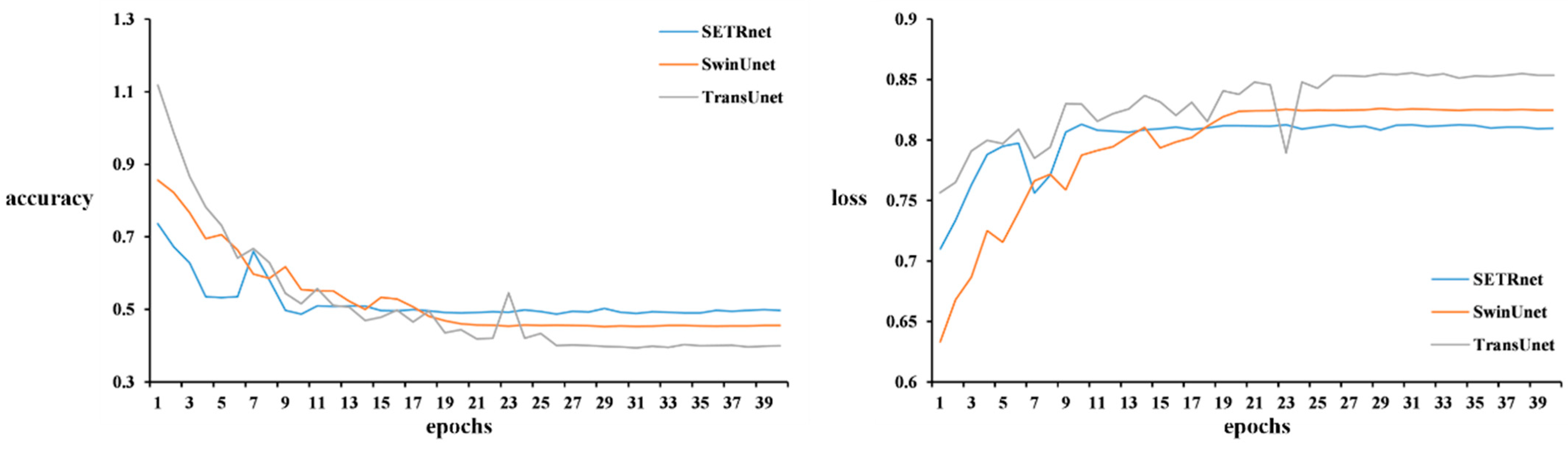
3.2.5. Training Process of Different Transformers
3.2.6. Comparison of CNNs
4. Discussion
5. Conclusions
Author Contributions
Funding
Institutional Review Board Statement
Informed Consent Statement
Data Availability Statement
Conflicts of Interest
References
- Srivastava, A.; Jha, D.; Chanda, S.; Pal, U.; Johansen, H.D.; Johansen, D.; Riegler, M.A.; Ali, S.; Halvorsen, P. MSRF-Net: A Multi-Scale Residual Fusion Network for Biomedical Image Segmentation. IEEE J. Biomed. Health Inform. 2022, 26, 2252–2263. [Google Scholar] [CrossRef]
- Beyaz, A.; Martínez Gila, D.M.; Gómez Ortega, J.; Gámez García, J. Olive Fly Sting Detection Based on Computer Vision. Postharvest Biol. Technol. 2019, 150, 129–136. [Google Scholar] [CrossRef]
- Beyaz, A.; Gerdan, D. Meta-Learning Based Prediction of Different Corn Cultivars from Colour Feature Extraction with Image Processing Technique. Tarım Bilim. Derg. 2021, 27, 32–41. [Google Scholar] [CrossRef]
- Yuan, J.; Wang, D.; Li, R. Remote Sensing Image Segmentation by Combining Spectral and Texture Features. IEEE Trans. Geosci. Remote Sens. 2014, 52, 16–24. [Google Scholar] [CrossRef]
- Kotaridis, I.; Lazaridou, M. Remote Sensing Image Segmentation Advances: A Meta-Analysis. ISPRS J. Photogramm. Remote Sens. 2021, 173, 309–322. [Google Scholar] [CrossRef]
- Ibrahim, A.; El-kenawy, E.-S.M. Image Segmentation Methods Based on Superpixel Techniques: A Survey. J. Comput. Sci. Inf. Syst. 2020, 15, 1–11. [Google Scholar]
- Xiong, D.; He, C.; Liu, X.; Liao, M. An End-To-End Bayesian Segmentation Network Based on a Generative Adversarial Network for Remote Sensing Images. Remote Sens. 2020, 12, 216. [Google Scholar] [CrossRef]
- Zheng, K.; Wang, H.; Qin, F.; Han, Z. A Land Use Classification Model Based on Conditional Random Fields and Attention Mechanism Convolutional Networks. Remote Sens. 2022, 14, 2688. [Google Scholar] [CrossRef]
- Misbah, K.; Laamrani, A.; Khechba, K.; Dhiba, D.; Chehbouni, A. Multi-Sensors Remote Sensing Applications for Assessing, Monitoring, and Mapping NPK Content in Soil and Crops in African Agricultural Land. Remote Sens. 2021, 14, 81. [Google Scholar] [CrossRef]
- Sataer, G.; Sultan, M.; Emil, M.K.; Yellich, J.A.; Palaseanu-Lovejoy, M.; Becker, R.; Gebremichael, E.; Abdelmohsen, K. Remote Sensing Application for Landslide Detection, Monitoring along Eastern Lake Michigan (Miami Park, MI). Remote Sens. 2022, 14, 3474. [Google Scholar] [CrossRef]
- Zhang, C.; Sargent, I.; Pan, X. Joint Deep Learning for Land Cover and Land Use Classification. Remote Sens Env. 2019, 221, 173–187. [Google Scholar] [CrossRef]
- Verburg, P.H.; Neumann, K.; Nol, L. Challenges in Using Land Use and Land Cover Data for Global Change Studies. Glob. Change Biol. 2011, 17, 974–989. [Google Scholar] [CrossRef]
- Blaschke, T.; Hay, G.J.; Kelly, M.; Lang, S.; Hofmann, P.; Addink, E.; Queiroz Feitosa, R.; van der Meer, F.; van der Werff, H.; van Coillie, F.; et al. Geographic Object-Based Image Analysis—Towards a New Paradigm. ISPRS J. Photogramm. Remote Sens. 2014, 87, 180–191. [Google Scholar] [CrossRef]
- Ming, D.; Li, J.; Wang, J.; Zhang, M. Scale Parameter Selection by Spatial Statistics for GeOBIA: Using Mean-Shift Based Multi-Scale Segmentation as an Example. ISPRS J. Photogramm. Remote Sens. 2015, 106, 28–41. [Google Scholar] [CrossRef]
- Talukdar, S.; Singha, P.; Mahato, S.; Shahfahad; Pal, S.; Liou, Y.-A.; Rahman, A. Land-Use Land-Cover Classification by Machine Learning Classifiers for Satellite Observations—A Review. Remote Sens. 2020, 12, 1135. [Google Scholar] [CrossRef]
- Sheykhmousa, M.; Mahdianpari, M.; Ghanbari, H.; Mohammadimanesh, F.; Ghamisi, P.; Homayouni, S. Support Vector Machine Versus Random Forest for Remote Sensing Image Classification: A Meta-Analysis and Systematic Review. IEEE J. Sel. Top. Appl. Earth Obs. Remote Sens. 2020, 13, 6308–6325. [Google Scholar] [CrossRef]
- Maulik, U.; Chakraborty, D. Remote Sensing Image Classification: A Survey of Support-Vector-Machine-Based Advanced Techniques. IEEE Geosci. Remote Sens. Mag. 2017, 5, 33–52. [Google Scholar] [CrossRef]
- Du, P.; Samat, A.; Waske, B.; Liu, S.; Li, Z. Random Forest and Rotation Forest for Fully Polarized SAR Image Classification Using Polarimetric and Spatial Features. ISPRS J. Photogramm. Remote Sens. 2015, 105, 38–53. [Google Scholar] [CrossRef]
- Bouguettaya, A.; Zarzour, H.; Kechida, A.; Taberkit, A.M. Vehicle Detection from UAV Imagery with Deep Learning: A Review. IEEE Trans. Neural Netw. Learn. Syst. 2021, 33, 1–21. [Google Scholar] [CrossRef]
- Seo, H.; Badiei Khuzani, M.; Vasudevan, V.; Huang, C.; Ren, H.; Xiao, R.; Jia, X.; Xing, L. Machine Learning Techniques for Biomedical Image Segmentation: An Overview of Technical Aspects and Introduction to State-of-art Applications. Med. Phys. 2020, 47, e148–e167. [Google Scholar] [CrossRef]
- Alem, A.; Kumar, S. Deep Learning Methods for Land Cover and Land Use Classification in Remote Sensing: A Review. In Proceedings of the 8th International Conference on Reliability, Infocom Technologies and Optimization (Trends and Future Directions) (ICRITO), Noida, India, 4–5 June 2020; pp. 903–908. [Google Scholar]
- Krizhevsky, A.; Sutskever, I.; Hinton, G.E. ImageNet Classification with Deep Convolutional Neural Networks. In Proceedings of the Advances in Neural Information Processing Systems, Curran Associates, Inc., Lake Tahoe, NV, USA, 3–6 December 2012; Volume 25. [Google Scholar]
- Li, R.; Wang, L.; Zhang, C.; Duan, C.; Zheng, S. A2-FPN for Semantic Segmentation of Fine-Resolution Remotely Sensed Images. Int. J. Remote Sens. 2022, 43, 1131–1155. [Google Scholar] [CrossRef]
- Huang, J.; Zhang, X.; Xin, Q.; Sun, Y.; Zhang, P. Automatic Building Extraction from High-Resolution Aerial Images and LiDAR Data Using Gated Residual Refinement Network. ISPRS J. Photogramm. Remote Sens. 2019, 151, 91–105. [Google Scholar] [CrossRef]
- Huang, B.; Zhao, B.; Song, Y. Urban Land-Use Mapping Using a Deep Convolutional Neural Network with High Spatial Resolution Multispectral Remote Sensing Imagery. Remote Sens. Environ. 2018, 214, 73–86. [Google Scholar] [CrossRef]
- Chen, L.-C.; Zhu, Y.; Papandreou, G.; Schroff, F.; Adam, H. Encoder-Decoder with Atrous Separable Convolution for Semantic Image Segmentation. arXiv 2018, arXiv:180202611. [Google Scholar]
- Ronneberger, O.; Fischer, P.; Brox, T. U-Net: Convolutional Networks for Biomedical Image Segmentation. In Proceedings of the Medical Image Computing and Computer-Assisted Intervention—MICCAI, Munich, Germany, 5–9 October 2015; Navab, N., Hornegger, J., Wells, W.M., Frangi, A.F., Eds.; Springer International Publishing: Cham, Switzerland, 2015; pp. 234–241. [Google Scholar]
- Li, H.; Xiong, P.; An, J.; Wang, L. Pyramid Attention Network for Semantic Segmentation. arXiv 2018, arXiv:1805.10180. [Google Scholar] [CrossRef]
- Wang, W.; Zhou, T.; Yu, F.; Dai, J.; Konukoglu, E.; Van Gool, L. Exploring Cross-Image Pixel Contrast for Semantic Segmentation. In Proceedings of the IEEE/CVF International Conference on Computer Vision (ICCV), Montreal, QC, Canada, 10–17 October 2021. [Google Scholar]
- Dosovitskiy, A.; Beyer, L.; Kolesnikov, A.; Weissenborn, D.; Zhai, X.; Unterthiner, T.; Dehghani, M.; Minderer, M.; Heigold, G.; Gelly, S.; et al. An Image Is Worth 16x16 Words: Transformers for Image Recognition at Scale. arXiv 2022, arXiv:2010.11929. [Google Scholar]
- Aleissaee, A.A.; Kumar, A.; Anwer, R.M.; Khan, S.; Cholakkal, H.; Xia, G.-S.; Khan, F.S. Transformers in Remote Sensing: A Survey. arXiv 2022, arXiv:2209.01206. [Google Scholar]
- Chen, N.; Watanabe, S.; Villalba, J.; Żelasko, P.; Dehak, N. Non-Autoregressive Transformer for Speech Recognition. IEEE Signal Process. Lett. 2021, 28, 121–125. [Google Scholar] [CrossRef]
- Zheng, S.; Lu, J.; Zhao, H.; Zhu, X.; Luo, Z.; Wang, Y.; Fu, Y.; Feng, J.; Xiang, T.; Torr, P.H.S.; et al. Rethinking Semantic Segmentation from a Sequence-to-Sequence Perspective with Transformers. In Proceedings of the IEEE/CVF Conference on Computer Vision and Pattern Recognition (CVPR), Nashville, TN, USA, 20–25 June 2021; pp. 6877–6886. [Google Scholar]
- Liu, Z.; Lin, Y.; Cao, Y.; Hu, H.; Wei, Y.; Zhang, Z.; Lin, S.; Guo, B. Swin Transformer: Hierarchical Vision Transformer Using Shifted Windows. In Proceedings of the IEEE/CVF International Conference on Computer Vision (ICCV), Montreal, QC, Canada, 10–17 October 2021. [Google Scholar]
- Chen, J.; Lu, Y.; Yu, Q.; Luo, X.; Adeli, E.; Wang, Y.; Lu, L.; Yuille, A.L.; Zhou, Y. TransUNet: Transformers Make Strong Encoders for Medical Image Segmentation. arXiv 2021, arXiv:2102.04306. [Google Scholar]
- Vaswani, A.; Shazeer, N.; Parmar, N.; Uszkoreit, J.; Jones, L.; Gomez, A.N.; Kaiser, L.; Polosukhin, I. Attention Is All You Need. arXiv 2017, arXiv:1706.03762. [Google Scholar]
- Cao, H.; Wang, Y.; Chen, J.; Jiang, D.; Zhang, X.; Tian, Q.; Wang, M. Swin-Unet: Unet-like Pure Transformer for Medical Image Segmentation. arXiv 2021, arXiv:2105.05537. [Google Scholar]
- Zhang, H.; Fritts, J.E.; Goldman, S.A. Image Segmentation Evaluation: A Survey of Unsupervised Methods. Comput. Vis. Image Underst. 2008, 110, 260–280. [Google Scholar] [CrossRef]
- Chen, L.-C.; Papandreou, G.; Kokkinos, I.; Murphy, K.; Yuille, A.L. DeepLab: Semantic Image Segmentation with Deep Convolutional Nets, Atrous Convolution, and Fully Connected CRFs. IEEE Trans. Pattern Anal. Mach. Intell. 2018, 40, 834–848. [Google Scholar] [CrossRef] [PubMed]
- Chattopadhyay, S.; Basak, H. Multi-Scale Attention U-Net (MsAUNet): A Modified U-Net Architecture for Scene Segmentation. arXiv 2020, arXiv:2009.06911. [Google Scholar]
- Sun, Z.; Zhou, W.; Ding, C.; Xia, M. Multi-Resolution Transformer Network for Building and Road Segmentation of Remote Sensing Image. ISPRS Int. J. Geo-Inf. 2022, 11, 165. [Google Scholar] [CrossRef]
- Yao, J.; Jin, S. Multi-Category Segmentation of Sentinel-2 Images Based on the Swin UNet Method. Remote Sens. 2022, 14, 3382. [Google Scholar] [CrossRef]
- He, X.; Zhou, Y.; Zhao, J.; Zhang, D.; Yao, R.; Xue, Y. Swin Transformer Embedding UNet for Remote Sensing Image Semantic Segmentation. IEEE Trans. Geosci. Remote Sens. 2022, 60, 1–15. [Google Scholar] [CrossRef]

| Method | Category | Precision | Recall | F1 Score | Kappa | MIoU | OA |
|---|---|---|---|---|---|---|---|
| SETRnet | Impervious surfaces | 79.30% | 85.46% | 82.26% | 73.80% | 47.68% | 80.50% |
| Building | 87.94% | 83.53% | 85.68% | ||||
| Low vegetation | 61.40% | 78.88% | 69.05% | ||||
| Tree | 89.74% | 76.53% | 82.61% | ||||
| Car | 70.35% | 19.67% | 30.75% | ||||
| Clutter/background | 0.00% | 0.00% | 0.00% | ||||
| SwinUnet | Impervious surfaces | 83.60% | 85.58% | 84.58% | 77.50% | 51.48% | 83.29% |
| Building | 88.53% | 87.87% | 88.20% | ||||
| Low vegetation | 67.52% | 74.01% | 70.62% | ||||
| Tree | 87.94% | 84.68% | 86.28% | ||||
| Car | 68.66% | 29.83% | 41.59% | ||||
| Clutter/background | 0.00% | 0.00% | 0.00% | ||||
| TransUnet | Impervious surfaces | 84.83% | 85.33% | 85.01% | 80.54% | 56.25% | 85.55% |
| Building | 89.19% | 89.77% | 89.48% | ||||
| Low vegetation | 73.65% | 76.93% | 75.26% | ||||
| Tree | 89.67% | 89.04% | 89.35% | ||||
| Car | 84.27% | 44.90% | 58.59% | ||||
| Clutter/background | 0.00% | 0.00% | 0.00% |
| Method | Category | Precision | Recall | F1-Score | Kappa | MIoU | OA |
|---|---|---|---|---|---|---|---|
| SETRnet | Impervious surfaces | 79.79% | 78.52% | 79.15% | 72.07% | 59.97% | 78.57% |
| Building | 82.60% | 91.60% | 86.87% | ||||
| Low vegetation | 75.70% | 75.81% | 75.76% | ||||
| Tree | 78.69% | 75.79% | 77.22% | ||||
| Car | 81.73% | 70.11% | 75.48% | ||||
| Clutter/background | 57.67% | 43.70% | 49.72% | ||||
| SwinUnet | Impervious surfaces | 77.50% | 90.51% | 83.50% | 76.47% | 63.62% | 85.01% |
| Building | 89.98% | 82.71% | 86.19% | ||||
| Low vegetation | 79.34% | 82.38% | 80.83% | ||||
| Tree | 85.91% | 78.41% | 81.99% | ||||
| Car | 86.52% | 72.43% | 78.85% | ||||
| Clutter/background | 73.67% | 35.99% | 48.36% | ||||
| TransUnet | Impervious surfaces | 61.12% | 91.52% | 73.36% | 68.18% | 58.00% | 75.76% |
| Building | 90.13% | 68.86% | 78.07% | ||||
| Low vegetation | 83.90% | 72.67% | 77.88% | ||||
| Tree | 86.33% | 71.98% | 78.50% | ||||
| Car | 83.33% | 75.43% | 79.19% | ||||
| Clutter/background | 57.52% | 42.10% | 48.62% |
| Data Set | Kappa | Average Difference | Standard Value of Difference | Cohen’s d |
|---|---|---|---|---|
| Vaihingen data set | SETRnet 73.80% | 0.05 | 0.063 | 0.794 |
| SwinUnet 77.50% | ||||
| TransUnet 80.54% | ||||
| Potsdam data set | SETRnet 72.07% | |||
| SwinUnet 76.47% | ||||
| TransUnet 68.18% |
Disclaimer/Publisher’s Note: The statements, opinions and data contained in all publications are solely those of the individual author(s) and contributor(s) and not of MDPI and/or the editor(s). MDPI and/or the editor(s) disclaim responsibility for any injury to people or property resulting from any ideas, methods, instructions or products referred to in the content. |
© 2023 by the authors. Licensee MDPI, Basel, Switzerland. This article is an open access article distributed under the terms and conditions of the Creative Commons Attribution (CC BY) license (https://creativecommons.org/licenses/by/4.0/).
Share and Cite
Yu, M.; Qin, F. Research on the Applicability of Transformer Model in Remote-Sensing Image Segmentation. Appl. Sci. 2023, 13, 2261. https://doi.org/10.3390/app13042261
Yu M, Qin F. Research on the Applicability of Transformer Model in Remote-Sensing Image Segmentation. Applied Sciences. 2023; 13(4):2261. https://doi.org/10.3390/app13042261
Chicago/Turabian StyleYu, Minmin, and Fen Qin. 2023. "Research on the Applicability of Transformer Model in Remote-Sensing Image Segmentation" Applied Sciences 13, no. 4: 2261. https://doi.org/10.3390/app13042261
APA StyleYu, M., & Qin, F. (2023). Research on the Applicability of Transformer Model in Remote-Sensing Image Segmentation. Applied Sciences, 13(4), 2261. https://doi.org/10.3390/app13042261