Featured Application
This work can be applied to perishable goods supply chains and emergency logistics.
Abstract
Traditional inventory routing problems ignore the time consumption in transportation. In this paper, an inventory routing problem with air–land transportation and route-dependent lead times is studied. The model is based on the rolling horizon framework which can serve as a “here-and-now” approximation for multi-period inventory routing problems. A planning horizon crossing strategy is proposed to consider the effect of the single-period decision on long-term planning. The box uncertainty set is used to depict demands. A tractable closed-form robust solution for optimal replenishment quantity is derived. An adaptive variable neighborhood search algorithm is developed for this problem. A novel shaking phase is proposed, and the performance of shaking operators is evaluated in numerical experiments. Results also validate the effectiveness of the robust solution and the planning horizon crossing strategy.
1. Introduction
Integrating the two areas in logistic planning of transportation and inventory can reduce costs system-wisely, such as vendor-managed inventory (VIM), has gained acceptance in many supply chain environments. Comi examines the activities and decision makers involved in urban goods movements, showing the need to integrating optimize purchasing, restocking, and delivery [1]. This paper addresses the combined problem which introducing air–land transportation and the dual-sourcing inventory policy into the inventory routing problem (IRP). The central depot serves several demand locations by land vehicles (e.g., trucks) and aerial crafts (e.g., drones or helicopters). The central depot decides which demand locations are to be replenished by land and aerial modes and in what order. We consider the transportation time in the replenishment as the lead time for each demand location. This feature makes decisions on the replenishment quantity and routing depend more tightly on each other. It is very useful in application scenarios that require high timeliness, such as emergency logistics and perishable goods supply chains.
This problem is an extension of the inventory routing problem, which is first studied by Bell et al. [2]. The central decision-maker determines an inventory policy and a set of vehicle routes to minimize the total cost. All vehicles must leave the depot at the beginning of each inventory planning period and return at the end, while also staying within capacity constraints and meeting the demands of locations. There are many situations where the routing and the replenishment quantity decisions should be determined simultaneously, such as the retail supply chain, for companies such as Wal-Mart and Proctor&Gamble; the petrochemical supply chain; and emergency logistics [3,4,5]. Inventory management and vehicle routing decisions are interrelated. The inventory policy determines which demand locations must be served and the replenishment quantity. It affects the inventory cost. On the other hand, the delivery cost depends on the vehicle routes, which, in turn, need information about the demand location selection and the replenishment quantity. This inter-relationship recently motivate some researchers to model these two decisions simultaneously. Moin and Salhi present a review of IRPs from aspects of single-period models, multi-period models, infinite horizon models, and stochastic models [6]. Coelho et al. summarize the 30 years develop of IRP studies from 1983 to 2013 comprehensively [7]. Recently, Shaabani presents a review paper focusing on perishable inventory routing problems [8].
Most existing IRP models assume the replenishment lead time is determined exogenously. As a consequence, their application to physical distribution problems is confined to situations where the timeliness does not significantly influence the decision rather than in an emergency or perishable goods supply chain. Most IRP studies for perishable goods focus on product perishability, such as [9,10,11,12,13]. Li et al. first study the timeliness for perishable IRP by considering the transportation time in replenishment lead time [14]. They propose a myopic policy that in each stage the replenishment and routing decision is only made once, then repeat the stage to minimize the cost. Dror and Ball first study the effect of the short-term on long-term planning [15]. They consider single-period models as sub-problems and use penalty and incentive factors to affect the later period’s decisions. Then, Coelho and Laporte discuss several exact algorithms for multi-period integrated optimization models [16]. The multi-period models are useful in that they offer a more realistic strategy. However, these approaches produce a high-quality solution that requires significantly a larger computing effort.
Decomposing a multi-period problem into a series of single-period problems is often achieved. Federgruen and Zipkin first use a single-period model to solve IRP by rolling horizon [17]. They propose a myopic solution of multi-period IRP and describe the scenario for each planning stage: first, the depot’s initial inventory level of each demand location is revealed at the beginning of the stage. Then the decision-maker determines the inventory and routing decision. After replenishment is made, the demand occurs. The inventory retention and shortage costs are calculated at each demand location based on demand information. Finally, determine the end-of-the-day inventory levels, and repeat these procedures. The rolling horizon framework solves a short-term problem approximated as a periodic solution over a long-term horizon. Such efforts include Jaillet et al., Sakiani et al., and SteadieSeifi et al. [18,19,20].
The stochastic demand IRP is a difficult challenge. Archetti et al. consider a finite planning horizon IRP with stochastic demand [21]. Hvattum et al. propose a cyclic distribution strategy [22]. They point out that stochastic IRP can be solved by solving a scenario tree. Huang and Lin study a multi-product IRP with uncertain demand and stockout [23]. They assume that the demand is only revealed when the vehicle arrives at the demand location and included a recourse mechanism consisting of a return trip to the depot when stockouts occur. Alvarez et al. propose a two-stage decision framework to deal with a scenario-based stochastic IRP [24]. They determine the routing decisions in the first stage while the inventory policies are determined in the second stage. These studies are based on stochastic optimization, whereby it assumes that the probability distribution is known for demand. However, obtaining the probability distribution of demand in practice is extremely complex, even impossible sometimes.
Robust optimization is a powerful methodology for uncertain problems with incomplete information on their probability distributions. Robust optimization is to optimize the objective when considering the worst case of uncertain parameters under the defined uncertainty set. Soyster and Allen first propose robust optimization for solving linear programming problems with uncertain parameters, considering their worst-case values in the uncertainty set [25]. Mamani et al. derive a closed-form robust solution for an uncertain inventory problem with stochastic demand [26]. Their work is based on the dual balancing policies proposed by Levi et al. [27,28]. Then, Sun and Van Mieghem extend their work to dual-sourcing inventory problems [29]. They provide a closed-form robust solution by normalizing the slow ordering cost and fast lead time to 0. Dual-sourcing inventory policy is using two replenishment sources, where the regular one is cheaper but slower than the other one. By interspersing one or several faster and more expensive replenishment periods in a regular one, the dual-sourcing policy can reduce retention costs and the impact of the demand uncertainty [30].
Traffic congestion will lead to a longer travel time, thus affecting the timeliness of replenishment. Musolino et al. study the a vehicle routing problem based on reliable link travel times [31]. The network fundamental diagram is very useful for dynamic traffic assignment, which can reflect the impact of traffic conditions at different times on routing choices. Then, Comi and Polimeni use the floating car data for choosing transportation routes [32]. Croce et al. use floating and probe vehicle data to estimate energy consumption of electric vehicles [33]. In addition, Russo et al. study regional transport plans, which can help the traffic situation from the perspective of upper level planning [34]. To ensure the timeliness of replenishment, it is an essential strategy to combine air and ground transportation, especially in the perishable goods supply chain and emergency supplies distribution [35]. Sacramento et al. propose an air–land transportation vehicle routing problem, which uses drones for last-mile delivery [36]. Their study shows that air–land transportation is more efficient in terms of time than only using land vehicles. Zheng and Zhou study an air–land transportation problem for disaster relief, taking into account road damage [37]. They use a set of congestion coefficients to adjust the adjacency matrix of land transportation to reflect the impact of road congestion on transportation time.
The inventory routing problem is NP-hard because it subsumes the classical VRP [7]. Most of the papers propose heuristics for its solution, such as genetic algorithm [38,39], large neighborhood search approach [40], variable neighborhood search approach [41], etc. However, a number of exact algorithms are also available, such as general-purpose solver [42], Lagrangian relaxation approach [43], branch-and-cut algorithm [16,44], branch-and-pricing algorithm [45], etc.
In this paper, we combine the dual-sourcing inventory policy with the air–land transportation routing problem, where the demand is uncertain and replenishment lead time depends on the routing decision. By doing so, we are filling in a significant gap in the literature, which is also relevant to practice, especially in perishable supply chains and emergency logistics. The purpose is to improve the timeliness of replenishment and reduce the cost of the system as a whole. To our knowledge, ours is the first attempt to integrate the dual-sourcing inventory policy and the air–land transportation routing problem in a single model. For the seek of route-dependent lead times IRP, the complexity of multi-period models is very high. So we develop a single-period model based on the rolling horizon framework, our work can serve as a “here-and-now” approximation. At the end of each planning cycle, the initial inventory level of the next planning cycle is revealed. Then we roll the planning horizon to optimize the next planning cycle. The box uncertainty set is used to depict the demand. A planning horizon crossing strategy is proposed to consider the effect of the single-period decision on long-term planning. We develop a non-linear programming model of the problem. While it is quite complex, the model can be decomposed into a routing master problem and several inventory sub-problems. We can solve this problem using a two-stage algorithm. To illustrate this, we now describe the methodology in greater detail: since the uncertainty demands are only contained in inventory sub-problems, we derive a closed-form robust solution of the sub-problem to determine replenishment quantity. An adaptive variable neighborhood search (AVNS) algorithm is developed to solve the routing master problem. In the first stage, obtain a set of replenishment routes by AVNS. In the second stage, using the closed-form solution of sub-problems, the optimal replenishment quantities of each demand location are revealed. Then return to the first stage, and recheck the capacity of vehicles. A penalty occurs if any vehicle exceeds its capacity. These two stages are iterated repeatedly, and the whole problem can be solved under the framework of the AVNS algorithm.
To summarize the remainder of the paper, a description of the problem and a single-period model are presented in Section 2. Then, in Section 3, the decomposition methodology and an adaptive variable neighborhood search algorithm are discussed. Section 4 presents numerical results. Conclusions and future work are discussed in Section 5. An Appendix A presents proofs of lemma and propositions.
2. Problem Description and Formulations
The problem addressed in this paper is a dual-sourcing inventory routing problem with route-dependent lead times. The road network congestion can be reflected by the adjacency matrix of land transportation. We propose a single-period model and roll the planning horizon to solve the multi-period problem. Considering the transportation time as the replenishment lead time makes the links between replenishment quantity and delivery routes much tighter and more complex. The replenishment sequence of demand locations will impact the arrival time, which affects the replenishment quantity. Then, in turn, affects the route decision. To minimize the delivery and inventory cost, routes and replenishment quantity should be optimized simultaneously. Furthermore, the inventory cost before the first replenishment arrival in each planning cycle depends on the replenishment quantity of the last planning cycle. So we use a planning horizon crossing strategy to affect long-term planning. The interaction between the routing decision and the inventory policy is shown in Figure 1.
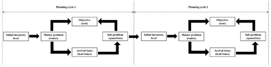
Figure 1.
A brief sketch for the problem (two planning cycles).
2.1. Problem Description
In this problem, we define a directed graph , where is a vertex set, and is an arc set. The vertex 0 and represent the same central depot. For each route, the starting vertex is 0 and the ending vertex is . The vertex set represents demand locations. For convenience, we further define and . The arc represents the shortest route between vertices i and j.
The planning horizon in each cycle is T. At the beginning of the planning cycle, check the initial inventory level . Then, a set of land vehicles and a set of aerial crafts depart from the central depot. They must return to the central depot before the end of the planning cycle. The unit transportation cost of a land vehicle is , and the unit transportation cost of an aerial craft is , where . Similarly, for each kind of vehicle, there are a capacity , and a fixed cost , .
We assume that the replenishment lead time of each demand location under each replenishment mode only considers the time consumption of transportation. We use and to represent the aerial and land replenishment lead time of each demand location, respectively. and represent the aerial and land replenishment quantity. Then we further define the lead time and replenishment quantity as 0 if the replenishment mode does not visit the demand location. For a demand location, the land replenishment mode may arrive earlier than the aerial mode due to the delivery order. Therefore, let and be defined as the lead time of the faster arrival replenishment method and the slower one when the demand location is replenished by both two modes. Similarly, and are faster and slower replenishment quantities, respectively. For a demand location, the inventory cost before the first replenishment arrival is not dependent on the replenishment quantity in the planning cycle, only depends on the initial inventory level, as shown in Figure 1. The initial inventory level is determined by the replenishment quantities of the last planning cycle. So, the objective should minimize the routing cost and the inventory cost from the beginning of this planning cycle to the fast replenishment arrival time in the next planning cycle. However, it is impossible to know the lead time information of the next planning cycle when planning the current cycle. Thus, we use the average fast lead time in the previous planning cycle to estimate it. This strategy is the planning horizon crossing.
Due to incomplete information, the distribution of demand is unknown. We assume demands are independent, and their values are in the positive symmetric interval , where is the estimated value of the demand and the maximum deviation of the demand. At the time point t, shelters deduct the demand between to t from the inventory held. If the available inventory does not meet the demand, it will have a backlog of demand to be met in the future, and a shortage cost will occur; otherwise, the on-holding inventory will be stored in the demand location to meet future demand, and lead to a holding cost. Each demand location has a unit holding cost h and a unit shortage cost s, where .
2.2. Notations
Notations used in the model are listed as follows:
Sets
V: Vertex set.
: Demand location set.
: .
: .
K: Land vehicle set.
A: Aerial vehicle set.
Parameters
: Time cost of transportation from i to j by land vehicles.
: Time cost of transportation from i to j by aerial vehicles.
: The unit cost of land transportation mode.
: The unit cost of aerial transportation mode.
: Fixed cost of land transportation mode.
: Fixed cost of aerial transportation mode.
: Capacity of a land vehicle.
: Capacity of an aerial vehicle.
: Initial inventory level of the demand location i at the beginning of the planning cycle.
: Average lead time for the first replenishment in the previous planning cycle.
T: Planning horizon of the planning cycle.
H: Inventory planning horizon, where .
Variables
: Arrival time of the demand location i replenished by vehicle k.
: Arrival time of the demand location i replenished by aerial vehicle a.
: Inventory level of the demand location i at time t.
: Replenishment quantity of the demand location i replenished by land vehicles.
: Replenishment quantity of the demand location i replenished by aerial vehicles.
: 1 if vehicle k of land transportation mode travels directly from vertex i to j; 0 otherwise.
: 1 if vehicle a of aerial transportation mode travels directly from vertex i to j; 0 otherwise.
: 1 if demand location i is assigned to route k; 0 otherwise.
: 1 if demand location i is assigned to route a; 0 otherwise.
2.3. Model
The objective function is the total cost in the planning cycle, including the transportation cost, and the inventory cost.
s.t.:
Constraint (2) is an inventory balance equation, where is the accumulated demand. {} is an indicator function, if , and ; constraints (3) and (4) guarantee the replenishment quantity is zero if no replenishment in the planning cycle; constraints (5) and (6) are used to determine the arrival time which equals to the replenishment lead time of demand locations, and it also eliminates subtours; constraints (7) and (8) guarantee that each demand location can only be replenished no more than once by each transportation mode; constraints (9) and (10) are assignment constraints; equations (11) and (12) are flow conservation constraints; and (13)–(20) are non-negativity and integrity of variables constraints.
3. Methodology
Under the rolling horizon framework, multi-period problems can be solved by following procedures. Firstly, set and solve the single-period model in the first planning cycle. Secondly, after the end of the planning cycle, initial inventory levels of the next planning cycle and the average lead time of the current planning cycle are revealed. Thirdly, update the inventory planning horizon H and roll the planning horizon to repeat the procedures until the last planning cycle. Note that the inventory planning horizon H will reset to T at the last planning cycle.
For the model proposed in Section 2.3, constraint (2) is non-linear and couples variables of replenishment quantities and lead times, which is hard to be solved. We decouple it into a master problem and a set of sub-problems. The sub-problem is an inventory problem. For any demand location, the sub-problem can be formulated as follows:
For the sub-problem, y and l are exogenous variables, which is determined by the routing decision. We derive a closed-form solution in Section 3.2. Thus, the problem can be solved by following procedures. Firstly, given a set of replenishment routes, the lead time of each demand location is determined. Then the optimal replenishment quantities can be solved by sub-problems. Finally, check the capacity constraints and repeat these procedures.
3.1. Robust Counterpart of Sub-Problem
For any demand locations, we assume the uncertainty demand between and t with the following non-negative bounded box uncertainty set:
Let denote the inventory cost between and t, the robust counterpart of the inventory model can be formulated as the following three situations:
- 1.
- When a demand location is not replenished in the planning cycle, the inventory cost is
- 2.
- When a demand location is replenished by only one mode in the planning cycle, the inventory cost iswhere l is the lead time, and q is the replenishment quantity.
- 3.
- When a demand location is replenished by both two modes in the planning cycle, the inventory cost iswhere and are the faster and the slower replenishment lead time, respectively. Similarly, and are the faster and the slower replenishment quantity.
3.2. Closed-Form Solution for Replenishment Quantity
Given a set of replenishment routes, the lead time of each demand location is an exogenous variable for a sub-problem. In Section 3.1, a linear programming model for sub-problems is proposed. In this section, we further derive a closed-form solution for replenishment quantity. When and for any , the following proposition derives an approximate optimal solution under the continuous time condition.
Proposition 1.
For any demand under a box uncertainty set U, letthe robust optimal replenishment quantity satisfy:
- For any demand location i replenished by a single replenishment mode, the optimal replenishment quantity is
- For any demand location i replenished by two replenishment modes, the faster and slower optimal replenishment quantities areand
Appendix A is the proof of Proposition 1.
3.3. Adaptive Variable Neighborhood Search
The variable neighborhood search (VNS) algorithm uses a set of fixed sequence neighborhoods for search. However, this problem contains two replenishment modes, and changing the routes of one replenishment mode will affect the route selection of another mode. A fixed search sequence may produce a fixed search structure, resulting in insufficient diversity of solutions. In this section, an adaptive variable neighborhood search algorithm is proposed. Two customer pools for each mode to determine which demand location is not served by the replenishment mode in the planning cycle. The “inter-route” and “pool” operators are used in the shaking phase, and the “intra-route” operators are used in the variable neighborhood descent (VND) phase. An adaptive mechanism is developed to select the operator from the shaking neighborhoods set in the first phase. The AVNS heuristic is described as follows:
- 1.
- Algorithm framework
The algorithm begins with an initial solution which is generated randomly. At each iteration, a neighborhood solution is generated from the current solution by using a selected shaking operator. Five heuristics are employed in this phase: removal, insertion, exchange, swap, and relocation operators. Then a neighborhood solution is generated from by using the VND strategy. Three heuristics are employed in this phase: 2-Opt, Or-Opt, and 3-Opt operators. The current solution is updated by the simulated annealing (SA) acceptance criterion. At the end of each iteration, scores for shaking operators are updated by the improvement of the solution. A segment contains several iterations, and the select probability of shaking operators is updated at the end of each segment. These processes repeat until the termination criteria are satisfied.
- 2.
- Shaking operators
In the shaking phase, five operators are used. Removal and insertion operators are “pool” operators, which are used for one route to evaluate whether a demand location should be replenished. Let represent the objective value and the penalty of the solution S, we define the operation cost as . These two operators choose a replenishment mode randomly, then traverse their entire neighborhood of to select the lowest operation cost solution as . The removal operator removes a demand location from a route and puts the demand location into the pool accordingly to the replenishment mode. The insertion operator inserts a demand location from the pool accordingly to the replenishment mode into a route. Exchange, swap, and relocation operators are used for “inter-route”, which operates on two routes under the same replenishment mode. These three operators randomly select a solution as from their neighborhood. The exchange operator exchanges two segments of different routes randomly. The swap operator randomly chooses two different routes. Then an arc of each route is opened, and swap demand locations are after the breakpoint. The relocation operator randomly chooses a demand location from a route and inserts it into another route. The illustration of these operators is shown in Figure 2.
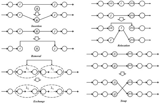
Figure 2.
Shaking operators.
- 3.
- VND operators
After the shaking phase, the “intra-route” operators with the VND strategy further optimize the affected routes. 2-Opt, Or-Opt, and 3-Opt operators are employed in this phase. These operators traverse their entire neighborhood of to select the lowest operation cost solution. Let i, j, and k are three positions in a route, where . The 2-Opt operator first opens the arc and the arc , then reverse the route between and k, and finally connect the arc and the arc . The Or-Opt operator opens arc , , and connect arcs , , . Similarly, the 3-Opt operator opens three arcs and connects them, respectively. However, the connection of this operator contains five situations, where two of them as the same as the 2-Opt and Or-Opt operators. So this operator only checks the other three situations. The illustration of these operators is shown in Figure 3.
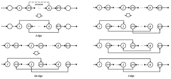
Figure 3.
VND operators.
- 4.
- SA acceptance criterion
We use an acceptance criterion based on the simulated annealing mechanism. For a current solution , a neighbour solution is accepted if and with probability otherwise. The current temperature is , where . The initial temperature is , and there is a cooling rate factor to decrease the temperature in each iteration, where .
- 5.
- Adaptive mechanism
The roulette-wheel mechanism determines the choice of which shaking operator is applied in each iteration. The probability for selection is based on the weight of each operator, which depends on its past performance, e.g., let be the weight of operator i, then operator j will be selected with probability . The weight is updated by scores. In each iteration, the applied shaking operator will gain a score. If the neighbour solution is better than the best solution , get ; if is better than the current solution , get ; if is no better than but accepted by the SA acceptance criterion, get ; if is not accepted, get 0. As mentioned before, the search progress is divided into segments, and each segment contains iterations. After the last iteration of each segment, shaking operators update their weights based on their scores. Let represent the sum of scores in the segment for shaking operator i, and is the number of times it is used in the segment. Then the weight of operator i in the next segment is updated by
where is called the reaction factor, controlling the adjustment speed. We set a protection threshold so that the weight will not be lower than to ensure that it is still may possible to select the operator with a lower weight in the later-stage iteration
- 6.
- Termination criteria
When the temperature reaches the cut-off threshold at each planning cycle, the iterations will cease.
- 7.
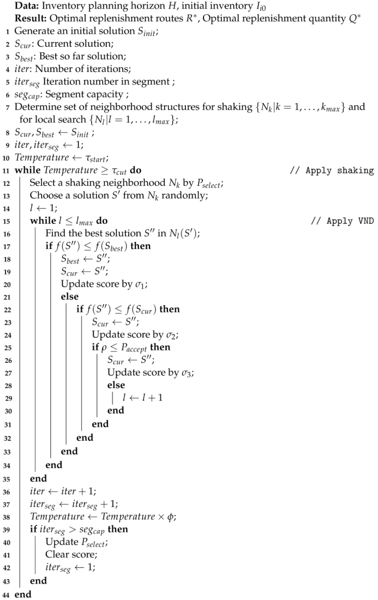
- Pseudocode
The pseudocode of the proposed AVNS heuristic shows in Algorithm 1:
| Algorithm 1: Adaptive variable neighborhood search |
 |
4. Numerical Experiments
This section provides the numerical experiments of the methodology proposed in Section 3. The AVNS algorithm is implemented on Python 3.9.0 and on a laptop with an Intel i7 1065G7 CPU processor and 16 GB RAM. All experiment results report in tables are the average of running 30 times, and outliers removed based on the PauTa criterion. Due to the absence of suitable benchmark instances available for the dual-sourcing inventory routing problem, we use a CVRP benchmark set and adjust some information. Nodes of Augerat’s CVRP benchmark instance set A is randomly generated in the range , where the first node is the central depot and the others are demand locations.
These numerical experiment parameters’ selection is based on the disaster relief background. We set the scale is 1:2 km. Trucks are land replenishment vehicles, and helicopters are aerial replenishment crafts. The land and aerial fleet size are set to be and , respectively. For a truck, the speed is 60 km/h, the fixed cost is 500, the using cost is 50/h, and the capacity is 5000. For a helicopter, the speed is 260 km/h, the fixed cost is 10,000, the using cost is 250/h, and the capacity is 2000. For a demand location, the average demand , the maximum deviation , the unit holding cost is , and the unit shortage cost is 2. The planning horizon at each planning cycle is 24 h, that . In Augerat’s benchmark instance set A, demands are generated in the interval . We use the demand information as the initial inventory level, where the volume times 20 to fit the number scale.
The score update parameters setting refers to Coelho et al. (2012), where , , and [40]. The starting temperature is set to and the cut-off temperature . The cooling rate is which yields roughly 3000 iterations at each planning cycle. The segment capacity and the reaction factor .
4.1. Algorithm Analyzes
The normalized weights of shaking operators are the selection probability of the operator in iterations. It can reflect the ability of an operator to find an acceptable/better solution than the current/best solution in the past iterations. As shown in Figure 4, normalized weights of five shaking operators are tested on three different instance scales. Removal and insertion operators outperform the other three operators. The normalized weights tend to be equal at the later-stage iterations. That is because as the temperature cools down and the iteration goes on, operators are more difficult to obtain scores. Their weight will gradually approach the protection threshold. This feature increases the diversity in searching at the later stage of iterations.
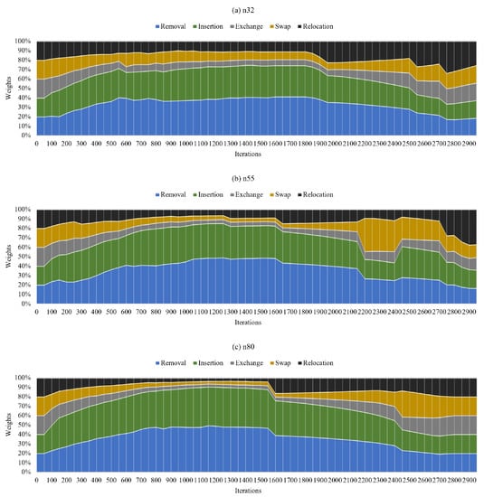
Figure 4.
Normalized weights of shaking operators.
However, the high weight can not entirely indicate that an operator can find a new best solution more effectively. The new acceptable solution also can obtain scores. So the ratio can reflect the ability of operators to find a new best solution, where is the percentage of an operator finding a new best solution times to the total best solution updated times, and is the percentage of an operator is used times to total iterations. Table 1 shows the ratio of shaking operators, which reflects the ability to find a new best solution in iterations.

Table 1.
Performance of shaking operators ( ratio).
The insertion operator shows the most effective ability to find new best solutions, whereas the exchange and swap operators demonstrate the least impressive results. However, removal and insertion operators traverse their entire neighborhood and select the lowest operation cost solution, instead of exchange, swap, and relocation operators selecting randomly. The removal and insertion operators are employed to evaluate if a demand location needs to be replenished, which is much like the “destroy–repair” strategy in the adaptive large neighborhood search algorithm. The other three operators provide diversity, similar to the shaking strategy in traditional VNS. The results of Figure 4 and Table 1 show that, although the weights of exchange, swap, and relocation operators are much lower than removal and insertion operators, the ratio of them are 0.30, 0.29, and 0.42, respectively. That means these three operators also effectively find new best solutions by providing diversity.
4.2. Model Analyzes
The single-period model under the rolling horizon framework is tested on all instances with three and seven planning cycles, respectively. We first study the robust solution and the deterministic solution on three planning cycles, where the robust solution is proposed by this work and the deterministic solution is solved by the average demands . Then the planning horizon crossing strategy is studied on instances with three and seven planning cycles. All gaps are calculated by
Table 2 shows the total cost of the robust solution and the deterministic solution when the real demands are or . The baseline is the robust solution. The gap between the robust solution and the deterministic solution when the real demands are is only . This gap is so small that we can hardly use more times experiments to exclude the influence of solution errors on the results. Because the solution is solved by the meta-heuristic algorithm and we cannot evaluate the gap between the obtained best solution and the optimal solution. It can explain why the robust solution is better than the deterministic solution in a few instances. When the real demands are the worst case (), the robust solution outperforms the deterministic solution on average.
Table 2.
Performance of robust solution under mean/maximum demand (3 cycles).
To evaluate the performance of our planning horizon crossing strategy, we test with and without this strategy on instances with three planning cycles and seven planning cycles. The baseline is the solution with planning horizon crossing strategy. Note that the planning horizon in the first and the last planning cycle are not crossing (). As shown in Table 3, the gap between the model with and without planning horizon crossing in three cycles and seven cycles are and , respectively. The result shows that the planning horizon crossing strategy can balance short-term decisions and long-term decisions, and reduce the out-of-stock cost before replenishment arrives in each planning cycle.
Table 3.
Comparing the model with/without planning horizon crossing.
5. Discussion
This study focuses on a novel inventory routing problem in which the lead time is dependent on the routing and has two modes of replenishment. Considering the transportation time in the lead time is of great significance for application scenarios with high timeliness requirements. For example, in emergency rescue, the central depot replenishes materials to shelters, and fresh food retailers replenish goods from the central depot to the front warehouse, etc. Supply of goods to demand locations more precisely can reduce waste and contribute to sustainability.
A robust model and an adaptive variable neighborhood search algorithm are proposed for the problem. There are five attractive features of our work: (1) the joint decision on inventory and transportation is investigated by considering replenishment-route-dependent lead time, which can better highlight the relationship between the arrival time and the related replenishment quantity; (2) a robust optimization model based on the rolling horizon framework is proposed, which is more appropriate to describe the features of the application scenarios under uncertainty, such as emergency logistics and perishable goods supply chains. (3) A closed-form optimal solution of replenishment quantity is derived under the box uncertainty set. (4) A planning horizon crossing strategy is proposed for balancing short-term decisions and long-term decisions in the rolling horizon framework. (5) A novel shaking stage of the adaptive variable neighborhood search algorithm is developed.
Numerical experiments study the proposed model and algorithm on a modified benchmark instance set. The robust solution is only worse than the deterministic solution when the demand is the predicted mean. On the other hand, when the demand is the worst case, the robust solution is better than the deterministic solution. It shows that our robust model can greatly reduce the effect of uncertainty at a very low cost. The planning horizon crossing strategy is effective and can save costs. The three cycles and seven cycles experiments show the planning horizon crossing strategy can save and costs than without it. For shaking operators in the AVNS algorithm, the insertion operator outperforms the others, and the ratio is . The ratio of removal, exchange, swap, and relocation operators are , , , and , respectively. It shows the insertion operator has the best performance of the ability to find new best solutions in iterations.
As with any research, ours begs for further extensions. Box uncertainty set is too conservative, other more novel uncertainty performs better on overcoming over-conservativeness. However, the closed-form solution for more complex uncertainty sets is a challenge. The rolling horizon framework is solved multi-period problems as a multi-stage decision-making problem by rolling planning horizon. Adjustable robust optimization is a methodology for multi-stage optimization. We will introduce adjustable robust optimization to our problem in future research. Compared with other articles that focus on the timeliness of replenishment, this paper introduces air–land transportation into the inventory routing problem to avoid the shortcomings that only use land transportation, such as road congestion or road damage after disasters. The adjacency matrix coefficient can reflect these situations. However, the model proposed in this paper cannot reflect the road congestion changes over time, and the dynamic model combined with real-time data will be a challenge.
Author Contributions
Conceptualization, W.Z.; methodology, W.Z. and H.Z.; software, W.Z.; validation, W.Z.; formal analysis, W.Z.; investigation, W.Z.; resources, W.Z.; data curation, W.Z.; writing—original draft preparation, W.Z.; writing—review and editing, W.Z. and H.Z.; supervision, H.Z.; funding acquisition, H.Z. All authors have read and agreed to the published version of the manuscript.
Funding
This research was funded by the National Natural Science Foundation of China, grant number 71971011.
Institutional Review Board Statement
Not applicable.
Informed Consent Statement
Not applicable.
Data Availability Statement
Publicly available datasets were analyzed in this study. The test set can be found at http://vrp.galgos.inf.puc-rio.br/index.php/en/ (accessed on 16 January 2023). The source code of the proposed AVNS algorithm can be found at https://github.com/WeberZheng/AVNS (accessed on 16 January 2023).
Conflicts of Interest
The authors declare no conflict of interest.
Abbreviations
The following abbreviations are used in this manuscript:
| AVNS | Adaptive variable neighborhood search |
| VNS | Variable neighborhood search |
| VND | Variable neighborhood descent |
| VIM | Vendor-managed inventory |
| IRP | Inventory routing problem |
| SA | Simulated annealing |
Appendix A. Proof
Proof of Proposition 1.
For a demand location, the inventory cost before the replenishment arrival is not affected by the replenishment quantity, it only depends on the initial inventory level. So the sub-problem is determining replenishment quantities to minimize the inventory cost after the replenishment arrival.
If the demand location is replenished, there are two situations:
- The demand location is replenished by one replenishment mode.If the initial inventory is enough, whereLet , the optimal replenishment quantity is 0 whenIf there is a turning point between the replenishment arrival time and the inventory planning horizon H. Where the inventory cost is from the holding cost turning to the shortage cost under the worst case. The turning point and the replenishment quantity q satisfy:Then,For any replenishment lead time l, the inventory cost after the replenishment isThe optimal replenishment quantity isThe closed-form solution for optimal replenishment quantity is
- The demand location is replenished by both two replenishment modes.If the initial inventory is enough before the slower replenishment arrival, whereThe optimal faster replenishment quantity is 0 whenSimilarly, the optimal slower replenishment quantity is 0 whenFor the faster arrival replenishment, if , there is a turning point between the twice replenishment.For any replenishment lead time , the inventory cost between the faster and the slower replenishment arrival time isThe closed-form solution for the faster replenishment quantity isFor the slower arrival replenishment, if , there is a turning point between the slower replenishment arrival time and the inventory planning horizon H.For any replenishment lead time , the inventory cost after the slower replenishment arrival isThe closed-form solution for the slower replenishment quantity is
□
References
- Comi, A. A modelling framework to forecast urban goods flows. Res. Transp. Econ. 2020, 80, 100827. [Google Scholar] [CrossRef]
- Bell, W.J.; Dalberto, L.M.; Fisher, M.L.; Greenfield, A.J.; Jaikumar, R.; Kedia, P.; Mack, R.G.; Prutzman, P.J. Improving the distribution of industrial gases with an on-line computerized routing and scheduling optimizer. Interfaces 1983, 13, 4–23. [Google Scholar] [CrossRef]
- Waller, M.; Johnson, M.E.; Davis, T. Vendor-managed inventory in the retail supply chain. J. Bus. Logist. 1999, 20, 183. [Google Scholar]
- Dror, M.; Ball, M.; Golden, B. A computational comparison of algorithms for the inventory routing problem. Ann. Oper. Res. 1985, 4, 1–23. [Google Scholar] [CrossRef]
- Çankaya, E.; Ekici, A.; Özener, O.Ö. Humanitarian relief supplies distribution: An application of inventory routing problem. Ann. Oper. Res. 2019, 283, 119–141. [Google Scholar] [CrossRef]
- Moin, N.H.; Salhi, S. Inventory routing problems: A logistical overview. J. Oper. Res. Soc. 2007, 58, 1185–1194. [Google Scholar] [CrossRef]
- Coelho, L.C.; Cordeau, J.F.; Laporte, G. Thirty years of inventory routing. Transp. Sci. 2014, 48, 1–19. [Google Scholar] [CrossRef]
- Shaabani, H. A literature review of the perishable inventory routing problem. Asian J. Shipp. Logist. 2022, 38, 143–161. [Google Scholar] [CrossRef]
- Chao, C.; Zhihui, T.; Baozhen, Y. Optimization of two-stage location–routing–inventory problem with time-windows in food distribution network. Ann. Oper. Res. 2019, 273, 111–134. [Google Scholar] [CrossRef]
- Imran, M.; Habib, M.S.; Hussain, A.; Ahmed, N.; Al-Ahmari, A.M. Inventory routing problem in supply chain of perishable products under cost uncertainty. Mathematics 2020, 8, 382. [Google Scholar] [CrossRef]
- Alvarez, A.; Cordeau, J.F.; Jans, R.; Munari, P.; Morabito, R. Formulations, branch-and-cut and a hybrid heuristic algorithm for an inventory routing problem with perishable products. Eur. J. Oper. Res. 2020, 283, 511–529. [Google Scholar] [CrossRef]
- Daroudi, S.; Kazemipoor, H.; Najafi, E.; Fallah, M. The minimum latency in location routing fuzzy inventory problem for perishable multi-product materials. Appl. Soft Comput. 2021, 110, 107543. [Google Scholar] [CrossRef]
- Harahap, A.Z.M.K.; Rahim, M.K.I.A. A single period deterministic inventory routing model for solving problems in the agriculture industry. J. Appl. Sci. Eng. 2022, 25, 945–950. [Google Scholar] [CrossRef]
- Li, M.; Wang, Z.; Chan, F.T. An inventory routing policy under replenishment lead time. IEEE Trans. Syst. Man Cybern. Syst. 2016, 47, 3150–3164. [Google Scholar] [CrossRef]
- Dror, M.; Ball, M. Inventory/routing: Reduction from an annual to a short-period problem. Nav. Res. Logist. NRL 1987, 34, 891–905. [Google Scholar] [CrossRef]
- Coelho, L.C.; Laporte, G. The exact solution of several classes of inventory-routing problems. Comput. Oper. Res. 2013, 40, 558–565. [Google Scholar] [CrossRef]
- Federgruen, A.; Zipkin, P. A combined vehicle routing and inventory allocation problem. Oper. Res. 1984, 32, 1019–1037. [Google Scholar] [CrossRef]
- Jaillet, P.; Bard, J.F.; Huang, L.; Dror, M. Delivery cost approximations for inventory routing problems in a rolling horizon framework. Transp. Sci. 2002, 36, 292–300. [Google Scholar] [CrossRef]
- Sakiani, R.; Seifi, A.; Khorshiddoust, R.R. Inventory routing and dynamic redistribution of relief goods in post-disaster operations. Comput. Ind. Eng. 2020, 140, 106219. [Google Scholar] [CrossRef]
- SteadieSeifi, M.; Dellaert, N.; Van Woensel, T. Multi-modal transport of perishable products with demand uncertainty and empty repositioning: A scenario-based rolling horizon framework. EURO J. Transp. Logist. 2021, 10, 100044. [Google Scholar] [CrossRef]
- Archetti, C.; Bertazzi, L.; Laporte, G.; Speranza, M.G. A branch-and-cut algorithm for a vendor-managed inventory-routing problem. Transp. Sci. 2007, 41, 382–391. [Google Scholar] [CrossRef]
- Hvattum, L.M.; Løkketangen, A.; Laporte, G. Scenario tree-based heuristics for stochastic inventory-routing problems. Informs J. Comput. 2009, 21, 268–285. [Google Scholar] [CrossRef]
- Huang, S.H.; Lin, P.C. A modified ant colony optimization algorithm for multi-item inventory routing problems with demand uncertainty. Transp. Res. Part E Logist. Transp. Rev. 2010, 46, 598–611. [Google Scholar] [CrossRef]
- Alvarez, A.; Cordeau, J.F.; Jans, R.; Munari, P.; Morabito, R. Inventory routing under stochastic supply and demand. Omega 2021, 102, 102304. [Google Scholar] [CrossRef]
- Soyster, A.L. Convex programming with set-inclusive constraints and applications to inexact linear programming. Oper. Res. 1973, 21, 1154–1157. [Google Scholar] [CrossRef]
- Mamani, H.; Nassiri, S.; Wagner, M.R. Closed-form solutions for robust inventory management. Manag. Sci. 2016, 63, 1625–1643. [Google Scholar] [CrossRef]
- Levi, R.; Pál, M.; Roundy, R.O.; Shmoys, D.B. Approximation algorithms for stochastic inventory control models. Math. Oper. Res. 2007, 32, 284–302. [Google Scholar] [CrossRef]
- Levi, R.; Janakiraman, G.; Nagarajan, M. A 2-approximation algorithm for stochastic inventory control models with lost sales. Math. Oper. Res. 2008, 33, 351–374. [Google Scholar] [CrossRef]
- Sun, J.; Van Mieghem, J.A. Robust dual sourcing inventory management: Optimality of capped dual index policies and smoothing. Manuf. Serv. Oper. Manag. 2019, 21, 912–931. [Google Scholar] [CrossRef]
- Tagaras, G.; Vlachos, D. A periodic review inventory system with emergency replenishments. Manag. Sci. 2001, 47, 415–429. [Google Scholar] [CrossRef]
- Musolino, G.; Polimeni, A.; Vitetta, A. Freight vehicle routing with reliable link travel times: A method based on network fundamental diagram. Transp. Lett. 2018, 10, 159–171. [Google Scholar] [CrossRef]
- Comi, A.; Polimeni, A. Estimating path choice models through floating car data. Forecasting 2022, 4, 525–537. [Google Scholar] [CrossRef]
- Croce, A.I.; Musolino, G.; Rindone, C.; Vitetta, A. Traffic and Energy Consumption Modelling of Electric Vehicles: Parameter Updating from Floating and Probe Vehicle Data. Energies 2022, 15, 82. [Google Scholar] [CrossRef]
- Russo, F.; Rindone, C. Regional transport plans: From direction role denied to common rules identified. Sustainability 2021, 13, 9052. [Google Scholar] [CrossRef]
- Zhang, M.; Yu, J.; Zhang, Y.; Yu, H. Programming model of emergency scheduling with combined air–ground transportation. Adv. Mech. Eng. 2017, 9, 1687814017739512. [Google Scholar] [CrossRef]
- Sacramento, D.; Pisinger, D.; Ropke, S. An adaptive large neighborhood search metaheuristic for the vehicle routing problem with drones. Transp. Res. Part C Emerg. Technol. 2019, 102, 289–315. [Google Scholar] [CrossRef]
- Zheng, W.; Zhou, H. Routing problem with multiple transportation modes considering road damage. In Proceedings of the 2018 International Conference on Computer Modeling, Simulation and Algorithm (CMSA 2018), Beijing, China, 22–23 April 2018; Atlantis Press: Amsterdam, The Netherlands, 2018; pp. 250–253. [Google Scholar] [CrossRef]
- Mahjoob, M.; Fazeli, S.S.; Milanlouei, S.; Tavassoli, L.S.; Mirmozaffari, M. A modified adaptive genetic algorithm for multi-product multi-period inventory routing problem. Sustain. Oper. Comput. 2022, 3, 1–9. [Google Scholar] [CrossRef]
- Zheng, W.; Zhou, H. Robust inventory routing problem with replenishment lead time. In Proceedings of the 2019 IEEE International Conference on Industrial Engineering and Engineering Management (IEEM), Macao, China, 15–18 December 2019; IEEE: Piscataway, NJ, USA, 2019; pp. 825–829. [Google Scholar] [CrossRef]
- Coelho, L.C.; Cordeau, J.F.; Laporte, G. The inventory-routing problem with transshipment. Comput. Oper. Res. 2012, 39, 2537–2548. [Google Scholar] [CrossRef]
- Hernández-Pérez, H.; Rodríguez-Martín, I.; Salazar-González, J.J. A hybrid heuristic approach for the multi-commodity pickup-and-delivery traveling salesman problem. Eur. J. Oper. Res. 2016, 251, 44–52. [Google Scholar] [CrossRef]
- Mirzapour Al-e hashem, S.M.J.; Rekik, Y. Multi-product multi-period Inventory Routing Problem with a transshipment option: A green approach. Int. J. Prod. Econ. 2014, 157, 80–88. [Google Scholar] [CrossRef]
- Shen, Q.; Chu, F.; Chen, H. A Lagrangian relaxation approach for a multi-mode inventory routing problem with transshipment in crude oil transportation. Comput. Chem. Eng. 2011, 35, 2113–2123. [Google Scholar] [CrossRef]
- Agra, A.; Christiansen, M.; Wolsey, L. Improved models for a single vehicle continuous-time inventory routing problem with pickups and deliveries. Eur. J. Oper. Res. 2022, 297, 164–179. [Google Scholar] [CrossRef]
- Li, C.; Gong, L.; Luo, Z.; Lim, A. A branch-and-price-and-cut algorithm for a pickup and delivery problem in retailing. Omega 2019, 89, 71–91. [Google Scholar] [CrossRef]
Disclaimer/Publisher’s Note: The statements, opinions and data contained in all publications are solely those of the individual author(s) and contributor(s) and not of MDPI and/or the editor(s). MDPI and/or the editor(s) disclaim responsibility for any injury to people or property resulting from any ideas, methods, instructions or products referred to in the content. |
© 2023 by the authors. Licensee MDPI, Basel, Switzerland. This article is an open access article distributed under the terms and conditions of the Creative Commons Attribution (CC BY) license (https://creativecommons.org/licenses/by/4.0/).