Abstract
Stereophonic audio devices employ two loudspeakers and two microphones in order to create a bidirectional sound effect. In this context, the stereophonic acoustic echo cancellation (SAEC) setup requires the estimation of four echo paths, each one corresponding to a loudspeaker-to-microphone pair. The widely linear (WL) model was proposed in recent literature in order to simplify the handling of the SAEC mathematical model. Moreover, low complexity recursive least- squares (RLS) adaptive algorithms were developed within the WL framework and successfully tested for SAEC scenarios. This paper proposes to apply a data-reuse (DR) approach for the combination between the RLS algorithm and the dichotomous coordinate descent (DCD) iterative method. The resulting WL-DR-RLS-DCD algorithm inherits the convergence properties of the RLS family and requires an amount of mathematical operations attractive for practical implementations. Simulation results show that the DR approach improves the tracking capabilities of the RLS-DCD algorithm, with an acceptable surplus in terms of computational workload.
1. Introduction
The standard acoustic echo cancellation (AEC) setup is used by communication terminals comprised of one loudspeaker and one microphone. The AEC process employs an adaptive filter to estimate an unknown impulse response, which generates undesired replicas of the loudspeaker signal [1,2,3]. The goal is to eliminate the unknown system’s output (or the echo) contribution from the mix of signals captured by the microphone, which is situated in the same room [1,4,5,6,7]. The corresponding unknown system identification configuration uses as input the loudspeaker signal, with the microphone’s input as a reference. From the microphone contributions, an echo estimate is subtracted, and the resulting signal is sent to the interlocutor, ideally without any unwanted acoustic replicas.
When the communication terminal consists of N loudspeakers with M microphones, the number of possible echo paths is given by the value [4,8,9,10]. The stereophonic communication terminal represents the minimal configuration which can provide the impression of audio directionality, having . In order to perform the stereophonic AEC (SAEC), we must take into consideration that each loudspeaker-to-microphone pair can generate unwanted acoustic replicas. Correspondingly, two input (loudspeaker) signals with two microphone signals, are used in four AEC-type system identification setups in order to estimate four corresponding unknown impulse responses [4,8,11,12,13]. Additionally, compared to the single channel scenarios, the SAEC process is also hindered by the existing correlation between the two acoustic channels, which might not generate unique solutions when using adaptive algorithms [8,9,14,15,16,17]. In the recent literature, the solution to the problem represented by the coherence between the acoustic channels has been approached by employing a pre-distortion block, which mitigates the correlation with some cost in terms of signal quality [4,5,9,18].
In [5,18], the widely linear (WL) model was introduced in order to improve the handling of the SAEC framework when employing several types of adaptive filters. It groups the four adaptive filters and multiple real valued variables into a single adaptive filter and fewer complex valued variables (CRVs). Moreover, the WL approach also opened the way for other various developments proposed for SAEC systems, such as improved behaviour when working in low signal-to-noise ratio (SNR) conditions [19]. Although considerable effort was invested in enhancing robustness features, the SAEC setup interpreted using the WL framework leaves more room for applying developments which has proved to be successful for other configurations employing adaptive systems.
Among the essential performance indicators for any adaptive algorithm in AEC/SAEC scenarios (i.e., system identification setups) [1,4,20], the tracking speed represents the capacity of following any changes that might occur in the unknown echo paths. The current adaptive systems in the industry employ algorithms from the least-mean-square (LMS) family for most practical applications [1]. The LMS methods have the advantage of delivering satisfactory performance with a relatively limited arithmetic effort with respect to other potential solutions. However, they provide poor results when working with highly correlated input signals (such as speech) in terms of tracking speed and accuracy at steady state (i.e., when convergence is achieved).
Consequently, due to their capabilities of reducing the correlation of input signals and generating superior tracking performances, the recursive least-squares (RLS) family of algorithms is the subject to considerable research. They are also known for their excessively costly arithmetic workloads, which make them prohibitive for practical applications. However, a successful attempt at mitigating this problem is the combination between the exponentially weighted RLS and the dichotomous coordinate descent (DCD) iterations [5,21,22]. The RLS-DCD algorithm generates performance similar to classical RLS versions, such as the one employing the matrix inversion lemma [1]. The RLS-DCD replaces the classical matrix inversion problem with an auxiliary system of equations and exploits the time-shift nature of the input data in order to generate a solution using only additions and bit shifts. The overall complexity corresponding to the RLS-DCD algorithm is proportional to the adaptive filter’s length multiplied by a small factor (in terms of multiplications and additions).
In this paper, we improve the tracking capabilities of the RLS-DCD algorithm working within the WL framework by employing the recently introduced data-reuse (DR) approach for adaptive algorithms from the RLS family [23,24]. The DR methodology is based on performing multiple filter updates using the same input data (i.e., in the same adaptive filter iteration). In the recent literature, it proved to generate superior performance for other RLS versions, with the cost of some extra arithmetic effort when used for real valued adaptive filters in system identification scenarios [23]. Simulation results will demonstrate that the namely WL-DR-RLS-DCD has increased tracking capabilities even when identifying long impulse responses and using highly correlated input signals, such as speech sequences. The complexity analysis will also reveal that the proposed method requires acceptable hardware resources, and it is a suitable candidate for practical applications in SAEC scenarios with long acoustic paths.
The remainder of this paper is organized as follows. In Section 2, the SAEC system configuration based on the WL model is introduced. Section 3 describes the complex valued WL-RLS-DCD algorithm for SAEC scenarios, and Section 4 introduces a new version of the presented adaptive method based on the DR approach with improved tracking capabilities. Simulation results are discussed in Section 5. Several relevant aspects are discussed in Section 6, and a few conclusions are drawn in Section 7 based on the theoretical contributions in the presented simulations.
2. System Model
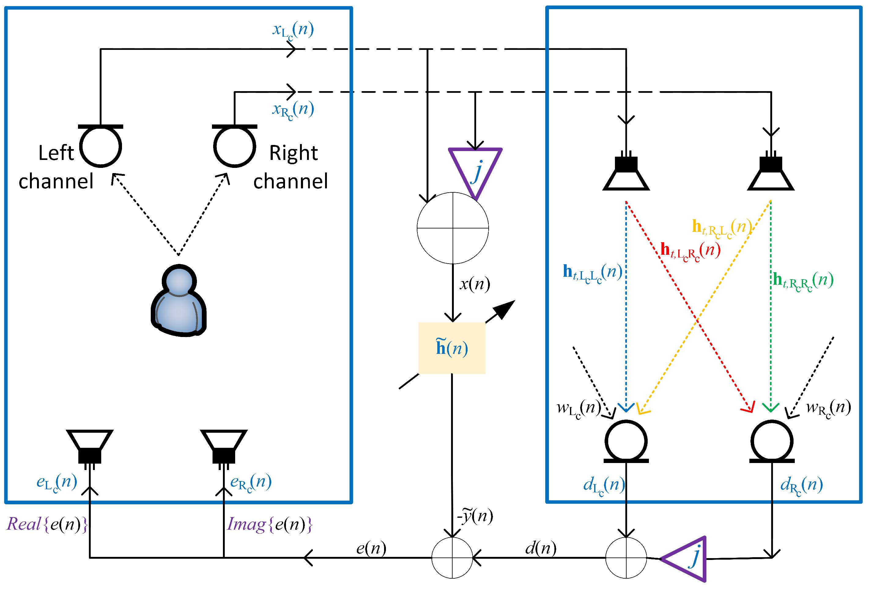
For the SAEC configuration (see Figure 1), we refer to the acoustic channels as the left () and the right one (). We employ the discrete time index n to denote the input (loudspeaker) signals as and . They can be used to express two vectors comprising the most recent L input samples for each channel as [4]:
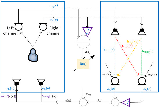
Figure 1.
The WL model for SAEC systems.
Moreover, we combine the four loudspeaker-to-microphone echo path impulse responses of length L (denoted by the vectors , , , and ) to write the echo contributions corresponding to the stereophonic channels [4]:
where superscript T denotes the transpose operator. Consequently, the microphone signals can be expressed as [4]:
where and represent environmental noise signals, which are uncorrelated with and .
The WL model combines the previously introduced real random variables into fewer CRVs in order to improve the handling of the SAEC setup. The signals associated with the inputs and the outputs of the unknown echo paths can be paired using the notation into:
Moreover, the four unknown impulse responses can be combined into
with the purpose of obtaining the complex valued forms [4]
and express the output complex signal as
where the superscripts H and * denote the transpose-conjugate and conjugate operators, respectively, and
Consequently, the complex vectors from (11) and (12) can be concatenated to obtain the complex valued vector comprising the information corresponding to the coefficients of the four unknown impulse responses
and a corresponding input vector can be defined as
Finally, by also expressing the complex valued noise as
the microphone signals corresponding to the left and right channels can be written as:
The error signal can now be expressed as
where is the estimate of the complex valued system’s output computed using the adaptive filter’s set of coefficients (which approximates ).
The described framework improves the handling of SAEC scenarios using adaptive algorithms. Moreover, it favors the development of corresponding new features by re-casting four unknown system identification problems into a single one. The two-input/two-output system with real random variables is viewed as a single-input/single-output system with CRVs.
3. WL-RLS-DCD
For the RLS family of adaptive algorithms employed in SAEC scenarios with the WL framework, the vectors from (16) and (17) are interleaved instead of concatenated (as it was presented in the previous section). However, the new formulations do not affect the definition of the complex reference signal [4,5].
Firstly, the vector comprising the input samples from (14) and (17) is redefined to reflect the new positioning of the complex valued samples and their transpose-conjugate counterparts. Consequently, we write:
In a similar manner, the elements of (11) and (12) are also interleaved in order to express the new complex valued impulse response to be estimated [4,5]:
where and , with , are the elements of the vectors and , respectively.
When employing the least-squares approach to generate the complex valued estimate vector of , the corresponding cost function is written using (22), (23), and the complex observation as:
where denotes the forgetting factor, which controls the memory of the algorithm (i.e., values closer to one increase the adaptive filter’s performance in steady state, while low values for improve the tracking capabilities of the system) [1,4]. When performing the minimization of the error criterion, two new notations are introduced, i.e., the estimate of the correlation matrix
and the cross-correlation vector between the complex input signal and the desired signal
Thus, the solution for the normal set of equations
leads to the straight-forward expression for the adaptive filter’s coefficients:
The direct approach for computing has a complexity of , which is too costly for practical implementations, such as the ones for SAEC configurations. In acoustic applications, the number of filter coefficients can easily be in the range of hundreds or even thousands. Other classical solutions, such as the one based on Woodburry’s identity (also known as the matrix inversion lemma [1,4]), provide an alternative to (28) with a complexity . However, the required amount of arithmetic operations is still prohibitive for most computer chips and would considerably increase device prices, power consumption, etc.
In this context, the combination between the exponentially weighted RLS adaptive algorithm and the DCD iterations was proposed as a computationally efficient method, with a complexity proportional to the adaptive filter’s length multiplied by a small number (the actual details will be discussed in the next paragraphs). The WL-RLS-DCD is accepted as a reliable algorithm in multiple types of configurations for acoustic echo cancellation, including for stereophonic communication setups [5,18,21].
The steps of the WL-RLS-DCD are described in Table 1, where we denoted by the first column of the matrix and by a small positive constant employed to initialize the correlation matrix in a non-singular form. The updates in Steps 1 and 2 can be performed by relying on the time-shift property of the input vector , which is also translated to . The upper-left sub-matrix of can be copied to the lower-right sub-matrix, and only the first two columns and first two rows must be computed. If we take into consideration that the matrix is Hermitian, the first two rows can be obtained from the first two columns. Moreover, for every pair of consecutive columns, starting with an odd position (e.g., column 1, column 3, etc.), the sets of values comprising one of the columns can also be found in the other column in a conjugate form, at a distance of ±1 row. Consequently, the only arithmetic operations necessary for updating can be employed for a single column (i.e., a set of values). The described methodology shows how the arithmetic complexity corresponding to Steps 1 and 2 from Table 1, which is apparently , can be kept to value proportional to (i.e., the filter’s length). Further possible optimizations, such as the option of storing only a part of the matrix, are up to the developers performing the hardware implementations and deciding on the associated compromises. The latter depend considerably on the value of L (i.e., the associated memory requirements versus the necessary extra logic elements required to exploit the time-shift properties).

Table 1.
WL-RLS-DCD Algorithm.
Steps 3 and 4 of the WL-RLS-DCD represent the standard filtering operation and the trivial computation of the error signal. In Step 5, the residual component is updated for the current time index by applying the forgetting factor to the so-called residual vector . The residual component is then employed in Step 6 as part of an auxiliary system of equations, which can be solved by exploiting the properties of the correlation matrix with the DCD iterations. Step 6 produces two sets of results. Firstly, the solution vector, denoted by , is used in Step 7 by adding it to the filter coefficients determined at the previous time index, thus generating the updated estimate of the unknown complex valued system. Secondly, the residual vector is computed to reflect the changes performed in the filter update process through . As can be noticed in Steps 5 and 6, the vector will be relevant at the next time index as part of the next DCD operation.
Table 2 shows a description of the DCD iterations with a leading element. It can be noted that is initialized with zeros values, and at the end of the entire DCD procedure, it represents the solution vector to a system which also comprises the matrix and the residual component .
Table 2.
Complex valued DCD iterations with a leading element at time index n.
The DCD algorithm works under the presumption that is comprised of complex values on all positions except the main diagonal, where all values are real positive numbers. Moreover, on the main diagonal, all values are statistically considerably higher than all other real or imaginary values in the rest of the matrix (in terms of absolute values). By exploiting this property, Step 1 of the algorithm chooses the position with the greatest absolute value in (all real and imaginary parts) and performs a comparison with its counterpart (i.e., same position) on the main diagonal of in order to determine if an update should be made in the solution vector. This approach is considered a behaviour because it searches for the most probable position where an update could be triggered for .
The parameters of the DCD iterations are the maximum expected amplitude H, the step size , the number of bits used for the numerical representation of the real and imaginary values comprising , and the maximum number of allowed updates . The value of H is usually chosen as a power of two (e.g., ), and it is used to initialize the value of the step size. Considering how the latter is updated in Step 2 of Table 2, this choice ensures that the multiplication operations performed with are equivalent to bit shifts.
In Step 1 of the DCD iterations, a search is performed amongst all real and imaginary parts comprising the vector in order to determine the maximum absolute value and its corresponding position. The target value is employed in Step 4 to decide if an update is triggered, by comparing it to the (real and positive) value situated on the corresponding position of the main diagonal of , which is scaled using the step size. If an update is decided, then the same position in the solution vector (i.e., ) is updated using and the sign of . The operation is equivalent to setting a bit in the binary representation of one of the real and imaginary values comprising the solution vector . Moreover, the coefficient update is always followed by another change in the vector on the same position p (Step 6). It is important to note that is initialized at the beginning of the DCD with the values comprising the residual component , and after the changes performed by the algorithm, it will represent the residual vector .
If the condition in Step 4 does not trigger an update, then a jump is made to Step 2, and the value of the step size is halved, making point to the next lesser significant bit possible. Such an operation can be performed until the algorithm reaches the least significant bit it can process (i.e., until ). Consequently, the algorithm can perform a total number of updates upper limited by (see the loop), or it can exit when it would need to perform updates in the solution vector equivalent to binary values smaller than the least significant bit used to represent the real and imaginary values comprising (Step 3). Due to the nature of the auxiliary system of equations, it is expected the WL-RLS-DCD will generate satisfactory performance with a small value of (less than 10, or comparable to it, for larger systems, with thousands of coefficients). In addition, it is natural to assume at this point that the value also denotes the number of bits used to represent the real and imaginary parts of the coefficients comprising the adaptive filter .
The overall complexity of the employed DCD algorithm (at any time index n) takes into account that bit shifts replace all potential multiplications, and only additions are employed. Moreover, a maximum number of update operations can be performed on the solution vector. The final number of modified coefficients (which are all initialized with 0) is expected to be much smaller than the filter’s length (i.e., ). In [5,21], it was demonstrated that the DCD iterations can generate performance similar to other classical RLS methods for values of smaller than 10. Consequently, the upper limit for the amount of additions is noted in Table 2.
Information regarding the arithmetic complexity of the WL-RLS-DCD is also displayed in Table 1, in terms of real valued multiplications and additions. For the DCD stage of the adaptive algorithm, we evaluated the most complex scenarios when the maximum number of allowed updates is employed. It can be noted that the amount of necessary multiplications is a small multiple of the complex valued adaptive filter’s length. The same conclusion can be drawn for the number of additions, which are combined with bit shifts in order to solve the auxiliary system of the equation in Step 6.
4. WL-DR-RLS-DCD
In the recent literature, for the process of determining from when employing RLS adaptive algorithms, the DR approach was introduced in order to improve their corresponding tracking speeds [23,24]. Correspondingly, in order to update the filter’s coefficients multiple times at the same time index n (i.e., for the same input data), Steps 3–7 from Table 1 will be run in a loop for a number of iterations (including the DCD method). We call the proposed algorithm the WL-DR-RLS-DCD, which is equivalent to the WL-RLS-DCD for .
For each of the DR iterations, the algorithm will determine a new solution vector , based on the same input data [i.e., and ] and add its contribution to the filter estimate accumulated with all previous DR iterations from time index n. The complex reference will remain the same for all the steps, as no updated value will be made available from outside the adaptive system. However, the error signal and the residual contribution will be updated accordingly and will go through stages. We will distinguish them using the notations and , with .
At the beginning of the DR process (i.e., for ), the form of the complex output signal remains the same as (18), corresponding to the estimate . For the next iterations (), the output is adjusted according to the new updates performed by the DCD, which leads to the analytical expression:
We denote the first complex output sample for time index n as
and we can recursively express the output for iterations as
Consequently, by using (21) and (31), the form of the complex valued error can also be recursively written as
The expression in (32) is relevant from an implementation point of view because when dealing with values of L specific to acoustic environments, most of the arithmetic costs for updating the complex error correspond to the computation of (the workload associated with the classical WL-RLS-DCD method). For the iterations corresponding to , we must take into account in (32) that a maximum amount of values are non-zero at each iteration in the corresponding solution vector . Therefore, all the rest of iterations require no more than complex multiplications, and the same number of complex additions, in order to accumulate them to the error signal.
For the residual elements associated with the DCD method, at each iteration of the DR process we consider that a residual component is used as input for each DCD run, and an associated residual vector is generated [besides ]. The DR approach creates a cycle, which comprises, for each iteration, updates performed for the error signal , then for the residual component , in order to prepare for the DCD run. The latter generates a solution vector and a residual vector , which will be used for updating the filter coefficients, and also in the next DR iteration, in order to repeat the same steps.
In a manner similar to , the update of must be split into two possible types of operations. Firstly, for (i.e., the first DR iteration at time index n), the update will employ the forgetting factor in order to perform the transition from . Secondly, for , is changed in order to reflect the error updates from (32) and the latest residual vector generated by the DCD algorithm. Consequently, we can write:
where is the residual vector determined by the last run of the DCD at time index .
Furthermore, we can also express the update process for the filter estimate as
where represents the last set of filter coefficients computed at the previous iteration of the adaptive algorithm. It can be noted that for a number of iterations , the updates described in (32)–(34) are each performed only for the first branch, which makes the WL-DR-RLS-DCD behave exactly as the WL-RLS-DCD algorithm.
The proposed adaptive algorithm is summarized in Table 3. It also comprises the corresponding information related to arithmetic workloads (in terms of real valued multiplications and additions). Just as in the case of the WL-RLS-DCD, we considered that counters with small values can be implemented as delay lines (i.e., bit shifts performed for binary arrays). The extra arithmetic effort determined by the DR approach (with respect to Table 1) is directly influenced by the number of iterations , which is expected to be a number lower than 10. As was already discussed in [23,24], the expected gain in terms of tracking speed becomes limited when increases beyond a certain value. Consequently, the overall complexity of the WL-DR-RLS-DCD remains proportional to the length of the complex valued filter multiplied by a small integer.
Table 3.
WL-DR-RLS-DCD algorithm.
5. Simulation Results
Simulations were performed in the context of SAEC using the WL framework. The input signal was filtered through two distinct real acoustic impulse responses in order to simulate the effect of the left and right channels and generate the samples and . The input signal source was chosen as a Gaussian noise filtered through an auto-regressive (AR) system with a single pole and a speech sequence [25].
In order to overcome the problem of the correlation between the sequences and , we employed the nonlinear pre-distortion approach presented in [4,18]. The method implies the addition of a specific level of distortion to the input signals, and , respectively, in order to obtain a unique solution. The namely half-wave rectifier generates two new signals using the expressions [4,9,18]
where the parameter controls the amount of nonlinearity. In practice, the stereo effect is considered not to be drastically affected for the range .
The performance of the proposed WL-DR-RLS-DCD algorithm has been validated in the context of the identification of the interleaved impulse response , with respect to the results provided by the version with DR iterations (i.e., the WL-RLS-DCD). The performance has been measured using the normalized misalignment, having the following expression in the WL context:
where denotes the norm [4].
The forgetting factor was chosen with the form , and the parameters specific to the DCD iterations were set to , and . For the simulations using an AR(1) sequence as input, the pole was set to . The four unknown echo paths are real measured acoustic impulse responses, which have been decimated in order to have the desired lengths (indicated in the caption of each figure). Finally, the SNR was experimentally set to 25 dB for all scenarios [4,5].
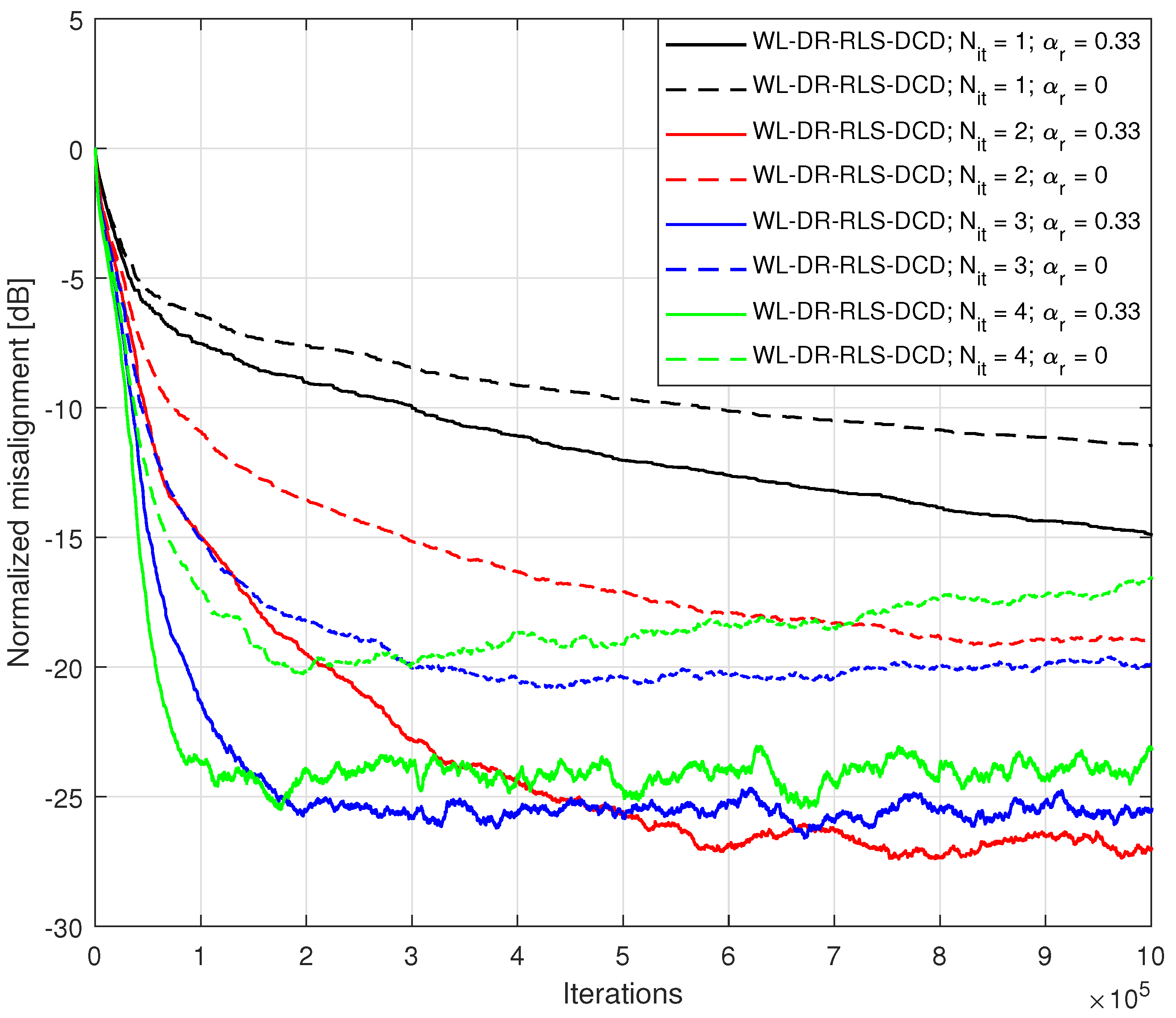
In Figure 2, we studied the performance of the proposed algorithm for different values of the DR parameter and for two values of the pre-distortion parameter: (A) (no pre-distortion is applied) and (B) ( pre-distortion used for the complex input signal). It can be noted that for every value of the performances corresponding to (B) are considerably superior to their counterparts from case (A). The mitigation of correlation between the real valued input signals associated with the two channels leads to better performance for the adaptive filter. For every value of , the gain in terms of normalized misalignment is at least 5 dB at steady state. Moreover, as the value of the parameter increases, so does the initial convergence speed of the WL-DR-RLS-DCD. The corresponding compromise is made with the associated extra arithmetic workload and a reduction in accuracy of the adaptive algorithm when steady state is reached. Finally, it can also be observed that with higher values of , the progress in terms of convergence speed becomes smaller, such that the corresponding gain tends to become capped.
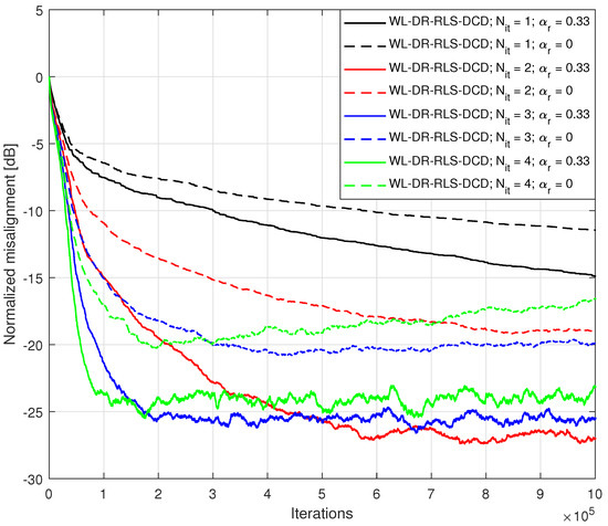
Figure 2.
Misalignment of the WL-DR-RLS-DCD algorithm for different values of . The input signal is an AR(1) sequence with the pole 0.95, and it is pre-distorted () or not pre-distorted at all (). The length of the four unknown impulse responses is and .
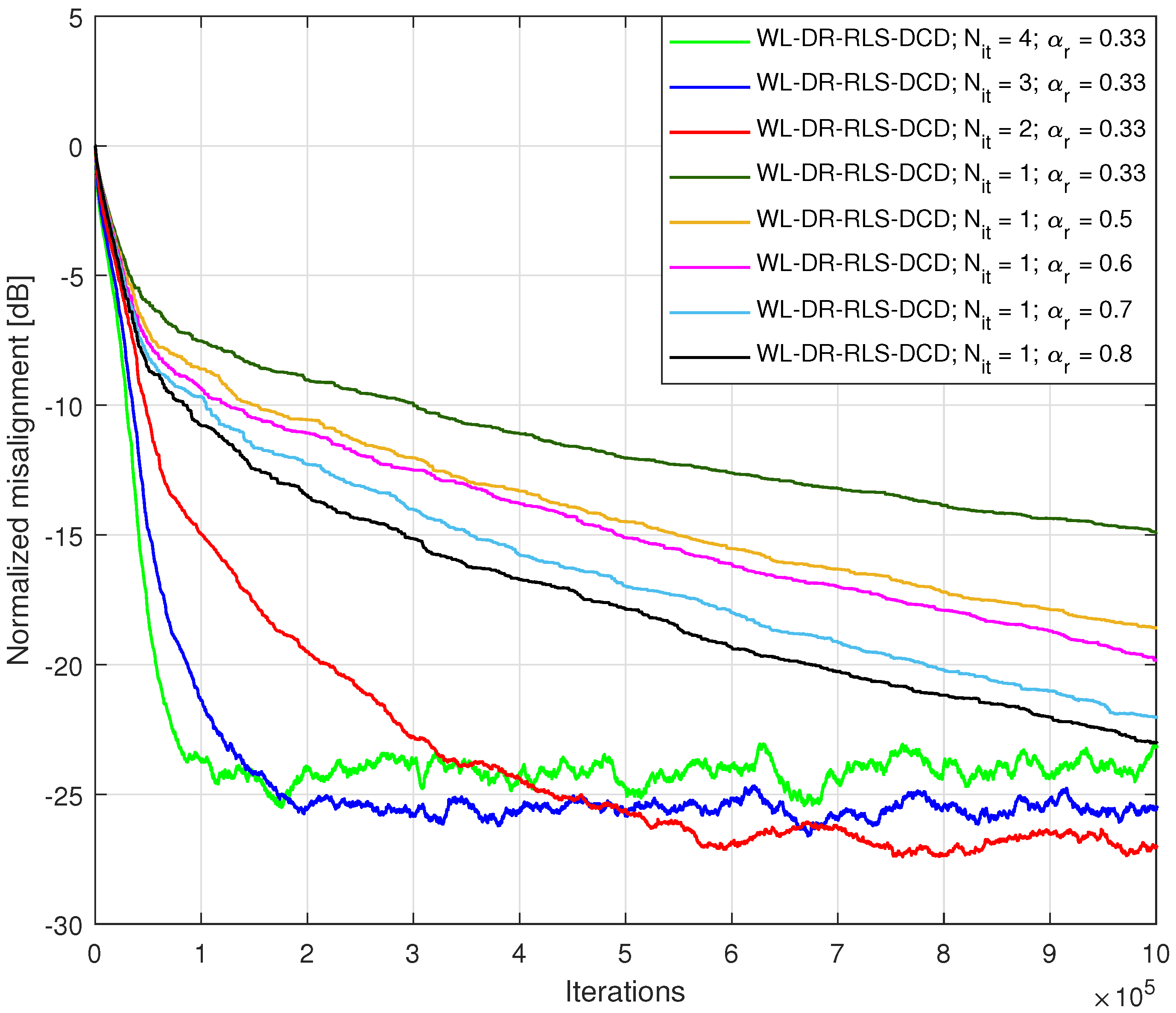
In Figure 3, we compare the performance of the WL-RLS-DCD for different values of with the WL-DR-RLS-DCD having . We increased the pre-distortion parameter above the recommended limit in order to analyze the possibility of compensating a high number of DR iterations and save extra costs in terms of arithmetic operations required by the WL-DR-RLS-DCD with higher values for . It can be noted that even the convergence speeds associated with values (i.e., when the stereo effect is altered) cannot match the misalignment performance of using and . All normalized misalignment curves corresponding to require more than iterations to reach steady state (i.e., around −25 dB), which exceeds the boundaries of the presented simulation interval.
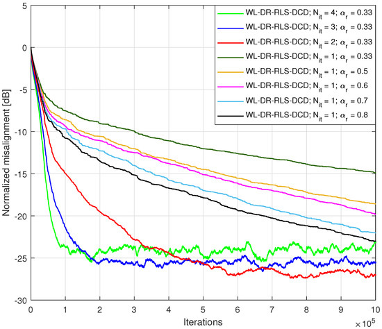
Figure 3.
Misalignment of the WL-DR-RLS-DCD algorithm for different values of and different values of the pre-distortion parameter . The input signal is an AR(1) sequence with the pole 0.95, and the length of the four unknown impulse responses is and .
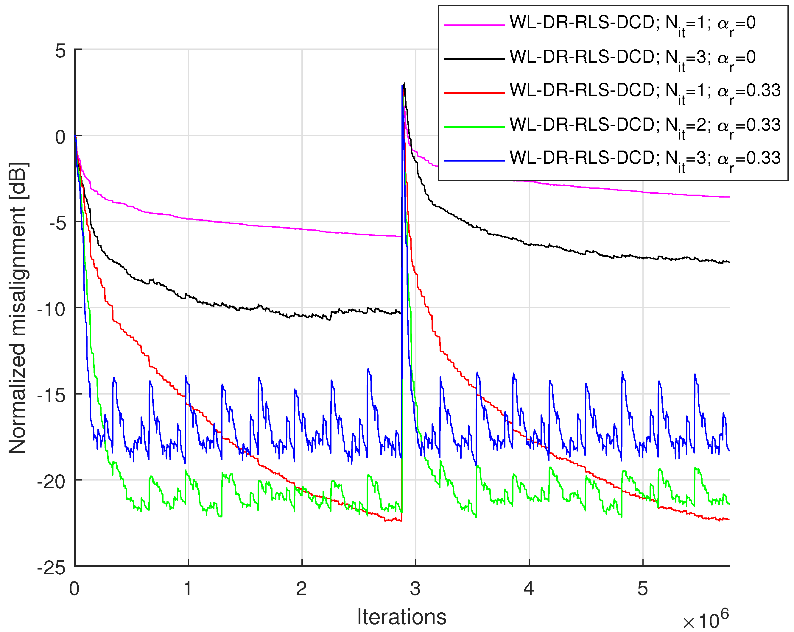
The last experiment is presented in Figure 4. The input signal is a speech sequence. The unknown impulse responses are longer than the ones employed in the previous scenarios and are changed after half of the simulation is completed by shifting them 25 positions to the right (tracking scenario). We compared the performances of the WL-DR-RLS-DCD for the same value of and different number of DR iterations. As a reference, we also added the corresponding results for the lowest and highest value of when the input signal is not pre-distorted. It can be noted that as the number of DR iterations increases, the tracking capabilities of the WL-DR-RLS-DCD improve, and the corresponding steady-state accuracy is diminished. Moreover, the versions of WL-DR-RLS-DCD which work without a pre-distorted input signal cannot match the performance of the algorithm employed with pre-processed input data. The curves corresponding to do not have normalized misalignment values lower than dB, while the least accurate WL-DR-RLS-DCD version having generates performance levels with more than 5 dB better values. Similar to the previous cases, we can note the compromise between tracking speeds on one side, respectively performance at steady state and arithmetic complexity, on the other side. In addition, values of the parameter situated above a certain threshold might generate limited progress with respect to the tracking capabilities, which would not justify some of the corresponding additional arithmetic costs. For example, the curve corresponding to , has similar tracking speed when compared to , and more than 3 dB better accuracy at steady state.
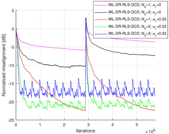
Figure 4.
Misalignment of the WL-DR-RLS-DCD algorithm for different values of and . The input signal is a speech sequence, and the length of the four unknown impulse responses is and . The four echo paths change in the middle of the simulation.
6. Discussion
The proposed WL-DR-RLS-DCD algorithm has several advantages compared to previous work. First, as compared to the DR-RLS method presented in [23], the proposed solution has two specific features: (i) it can be applied in the framework of SAEC thanks to the WL model, as shown in Section 2, and (ii) it achieves a lower computational complexity due to the DCD iterations, as presented in Section 3 and Section 4. Second, as compared with the WL-RLS-DCD from [5], the proposed version leads to better tracking capabilities due to the DR approach, as also supported by the simulation results presented in Section 5.
As mentioned in Section 4 and Section 5, the WL-DR-RLS-DCD algorithm also comes with some compromises. When increasing the number of DR iterations (i.e., the value of ), the algorithm runs the DCD iterations for a number of times. The arithmetic complexity needed for solving the associated auxiliary systems of equations becomes proportional to the parameter (besides the length of the complex valued adaptive filter and ). However, in practice, the values of and , are small, and the overall costs associated with the WL-DR-RLS-DCD, in terms of necessary chip areas, remain attractive for practical implementations on hardware devices.
Another part of the compromise corresponding to the DR approach is the loss of some accuracy at steady state for the WL-DR-RLS-DCD with respect to the WL-RLS-DCD. In order to mitigate this downside, we can employ several adjustments to the WL-DR-RLS-DCD, which add minimal extra arithmetic costs. Based on past experience with implementation of variable parameters for adaptive algorithms, a new version of the WL-DR-RLS-DCD with a variable number of DR iterations for SAEC scenarios can be developed. The new algorithm will adjust the value of with respect to the convergence state of the algorithm by gradually increasing it when approaching steady state and by decreasing it when tracking situations occur.
Furthermore, we will explore the option of mitigating the DR accuracy reduction at steady state by employing a variable forgetting factor approach, which was studied by our team in [26,27]. The goal is to implement a system with variable memory features in order to counteract the negative aspects of the compromise between convergence speed and accuracy.
A third option is to apply decomposition techniques based on the nearest Kronecker product (NKP), in conjunction with the DR version [28,29,30]. The DR-NKP approach applied on the WL-RLS-DCD would replace a single long adaptive filter with a combination of two shorter filters. Consequently, the advantage of such decomposition is twofold. Gains can be obtained in terms of both performance and complexity.
7. Conclusions
The paper proposed a low-complexity RLS algorithm for SAEC scenarios with enhanced tracking capabilities. The new WL-DR-RLS-DCD is derived from the already established WL-RLS-DCD method, and it employs an acceptable arithmetic workload in order to adapt faster to changes in the environment. The information presented in Table 1 and Table 3, respectively, shows that the overall arithmetic complexity remains proportional to the length of the complex valued filter multiplied by a small value, making the WL-DR-RLS-DCD an attractive choice for hardware implementations. Furthermore, simulation results demonstrated that the DR approach can improve the tracking performance of the RLS-DCD-type algorithms when working with highly correlated input signals, such as AR sequences and speech.
The simulations also revealed that increasing the number of DR iterations (i.e., the value of ) leads to a reduction in accuracy at steady state. Consequently, as explained in Section 6, our future efforts will be concentrated on developing low-complexity versions of the RLS algorithm for SAEC scenarios based on the DCD method, with variable parameters, such as the number of DR iterations or the forgetting factor . Moreover, we will invest research effort into applying decomposition techniques of impulse responses by exploiting associated low-rank approximations.
Author Contributions
Conceptualization, C.-L.S., C.P. and J.B.; formal analysis, C.-L.S., C.P. and J.B.; methodology, C.-L.S. and I.-D.F.; software, I.-D.F. and C.-L.S. All authors have read and agreed to the published version of the manuscript.
Funding
This work was supported by two grants of the Ministry of Research, Innovation and Digitization, CNCS–UEFISCDI, projects PN-III-P1-1.1-TE-2021-0393 and PN-III-P4-PCE-2021-0438, within PNCDI III.
Institutional Review Board Statement
Not applicable.
Informed Consent Statement
Not applicable.
Data Availability Statement
The data presented in this study are available on request from the corresponding author.
Conflicts of Interest
The authors declare no conflict of interest.
References
- Haykin, S. Adaptive Filter Theory; Prentice-Hall Information and System Sciences Series; Prentice Hall: Upper Saddle River, NJ, USA, 2002. [Google Scholar]
- Sayed, A. Adaptive Filters; Wiley: New York, NY, USA, 2008. [Google Scholar]
- Diniz, P.S.R. Adaptive Filtering: Algorithms and Practical Implementation, 4th ed.; Springer: New York, NY, USA, 2013. [Google Scholar]
- Benesty, J.; Paleologu, C.; Gaensler, T.; Ciochina, S. A Perspective on Stereophonic Acoustic Echo Cancellation; Springer: Berlin/Heidelberg, Germany, 2011; Volume 4. [Google Scholar] [CrossRef]
- Stanciu, C.; Benesty, J.; Paleologu, C.; Gänsler, T.; Ciochină, S. A widely linear model for stereophonic acoustic echo cancellation. Signal Process. 2013, 93, 511–516. [Google Scholar] [CrossRef]
- Hänsler, E.; Schmidt, G. Acoustic Echo and Noise Control–A Practical Approach; Wiley: Hoboken, NJ, USA, 2004. [Google Scholar]
- Enzner, G.; Buchner, H.; Favrot, A.; Kuech, F. Acoustic echo control. In Academic Press Library in Signal Processing; Elsevier: Amsterdam, The Netherlands, 2014; Volume 4, pp. 807–877. [Google Scholar] [CrossRef]
- Sondhi, M.; Morgan, D.; Hall, J. Stereophonic acoustic echo cancellation-an overview of the fundamental problem. IEEE Signal Process. Lett. 1995, 2, 148–151. [Google Scholar] [CrossRef]
- Benesty, J.; Morgan, D.; Sondhi, M. A better understanding and an improved solution to the specific problems of stereophonic acoustic echo cancellation. IEEE Trans. Speech Audio Process. 1998, 6, 156–165. [Google Scholar] [CrossRef]
- Malik, S.; Wung, J.; Atkins, J.; Naik, D. Double-Talk Robust Multichannel Acoustic Echo Cancellation Using Least-Squares MIMO Adaptive Filtering: Transversal, Array, and Lattice Forms. IEEE Trans. Signal Process. 2020, 68, 4887–4902. [Google Scholar] [CrossRef]
- Hong, J. Stereophonic Acoustic Echo Suppression for Speech Interfaces for Intelligent TV Applications. IEEE Trans. Consum. Electron. 2018, 64, 153–161. [Google Scholar] [CrossRef]
- Cho, B.J.; Park, H.M. Stereo Acoustic Echo Cancellation Based on Maximum Likelihood Estimation with Inter-Channel-Correlated Echo Compensation. IEEE Trans. Signal Process. 2020, 68, 5188–5203. [Google Scholar] [CrossRef]
- Zhang, H.; Wang, D. Neural Cascade Architecture for Multi-Channel Acoustic Echo Suppression. IEEE/ACM Trans. Audio Speech Lang. Process. 2022, 30, 2326–2336. [Google Scholar] [CrossRef]
- Romoli, L.; Cecchi, S.; Peretti, P.; Piazza, F. A Mixed Decorrelation Approach for Stereo Acoustic Echo Cancellation Based on the Estimation of the Fundamental Frequency. IEEE Trans. Audio Speech Lang. Process. 2012, 20, 690–698. [Google Scholar] [CrossRef]
- Schneider, M.; Huemmer, C.; Kellermann, W. Wave-domain loudspeaker signal decorrelation for system identification in multichannel audio reproduction scenarios. In Proceedings of the 2013 IEEE International Conference on Acoustics, Speech and Signal Processing, Vancouver, BC, USA, 26–31 May 2013; pp. 605–609. [Google Scholar] [CrossRef]
- Romoli, L.; Cecchi, S.; Piazza, F. A novel decorrelation approach for multichannel system identification. In Proceedings of the 2014 IEEE International Conference on Acoustics, Speech and Signal Processing (ICASSP), Florence, Italy, 4–9 May 2014; pp. 6652–6656. [Google Scholar] [CrossRef]
- Schneider, M.; Kellermann, W. Multichannel Acoustic Echo Cancellation in the Wave Domain With Increased Robustness to Nonuniqueness. IEEE/ACM Trans. Audio Speech Lang. Process. 2016, 24, 518–529. [Google Scholar] [CrossRef]
- Stanciu, C.; Benesty, J.; Paleologu, C.; Gaensler, T.; Ciochină, S. A novel perspective on stereophonic acoustic echo cancellation. In Proceedings of the IEEE International Conference on Acoustics, Speech and Signal Processing (ICASSP), Kyoto, Japan, 25–30 March 2012; pp. 25–28. [Google Scholar] [CrossRef]
- Stanciu, C.; Paleologu, C.; Benesty, J.; Gaensler, T.; Ciochina, S. An efficient RLS algorithm for stereophonic acoustic echo cancellation with the widely linear model. In Proceedings of the 41st International Congress and Exposition on Noise Control Engineering, INTERNOISE, New York, NY, USA, 19–22 August 2012; Volume 9, pp. 7756–7767. [Google Scholar]
- Breining, C.; Dreiscitel, P.; Hansler, E.; Mader, A.; Nitsch, B.; Puder, H.; Schertler, T.; Schmidt, G.; Tilp, J. Acoustic echo control. an application of very-high-order adaptive filters. IEEE Signal Process. Mag. 1999, 16, 42–69. [Google Scholar] [CrossRef]
- Zakharov, Y.V.; White, G.P.; Liu, J. Low-Complexity RLS Algorithms Using Dichotomous Coordinate Descent Iterations. IEEE Trans. Signal Process. 2008, 56, 3150–3161. [Google Scholar] [CrossRef]
- Zakharov, Y.V.; Nascimento, V.H. DCD-RLS Adaptive Filters with Penalties for Sparse Identification. IEEE Trans. Signal Process. 2013, 61, 3198–3213. [Google Scholar] [CrossRef]
- Paleologu, C.; Benesty, J.; Ciochină, S. Data-Reuse Recursive Least-Squares Algorithms. IEEE Signal Process. Lett. 2022, 29, 752–756. [Google Scholar] [CrossRef]
- Fîciu, I.D.; Stanciu, C.L.; Elisei-Iliescu, C.; Anghel, C.; Udrea, R.M. Low-Complexity Implementation of a Data-Reuse RLS Algorithm. In Proceedings of the 2022 45th International Conference on Telecommunications and Signal Processing (TSP), Virtual, 13–15 July 2022; pp. 289–293. [Google Scholar] [CrossRef]
- The Open Speech Repository. Available online: https://www.itu.int/rec/T-REC-G.168/en (accessed on 5 November 2022).
- Paleologu, C.; Benesty, J.; Ciochina, S. A Robust Variable Forgetting Factor Recursive Least-Squares Algorithm for System Identification. IEEE Signal Process. Lett. 2008, 15, 597–600. [Google Scholar] [CrossRef]
- Stanciu, C.; Paleologu, C.; Benesty, J.; Ciochina, S.; Albu, F. Variable-forgetting factor RLS for stereophonic acoustic echo cancellation with widely linear model. In Proceedings of the 2012 Proceedings of the 20th European Signal Processing Conference (EUSIPCO), Bucharest, Romania, 27–31 August 2012; pp. 1960–1964. [Google Scholar]
- Paleologu, C.; Benesty, J.; Ciochină, S. Linear System Identification Based on a Kronecker Product Decomposition. IEEE/ACM Trans. Audio Speech Lang. Process. 2018, 26, 1793–1808. [Google Scholar] [CrossRef]
- Elisei-Iliescu, C.; Paleologu, C.; Benesty, J.; Stanciu, C.; Anghel, C.; Ciochină, S. Recursive Least-Squares Algorithms for the Identification of Low-Rank Systems. IEEE/ACM Trans. Audio Speech Lang. Process. 2019, 27, 903–918. [Google Scholar] [CrossRef]
- Dogariu, L.M.; Benesty, J.; Paleologu, C.; Ciochină, S. Identification of Room Acoustic Impulse Responses via Kronecker Product Decompositions. IEEE/ACM Trans. Audio Speech Lang. Process. 2022, 30, 2828–2841. [Google Scholar] [CrossRef]
Disclaimer/Publisher’s Note: The statements, opinions and data contained in all publications are solely those of the individual author(s) and contributor(s) and not of MDPI and/or the editor(s). MDPI and/or the editor(s) disclaim responsibility for any injury to people or property resulting from any ideas, methods, instructions or products referred to in the content. |
© 2023 by the authors. Licensee MDPI, Basel, Switzerland. This article is an open access article distributed under the terms and conditions of the Creative Commons Attribution (CC BY) license (https://creativecommons.org/licenses/by/4.0/).