Article

Support Vector Machine (SVM) Application for Uniaxial Compression Strength (UCS) Prediction: A Case Study for Maragheh Limestone

1
School of Information Engineering, Yancheng Teachers University, Yancheng 224002, China
2
Faculty of Technology, Sivas Cumhuriyet University, Sivas 58140, Turkey
3
Department of Civil Engineering, University of Tabriz, Tabriz 5166616471, Iran
4
Department of Earth Sciences, Utrecht University, 3584 CB Utrecht, The Netherlands
*
Author to whom correspondence should be addressed.
Appl. Sci. 2023, 13(4), 2217; https://doi.org/10.3390/app13042217
Submission received: 29 November 2022 / Revised: 8 January 2023 / Accepted: 30 January 2023 / Published: 9 February 2023
(This article belongs to the Special Issue Predictive Modeling in Mining and Geotechnical Engineering)

Abstract

:

Featured Application

AI application in UCS prediction for limestones of Maragheh.

Abstract

The geomechanical properties of rock materials, such as uniaxial compression strength (UCS), are the main requirements for geo-engineering design and construction. A proper understanding of UCS has a significant impression on the safe design of different foundations on rocks. So, applying fast and reliable approaches to predict UCS based on limited data can be an efficient alternative to regular traditional fitting curves. In order to improve the prediction accuracy of UCS, the presented study attempted to utilize the support vector machine (SVM) algorithm. Multiple training and testing datasets were prepared for the UCS predictions based on a total of 120 samples recorded on limestone from the Maragheh region, northwest Iran, which were used to achieve a high precision rate for UCS prediction. The models were validated using a confusion matrix, loss functions, and error tables (MAE, MSE, and RMSE). In addition, 24 samples were tested (20% of the primary dataset) and used for the model justifications. Referring to the results of the study, the SVM (accuracy = 0.91/precision = 0.86) showed good agreement with the actual data, and the estimated coefficient of determination (R2) reached 0.967, showing that the model’s performance was impressively better than that of traditional fitting curves.

1. Introduction

The geomechanical properties of rock masses involve the intact rock features and discontinuity networks [1]. The intact rock features represent valuable information about a rock’s stiffness and strength parameters, which are considered to be the principal geotechnical design index requirements [2,3]. These index parameters, such as uniaxial compression strength (UCS), cohesion (c), angle of internal friction (φ), elastic modulus (E), shear modulus (G), bulk modulus (K), and P-wave modulus (M), are measured by direct and indirect geotechnical laboratory tests, which are performed on obtained samples, recovered cores, and on-site specimens under specific instructions. Direct methods involve experimental measurements applied to the rock material in the laboratory or on site. To perform these experiments, the special instructions, devices, and methods that are used have been standardized by international or national organizations [4]. The UCS (also known as the unconfined compressive strength) test is the first experiment applied on rock samples to estimate the maximum strength of the intact rock against axial loading [5], which is the maximum axial compressive stress that a right-cylindrical sample of material can withstand before failure [6]. UCS represents the compressive strength of a rock, which can be defined as the ability of the rock to resist forces imposed on it or the maximum stress that a sample can withstand under specified loading conditions.
On the other hand, UCS directly informs geo-engineers about a rock’s durability and its ultimate strength under different loading stages, providing essential data in the design stages to avoid structural failure and instabilities. This makes the UCS measurement very important in geo-engineering practice. ASTM D7012 [7] provides a description of the experimental procedure for the testing of samples.
Estimating a rock’s geomechanical index properties such as its UCS guarantees the success of design and construction assurance. So, accurate measurements are key points in evaluations. Traditional methods dictate that to achieve the appropriate level of accuracy, the number of samples should be high and repeatable (regarding the scope, sensitivity, and scale of the project) so that the average values can be calculated with less error. A low volume of samples will increase uncertainties and errors in the measurements. Using a large number of samples for a UCS test requires a long time period and is very costly. Thus, applying alternative methods that require a shorter period with less financial leverage that reaches a good accuracy is always welcomed. With the advances in computer-based algorithms, the geo-material strength indexes for different materials can be predicted and can achieve the expected level of reliability. Subsequently, many scientific researchers have launched various aspects of related research related to these predictions [8]. These studies have been implemented to complete the advancements of traditional procedures to estimate the geomechanical index properties of rock materials based on UCS, point-load [9], or Schmidt hammer [10] results.
Recently, predictive techniques have changed significantly after the introduction of machine learning to geotechnical applications, especially material behavior predictions [11,12,13,14]. Singh et al. [15] and Sonmez et al. [16] provided artificial neural network (ANN)-based predictive models for predicting several sedimentary and igneous intact rock index behaviors. Yılmaz and Yuksek [17,18] applied multilayer perceptron (MLP) as one of the most-common ANN-based predictive models to estimate geo-mechanical features indexes such as UCS based on UCS and point-load (Is) test results conducted on gypsum samples from Sivas in Turkey. Kahraman et al. [19] applied the same technique (MLP) to predict the UCS values from samples taken from Misis Fault Breccia in Nigde, Turkey. The results were used for a deformability evaluation in the studied site. Dehghan et al. [20], Bahrami et al. [21], and Yurdakul et al. [22] applied several types of machine learning classifiers to evaluate and predict UCS variations compared to regression models, which indicated that the predictive model showed a good performance in estimating the indices. The coefficient of determination (R2) is the main criterion used to estimate predictive performances. Armaghani et al. [23] and Armaghani et al. [24] applied MLP, support vector machine (SVM), and other benchmark algorithms to predict the UCS values of shale and granite samples utilized for predicting geomechanical index behavioral evaluations. Mozumder and Laskar [25] used the same neural network to identify the UCS changes in compacted clayey soils as stiff materials. Their results were incredibly close to the actual data during the prediction process. Abdi et al. [26] developed a forecasting model to obtain the relationship between UCS and the elastic modulus (E) in sedimentary rocks, which was appropriately used to estimate the correlation for different types of sediment units by using regular regression analysis. Barham et al. [12] used the coupled MLP with ordinary multivariate regression analysis to implement a predictive model for masonry samples taken from Jordan to predict the UCS variations in the materials.
Using computational techniques such as machine learning improves the reliability of predictive models with reasonable accuracy and low errors, according to the literature cited. Regarding these claims, regression analysis is used to establish a correlation between the UCS values from the predictive model and the measured data and the prediction models created by the machine learning classifiers. This link can further enhance the prediction accuracy of forecasting the UCS of samples. To this end, the presented study attempted to use one of the most-efficient benchmark machine learning algorithms, SVM, to analyze and predict UCS variations in sedimentary rocks from the Maragheh region in Iran. SVM-based models are supervised learning models with associated algorithms for classification and regression analysis. The SVM method works relatively well when there is a clear margin of separation between classes. It is more effective in high-dimensional spaces and cases where the dimensions are greater than the number of samples. In addition, SVM is relatively memory efficient and is widely used in classifications related to forecasting procedures [27]. The presented study used these advantages to prepare a predictive model for analysis and predict UCS variations in Maragheh limestone, which was mainly implemented in a Python high-level programming environment [28].
The main objective of this article was to provide a reliable model to classify and predict the UCS values for limestone-type sedimentary rocks from the Maragheh region. Given that the traditional and usual methods of conducting extensive tests and using experimental regression methods to determine the changes in the resistance of rock masses are costly and time-consuming, methods that effectively reduce the cost and increase the speed of analysis have recently gained the attention of rock engineering experts. In this regard, computer models and artificial intelligence can be used to estimate the resistance parameters of rock masses, especially UCS. As an achievement, this is of interest to geo-engineers. So, the presented study attempted to use an SVM-supervised model to classify and predict the UCS of rock samples from the studied region.

2. Materials and Methods

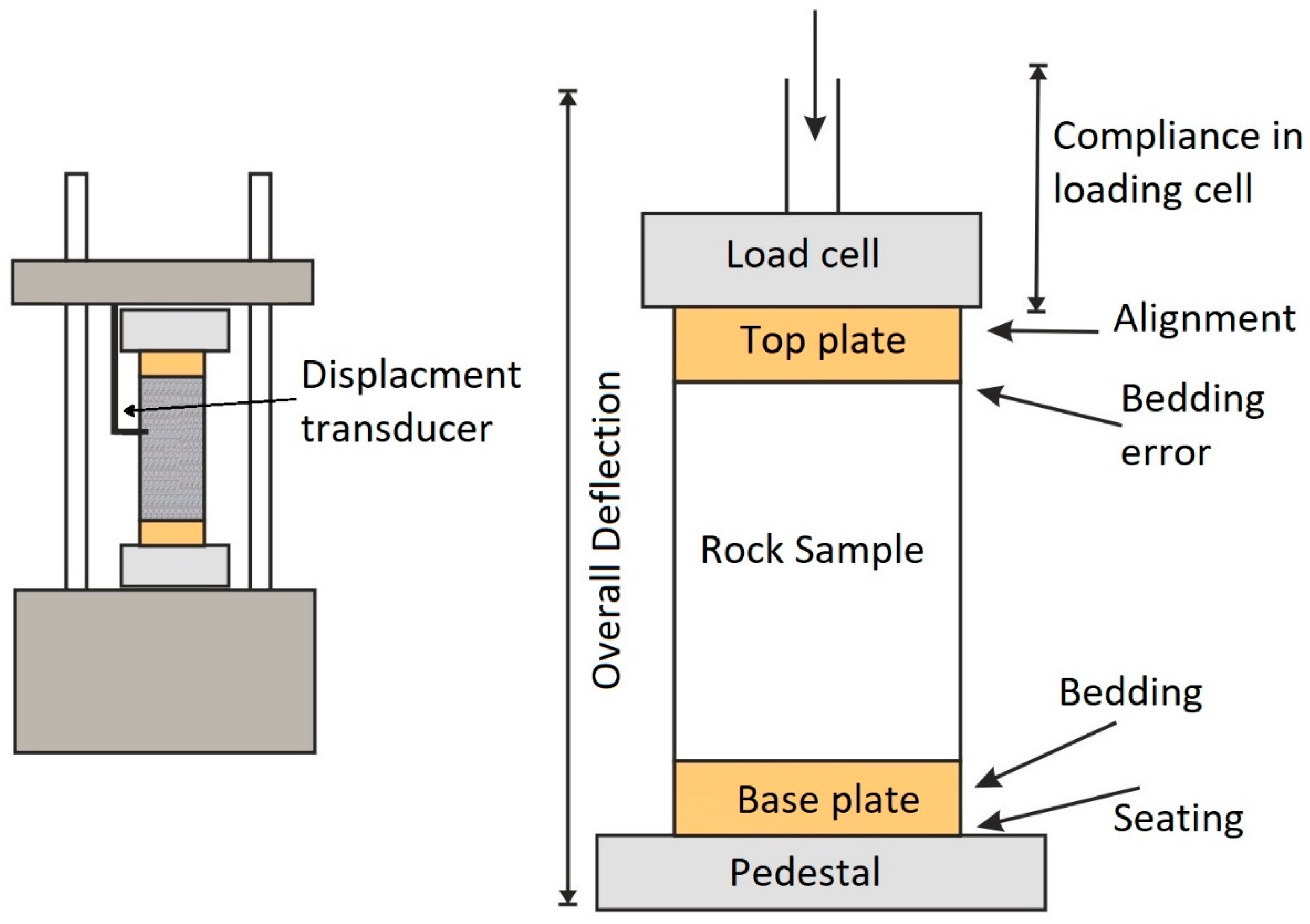
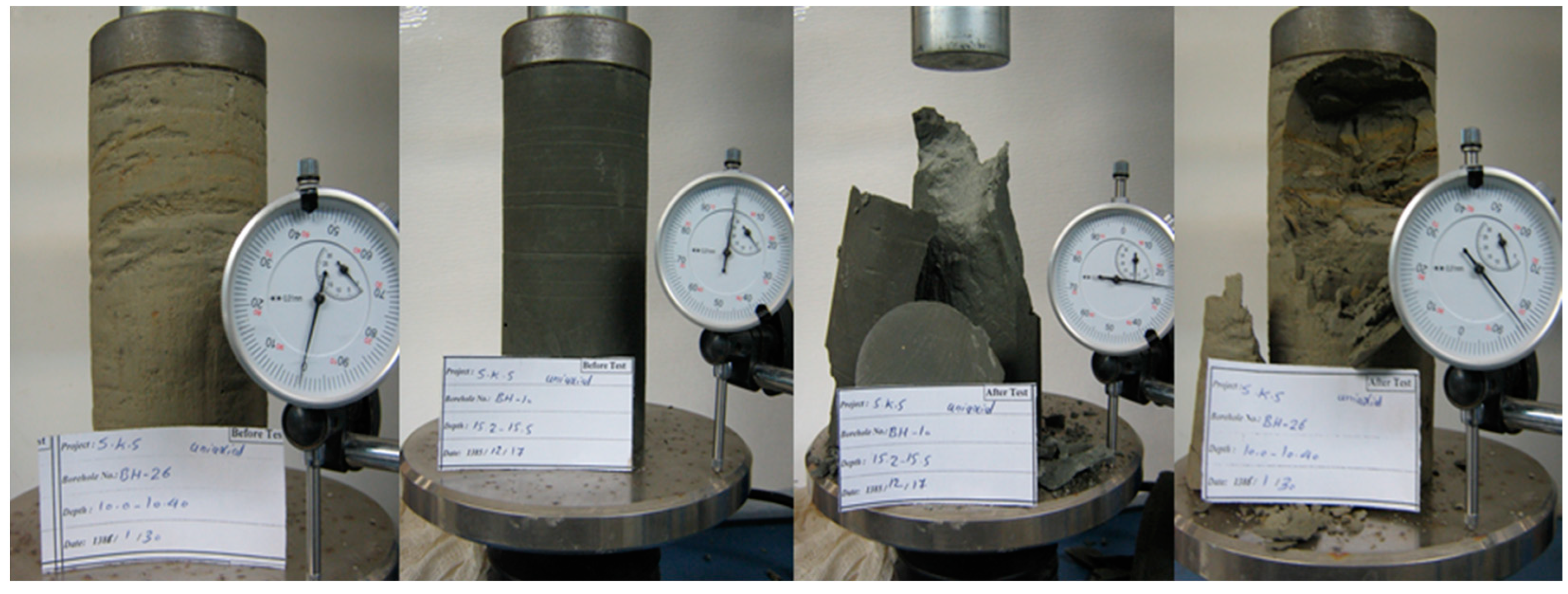
2.1. Laboratory Studies

Uniaxial compression strength, or UCS, is the standardized universal test that can be performed on all types of rock specimens that is used by the American Society for Testing and Materials, ASTM [7], and the International Society for Rock Mechanics, ISRM [29]. The principle of UCS involves placing cylindrical samples or prepared drill cores under axial loading until the failure moment in a uniaxial compression test (UCT) device. Figure 1 illustrates a conventional rock UCT machine [30]. The UCT is used for the determination of the ultimate UCS values. The presented study used regular cylindrical specimens for testing via the UCT in a geotechnical laboratory. The rock samples in this study were obtained from limestone from Maragheh County, located in East Azerbaijan province, northwest Iran. In total, 120 samples were taken from the studied region, where the main component of the rock is calcium carbonate and is categorized as Argillaceous lime to limestone with a 75% to 100% carbonate content according to the Pettijohn classification [31]. After sampling the limestone from the site, the specimens were prepared according to the ASTM instructions and tested via the UCT [7]. In order to prepare the test specimens, the taken samples were transferred into the geotechnical laboratory and drilled with a 50 mm diameter (5 cm) and a 100 mm height (10 cm) with an overall cylindrical shape. These specimens were cut and polished to produce UCS samples with smooth and flat surfaces and no evident fissures, as per the ASTM requirements. After preparation, all samples were divided and tested regarding the UCS compression test, and the results were recorded. During the tests, the water content of the samples was natural, and the tests were conducted at room temperature. The results of these tests were prepared and inputted into the primary database for implementing the SVM-based predictive modeling.
Figure 2 illustrates several limestone images in the laboratory during the UCS test, which was used for preparing the SVM primary dataset. According to the ASTM [7] instructions, providing a proper sample is one of the key steps in UCS testing, as this leads to a reduction in measurement errors. UCS tests are typically performed on intact rocks with standard lengths of 100 mm (prepared) or with NQ, HQ, or PQ diamond drill cores, and the maximum axial loading is recorded at the failure point [1]. The correct preparation of samples leads to the obtaining of more reliable UCS values and classified accuracy of a rocks’ strength. The International Society for Rock Mechanics (ISRM) standard classification for UCS variation in rock is very low (<5 MPa), low (5–25 MPa), moderate (25–50 MPa), medium (50–100 MPa), high (100–250 MPa), and very high (250< MPa) [32]. Sedimentary rock is generally classified as being in the very low to medium classes [11]. Nevertheless, the UCS corresponds to axial loading, where peak stress is responsible for the failure of a rock sample. Using displacement transducers and strain gages, the stress–strain data were continuously logged and recorded.

2.2. Artificial-Intelligence-Based Modeling

2.2.1. SVM Algorithm Principles

Support vector machine or SVM is a set of supervised learning methods used for classification, regression, and outlier detection. SVM was initially developed by Cortes and Vapnik in AT&T Bell Laboratories [33] and was operated based on statistical learning frameworks, namely the Vapnik–Chervonenkis theory [34], and can be applied in both linear and non-linear classifications. The linear SVM uses a maximum-margin hyperplane (hard-margin or soft-margin), and the non-linear SVM utilizes kernels for classifications. SVM is also used for unsupervised learning, which is called support vector clustering (SVC) [27]. SVM algorithms use differing types of kernel functions, whose most-common functions are linear, nonlinear, polynomial, radial basis function, and sigmoid [31]. The present study used a sigmoid kernel function. This kernel function is similar to a two-layer perceptron model of a neural network, which works as an activation function for neurons. So, using such a function helps to modify the prediction process similarly to neural networks. SVM classifies the input data during the training by using a maximum-margin hyperplane derived by solving the optimization. There are specialized algorithms for quickly solving the quadratic programming (QP) problem that arises from SVM that generally rely on heuristics to break the problem down into smaller, more manageable chunks. Another approach is to use an interior-point method that uses Newton-like iterations to find a solution to the Karush–Kuhn–Tucker conditions of primal and dual problems [35]. Instead of solving a sequence of broken-down issues, this approach directly solves the problem altogether.
To avoid solving a linear system involving a large kernel matrix, a low-rank approximation to the matrix is often used in the kernel trick [27]. Drucker et al. [36] proposed a version of SVM for regression and prediction called support-vector regression (SVR), which is a model produced by support-vector classification that depends only on a subset of the training data because the loss function for building the model does not care about training points that lie beyond the margin. Analogously, the model produced by SVR depends only on a subset of the training data because the loss function for building the model ignores any training data close to the model prediction [37,38]. Training the original SVR involves solving the following equations [38]:
minimize   w 2 2 + C i = 1 N ( ξ i + ξ i * ) subject   to | y i < w , x i > b | ε
where w is the vector normal to the hyperplane (margin), C is a quadratic function, b is the width from the origin, ξi is the slack variable, C is the width from the hyperplane, xi is a training sample with a target value (yi), ε is a free parameter, and i = {1,2,3,…., N}. The inner product plus the intercept <w,xi> −b is the prediction for that sample, and ε is a free parameter that serves as a threshold; all predictions have to be within an ε range of the true predictions. Slack variables are usually added into the above to allow for errors and to allow an approximation in case the above problem is infeasible. There is a target value for different values of ε, which has an impact on the regression analysis and prediction results. The present study used an SVM-supervised classifier for the prediction and regression evaluation for the UCS prediction for a prepared dataset of Maragheh limestone.

2.2.2. Data Analysis and Inspection

In this study, 120 specimens were taken from different spatial locations in the Maragheh Region located in East Azerbaijan province, northwest Iran. The sampling distribution from the studied area was specifically selected so that samples represented Maragheh limestone. The samples were prepared and tested via ASTM instructions [7], and the results were recorded during the experimental stage. These data were used to prepare the main database of the predictive and verification models. The database was randomly divided into testing and training sets. The testing set contained 20% of the primary database, and the training set included 70% of the main database. The SVM model was trained with a training set and validated with a testing set. The training set contained 96 samples, and the testing set contained 24 samples of data. The coefficient of determination (R2) was used to establish correlations between the predicted and measured data during the experimental as well as the prediction stages.

2.2.3. Model Implementation

The SVM models were used to predict the compressive strength of the Maragheh limestone based on the gathered comprehensive database of the 120 concluded UCS testing results that were divided into the testing and training datasets. The confusion matrix and loss function estimated the model trained with a training set and tested it with a testing set regarding the accuracy, model performance, and capability. The confusion matrix is a performance evaluator used for machine learning classifiers with evaluation criteria that include accuracy, precision, recall, and the harmonic mean [28,38,39]. The results of this table represent the performance and capability of the predictive model in terms of its accurate prediction and perfect operation. In this table, the criteria vary from 0 to 1, with 0 being the lowest and 1 being the highest. The loss function (or cost function) is a function that maps an event or values of variables onto an actual number, intuitively representing some ‘loss’ associated with the event. The loss function provides information about the mathematical optimization and seeks to minimize errors regarding the prediction and measured values. So, it is a difference between the estimated and valid values for a data instance [27]. The loss function helps to understand the capacity of the predictive model for both the training and testing sets to learn appropriately. This function was used in this task to demonstrate the learning rate for the SVM model. The models learned under specific optimizing functions that improved the learning rates. The learning rate is a configurable hyperparameter used in training procedures for machine learning algorithms. Table 1 provides information about the utilized hyperparameters in the different applied classifiers.

2.2.4. Model Validation and Justification

Of course, the confusion matrix and loss function represent the predictive model’s validation during the learning stages, but for controlling the model’s performance, we used a statistical errors table that included the mean absolute error (MAE), mean square error (MSE), and root mean square error (RMSE). These error tables are frequently used to measure the differences between the predicted values generated by a model and the measured values obtained by tests [40]. Generally, a lower number of computational errors indicates a better algorithm performance [28].

3. Results and Discussion

3.1. Laboratory Studies

After the testing stage, according to the standard procedure, all the UCS values were measured and categorized. Statistical analysis is one of the most important stages for providing appropriate ground data. Although various indexes for multi-indicator analysis for geomaterials [41,42,43] exist, in SVM modeling, the predictive analysis is usually based on two directions and two variables. Therefore, underrating the target values is much more important. The main uncertainty [44] regarding the model in this study belonged to the UCS values, which could be modified by considering the distribution function and normalized by the Q–Q chart, as presented in Figure 3 and Figure 4. Table 2 provides the statistical variations in the estimated UCS values for the Maragheh limestone. The quantile–quantile chart (known as the Q–Q chart) was obtained for the UCS results to examine the normality of the data variations, as illustrated in Figure 3. Based on the results of the statistical analysis of the UCS data, it was indicated that the average UCS value measured for the studied limestone was 109.93 MPa, and the calculated standard deviation was 39.754. Regarding the Q–Q chart, the experimental data followed a normal distribution law within the confidence interval of 93.7%. This fact was verified using a normal distribution envelope on the UCS data, as shown in Figure 4.

3.2. Artificial-Intelligence-Based Modeling

The SVM algorithm was implemented on the training and testing datasets to predict the UCS variation for the studied limestone. Figure 5 provides the predicted values of the UCS values from the SVM model against the measured values, which were correlated by using R2, representing the dependency of the measured and predicted variables. R2 is the link between the actual outcomes and the predicted values that normally range from 0 to 1, where if it is closer to 1, a higher accuracy of the data overlap appears. According to Figure 5, the estimated R2 for the UCS results was 0.967, which was considerable for a shallow learning classifier. In addition, Figure 6 provides information about the overlap of the actual and predicted values of the UCS. As seen in this figure, there were good agreements between the actual and predicted data. In addition, the loss rate calculated for the model was reduced to 0.2 in the training set. So, the model was appropriately implemented and operated with a high performance and could predict the UCS with less error. Table 3 illustrates the errors table estimated for the SVM model regarding the prediction process. Based on Table 3, it was indicated that the training set operated with fewer errors than the testing set; the error rates for the training set were MAE = 0.237463, MSE = 0.210540, and RMSE = 0.200674, where these rates for the testing set were 0.451089, 0.435988, and 0.410456, respectively. Figure 7a provides the scatter index error for the UCS results. Figure 7b provides the Willmott index for the error variations for the UCS results.
Figure 8 presents the decision boundary and probability for the scattering data with SVM, which was used to categorize the data during the learning and testing procedures. As seen in this figure, the accuracy of the boundary and probability indexes reached 0.7, which showed the model’s high performance. The model was validated using a confusion matrix (evaluation criteria included accuracy, precision, and recall), the loss function, and an errors table. The results of the validated learning classifier are provided in Figure 9 and Figure 10. Figure 9 shows the confusion matrix of the predictive model, and Figure 7 presents the calculated loss function. According to Figure 9, the model’s estimated accuracy, precision, and recall were 0.91, 0.86, and 0.80, respectively. Figure 10 provides information about the loss function variations for the testing and training datasets, which was reduced to 0.2. This value indicated a considerable reduction in the error rate during the learning procedure. Figure 11 provides the statistical analysis index conducted on the results of the SVM modeling on the training and testing datasets. In addition, the predicted results of the used model, along with the corresponding measured values in both the testing and training datasets as well as the prediction errors, are presented in Figure 12.
The application of the SVM algorithm is appropriate for different types of geo-material behavioral predictions, and researchers in future scientific projects can consider this. However, it should be noted that the SVM algorithm is unsuitable for large datasets and when facing datasets with noise. So, users must be notified when they attempt to utilize the SVM or SVP models in the prediction process. In addition, if a probabilistic analysis needs to be conducted, SVM classifiers are not capable of using a probabilistic explanation for the classification. Although these limitations are general aspects of SVM and provide sufficient coverage and accuracy for the analyses of intact rocks, they have to be considered in analyses such as when analyzing the anisotropy of rocks.

4. Conclusions

The presented study attempted to apply an SVM-supervised classifier to classify and predict the compressive strength (UCS) behavior of Maragheh limestone. In this regard, a comprehensive field survey and sampling were performed in the Maragheh region, leading to a total of 120 specimens of limestone being obtained from different sites in the studied region. The samples were isolated and transferred into a geotechnical laboratory to conduct UCS tests as per ASTM regulations in a UCT device. After performing the laboratory and modeling procedures, the following results were obtained:
  • An extensive database was provided using the UCS experimental records to provide a detailed analysis of the SVM model. The prepared database was randomly divided into a training test (80% of the primary database) and a testing set (the remaining 20% of the primary database). The SVM model was trained on the training set and tested on the testing dataset.
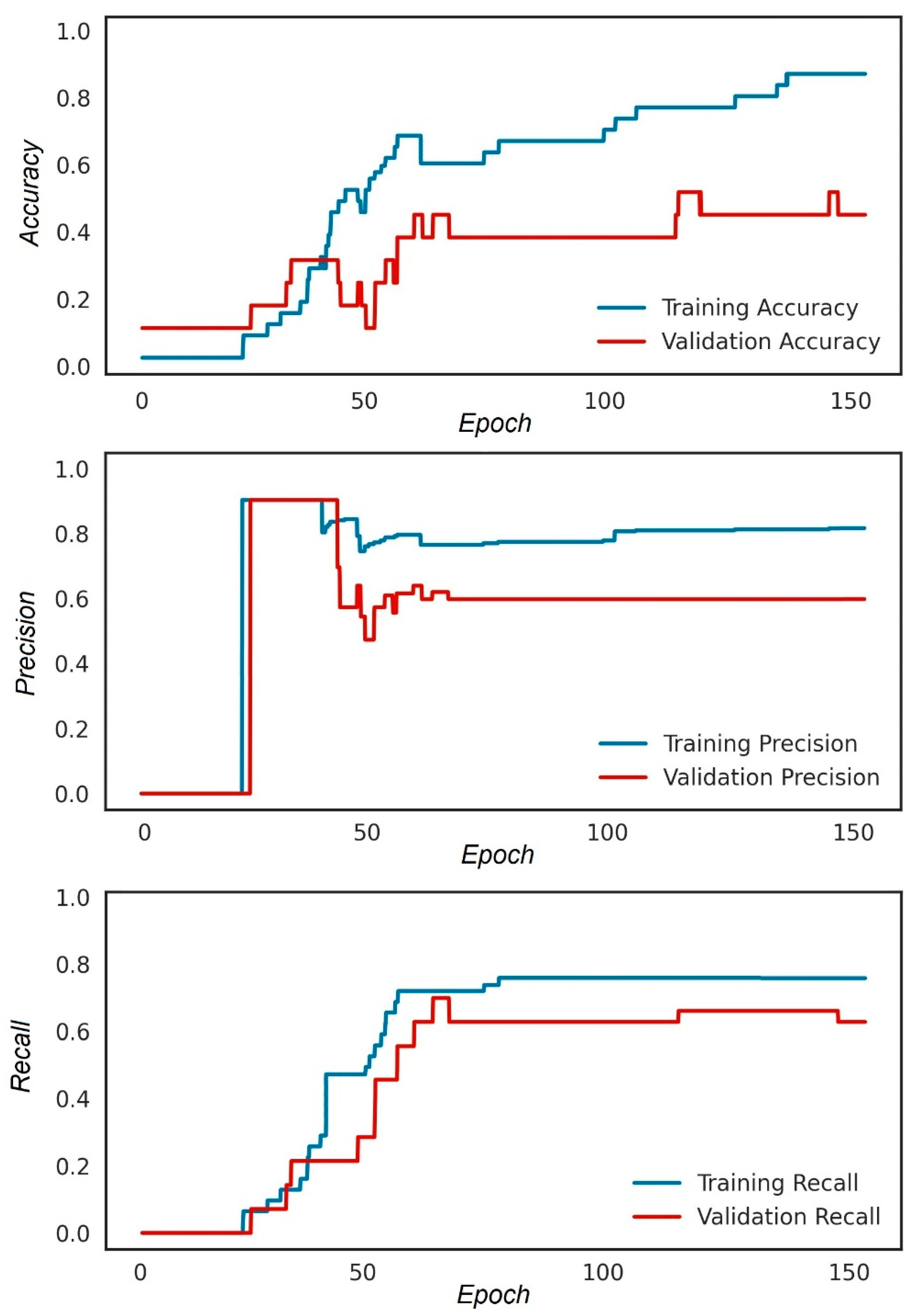
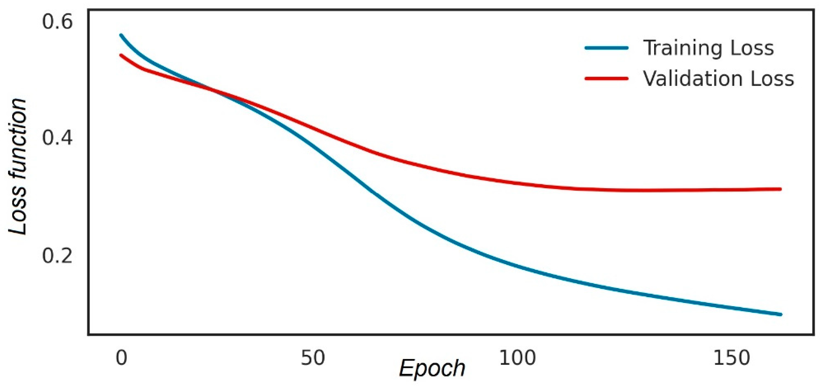
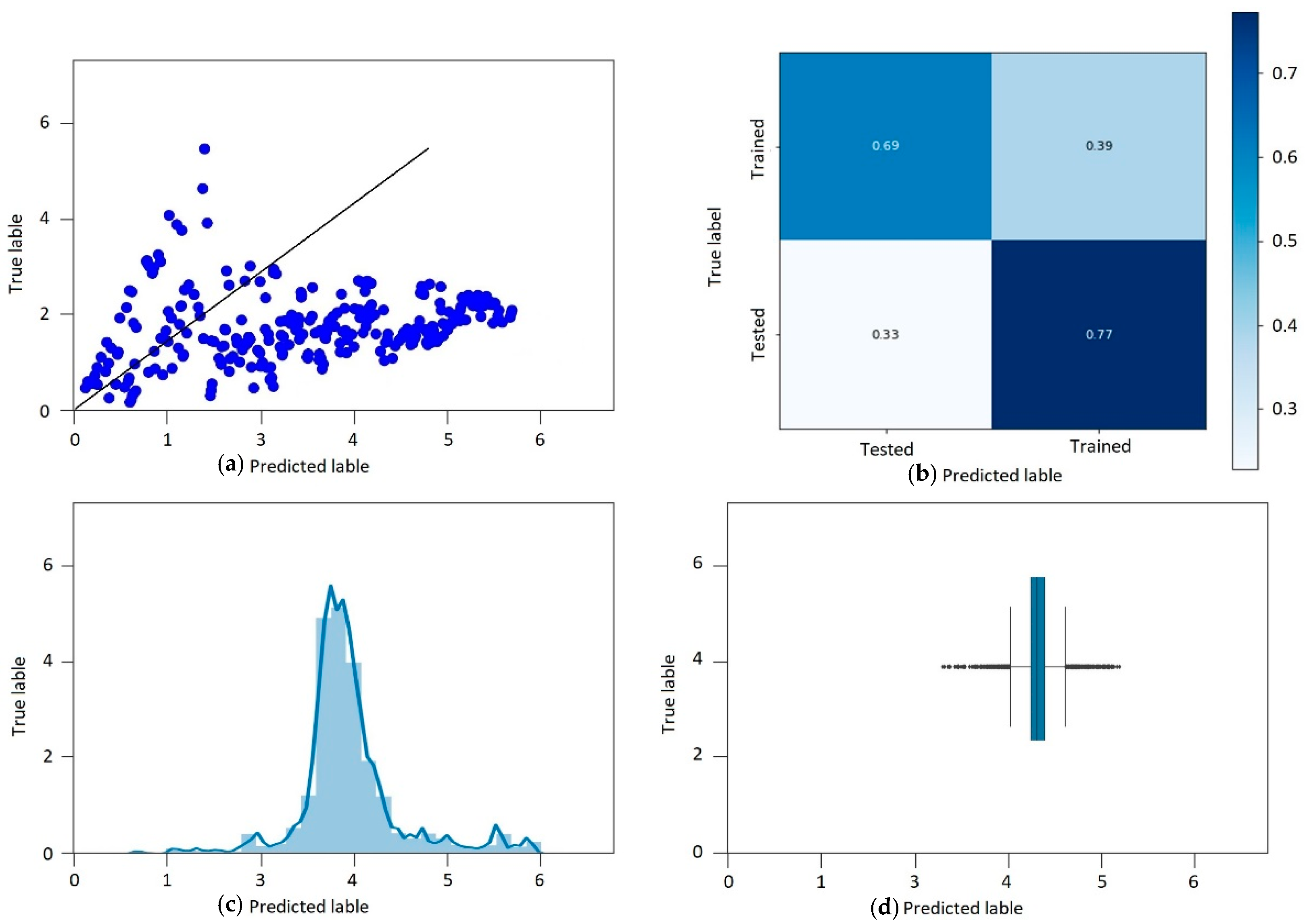
  • The machine learning technique was controlled by a confusion matrix, loss function, and statistical error analysis for both the testing and training datasets, which provided relevant information about the capability and performance of the model.
  • According to the SVM results, the model’s accuracy was 0.91, and its precision was 0.86. In addition, the estimated loss function was reduced to 0.2, which is considered to be a good capability for learning. In addition, the other evaluating criteria, such as recall, were estimated at about 0.78, which is considerable for the learning rate of the SVM model.
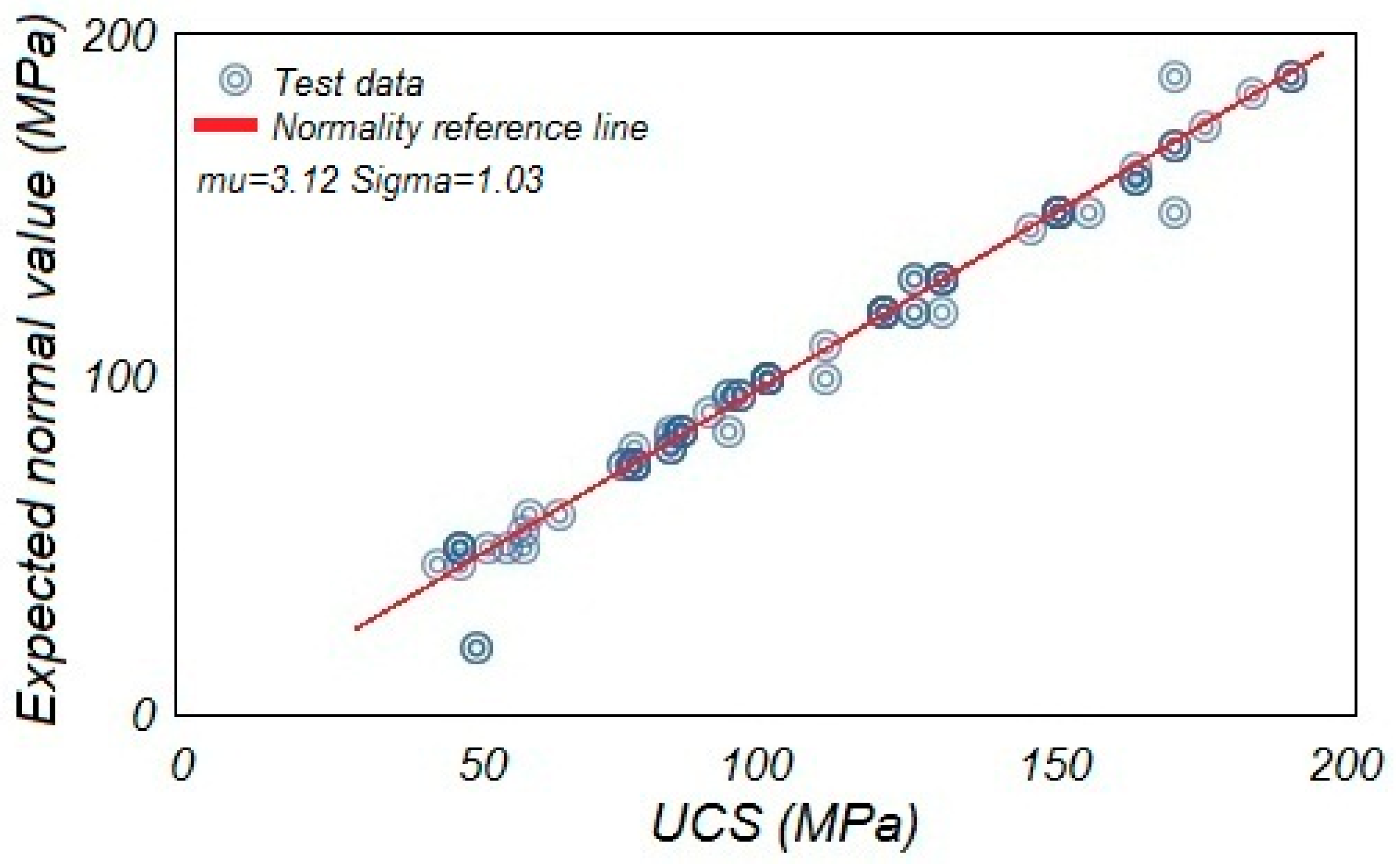
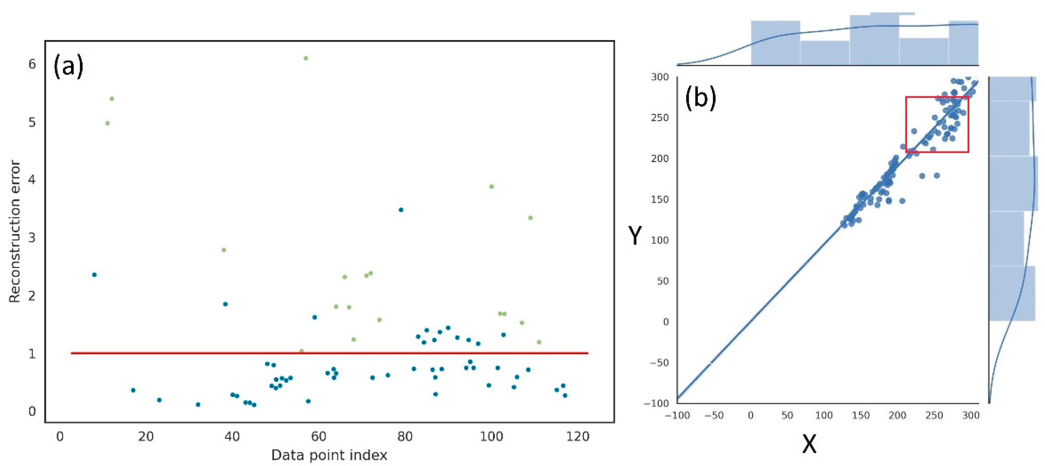
  • By normalizing the experiment data with the Q–Q chart, it appeared that the data chart followed a normal distribution law within the confidence interval of 93.7%.
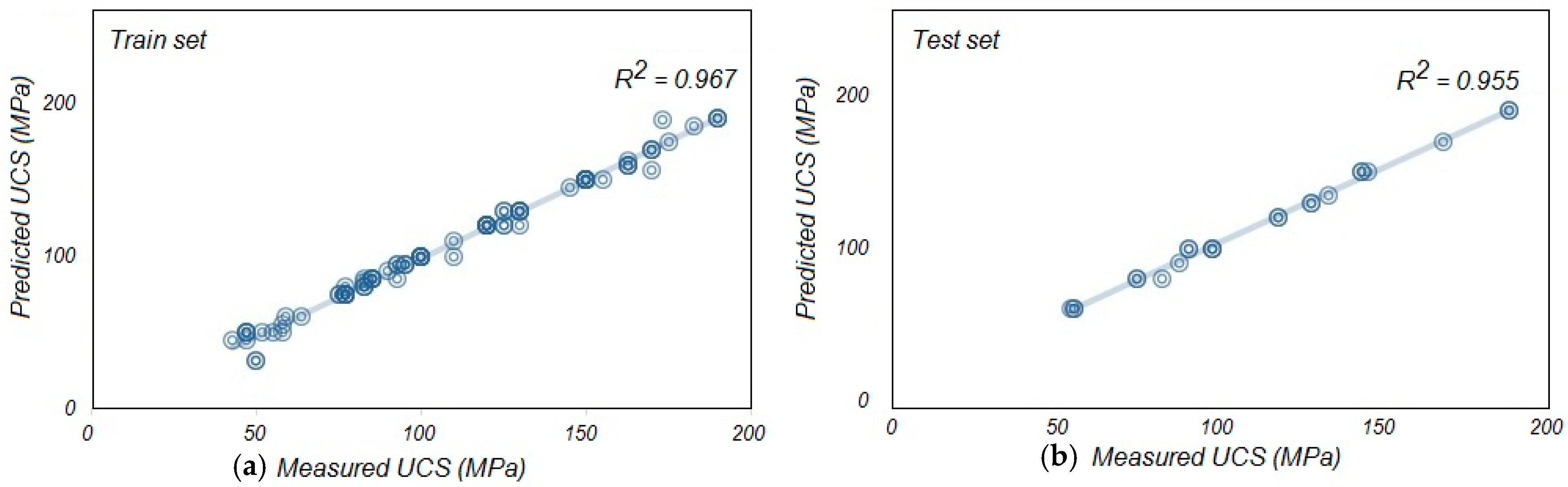
  • The correlation results for both the testing and training data with the actual results from the experiments indicated that the model was trained remarkably well (R2 = 0.967) and was tested properly (R2 = 0.955).
The statistical error rates obtained for the SVM model indicated that the model operated with a low error rate, including MAE = 0.237463, MSE = 0.210540, and RMSE = 0.200674 for the training set and 0.451089, 0.435988, and 0.410456 for the testing set, respectively.

Author Contributions

A.C., L.Z. and S.A.: writing—original draft preparation, validation, methodology, investigation, resources; J.X. and X.Y.: visualization, methodology; M.A. and R.D.: supervision, formal analysis, conceptualization, writing—review and editing. All authors have read and agreed to the published version of the manuscript.

Funding

This research received no external funding.

Institutional Review Board Statement

Not applicable.

Informed Consent Statement

Not applicable.

Data Availability Statement

Not applicable.

Acknowledgments

The authors wish to thank the Department of Civil Engineering, University of Tabriz, for providing permission to conduct the geotechnical investigations. In addition, the authors would like to thank the anonymous reviewers for providing invaluable review comments and recommendations for improving the scientific level of the article.

Conflicts of Interest

The authors declare no conflict of interest.

Abbreviations

UCSUniaxial compression strength
SVMSupport vector machine
SVRSupport vector regression
SVCSupport vector clustering
MLPMultilayer perceptron
QPQuadratic programming
MAEMean absolute error
R2Coefficient of determination
MSEMean square error
RMSERoot mean square error
Q–Q chartQuantile–quantile chart
Std.Dev.Standard deviation
UCTUniaxial compression test device
cCohesion
φInternal friction
EElastic modulus
GShear modulus
KBulk modulus
MP-wave modulus

References

  1. Harrison, J.P.; Hudson, J.A. Engineering Rock Mechanics: Illustrative Worked Examples; Elsevier Science: Amsterdam, The Netherlands, 2000. [Google Scholar]
  2. Jaeger, J.; Cook, N.G.; Zimmerman, R. Fundamentals of Rock Mechanics; Wiley-Blackwell: Oxford, UK, 2007. [Google Scholar]
  3. Mogi, K. Experimental Rock Mechanics; T&F Books; CRC Press: London, UK, 2009. [Google Scholar]
  4. Feng, X.T. Rock Mechanics and Engineering. In Volume 2: Laboratory and Field Testing; CRC Press: Boca Raton, FL, USA, 2017. [Google Scholar]
  5. Azarafza, M.; Ghazifard, A.; Akgun, H.; Asghari-Kaljahi, E. Geotechnical characteristics and empirical geo-engineering rela-tions of the South Pars Zone marls, Iran. Geomech. Eng. 2019, 19, 393–405. [Google Scholar] [CrossRef]
  6. Azarafza, M.; Akgün, H.; Asghari-Kaljahi, E. Assessment of rock slope stability by slope mass rating (SMR): A case study for the gas flare site in Assalouyeh, South of Iran. Geomech. Eng. 2017, 13, 571–584. [Google Scholar] [CrossRef]
  7. ASTM D7012; Standard Test Methods for Compressive Strength and Elastic Moduli of Intact Rock Core Specimens under Varying States of Stress and Temperatures. ASTM International: West Conshohocken, PA, USA, 2014.
  8. Li, S.; Wang, Y.; Xie, X. Prediction of Uniaxial Compression Strength of Limestone Based on the Point Load Strength and SVM Model. Minerals 2021, 11, 1387. [Google Scholar] [CrossRef]
  9. Kohno, M.; Maeda, H. Relationship between point load strength index and uniaxial compressive strength of hydrothermally altered soft rocks. Int. J. Rock Mech. Min. Sci. 2012, 50, 147–157. [Google Scholar]
  10. Azarafza, M.; Ghazifard, A.; Asasi, F.; Rahnamarad, J. An empirical classification method for South Pars marls by Schmidt hammer rebound index. MethodsX 2021, 8, 101366. [Google Scholar] [CrossRef]
  11. Heidari, M.; Mohseni, H.; Jalali, S.H. Prediction of uniaxial compressive strength of some sedimentary rocks by fuzzy and regression models. Geotech. Geol. Eng. 2018, 36, 401–412. [Google Scholar] [CrossRef]
  12. Barham, W.S.; Rabab’ah, S.R.; Aldeeky, H.H.; AL Hattamleh, O.H. Mechanical and physical based artificial neural network models for the prediction of the unconfined compressive strength of rock. Geotech. Geol. Eng. 2020, 38, 4779–4792. [Google Scholar] [CrossRef]
  13. Raja, M.N.A.; Shukla, S.K. Predicting the settlement of geosynthetic-reinforced soil foundations using evolutionary artificial intelligence technique. Geotext. Geomembr. 2021, 49, 1280–1293. [Google Scholar] [CrossRef]
  14. Kardani, N.; Aminpour, M.; Raja, M.N.A.; Kumar, G.; Bardhan, A.; Nazem, M. Prediction of the resilient modulus of compacted subgrade soils using ensemble machine learning methods. Transp. Geotech. 2022, 36, 100827. [Google Scholar] [CrossRef]
  15. Singh, V.K.; Singh, D.; Singh, T.N. Prediction of strength properties of some schistose rocks from petrographic properties using artificial neural networks. Int. J. Rock Mech. Min. Sci. 2001, 38, 269–284. [Google Scholar] [CrossRef]
  16. Sonmez, H.; Gokceoglu, C.; Nefeslioglu, H.A.; Kayabasi, A. Estimation of rock modulus: For intact rocks with an artificial neural network and for rock masses with a new empirical equation. Int. J. Rock Mech. Min. Sci. 2006, 43, 224–235. [Google Scholar] [CrossRef]
  17. Yılmaz, I.; Yuksek, A.G. An Example of artificial neural network (ANN) application for indirect estimation of rock parameters. Rock Mech. Rock Eng. 2008, 41, 781–795. [Google Scholar] [CrossRef]
  18. Yılmaz, I.; Yuksek, A.G. Prediction of the strength and elasticity modulus of gypsum using multiple regression, ANN and ANFIS models. Int. J. Rock Mech. Min. Sci. 2009, 46, 803–810. [Google Scholar] [CrossRef]
  19. Kahraman, S.; Gunaydin, O.; Alber, M.; Fener, M. Evaluating the strength and deformability properties of Misis fault breccia using artificial neural networks. Exp. Syst. Appl. 2009, 36, 6874–6878. [Google Scholar] [CrossRef]
  20. Dehghan, S.; Sattari, G.H.; Chehre-Chelgani, S.; Aliabadi, M.A. Prediction of uniaxial compressive and modulus of elasticity for travertine sample using regression and artificial neural networks. Int. J. Min. Sci. Technol. 2010, 20, 41–46. [Google Scholar] [CrossRef]
  21. Bahrami, A.; Monjezi, M.; Goshtasbi, K.; Ghazvinian, A. Prediction of rock fragmentation due to blasting using artificial neural network. Eng. Comput. 2011, 27, 177–181. [Google Scholar] [CrossRef]
  22. Yurdakul, M.; Ceylan, H.; Akdas, H. A predictive model for uniaxial compressive strength of carbonate rocks from Schmidt hardness. In Proceedings of the 45th US Rock Mechanics/Geomechanics Symposium, San Francisco, CA, USA, 26–29 June 2011; pp. 511–533. [Google Scholar]
  23. Armaghani, D.J.; Hajihassani, M.; Bejarbaneh, B.Y.; Marto, A.; Mohamad, E.T. Indirect measure of shale shear strength pa-rameters by means of rock index tests through an optimized artificial neural network. Measurement 2015, 55, 487–498. [Google Scholar] [CrossRef]
  24. Armaghani, D.J.; Mohamad, E.T.; Momeni, E.; Monjezi, M.; Narayanasamy, M.S. Prediction of the strength and elasticity modulus of granite through an expert artificial neural network. Arab. J. Geosci. 2016, 9, 48. [Google Scholar] [CrossRef]
  25. Mozumder, R.A.; Laskar, A.I. Prediction of unconfined compressive strength of geopolymer stabilized clayey soil using Artificial Neural Network. Comput. Geotech. 2015, 69, 291–300. [Google Scholar]
  26. Abdi, Y.; Taheri Garavand, A.; Zarei Sahamieh, A. Prediction of strength parameters of sedimentary rocks using artificial neural networks and regression analysis. Arab. J. Geosci. 2018, 11, 587. [Google Scholar] [CrossRef]
  27. Cristianini, N.; Shawe-Taylor, J. An Introduction to Support Vector Machines and Other Kernel-Based Learning Methods; Cambridge University Press: Cambridge, UK, 2000. [Google Scholar]
  28. Müller, A.C.; Guido, S. Introduction to Machine Learning with Python: A Guide for Data Scientists; O’Reilly Media: Sebastopol, CA, USA, 2016. [Google Scholar]
  29. Bieniawski, Z.T. Suggested Method on Uniaxial Compressive Strength and Deformability of Rock Materials. Int. J. Rock Mech. Min. Sci. Geomech. Abstr. 1979, 16, 137–140. [Google Scholar] [CrossRef]
  30. Isah, B.W.; Mohamad, H.; Ahmad, N.R.; Harahap, I.S.H.; Al-bared, M.A.M. Uniaxial compression test of rocks: Review of strain measuring instruments. IOP Conf. Ser. Earth Environ. Sci. 2020, 476, 012039. [Google Scholar] [CrossRef]
  31. Pettijohn, F.J. Sedimentary Rock, 3rd ed.; Harpercollins: New York, NY, USA, 1983. [Google Scholar]
  32. Ulusay, R. The ISRM Suggested Methods for Rock Characterization, Testing and Monitoring; Springer: New York, NY, USA, 2016. [Google Scholar]
  33. Cortes, C.; Vapnik, V.N. Support-vector networks. Mach. Learn. 1995, 20, 273–297. [Google Scholar] [CrossRef]
  34. Vapnik, V.N. Statistical Learning Theory; Wiley-Interscience: New York, NY, USA, 1989. [Google Scholar]
  35. Ferris, M.C.; Munson, T.S. Interior-Point Methods for Massive Support Vector Machines. SIAM J. Optim. 2002, 13, 783–804. [Google Scholar] [CrossRef]
  36. Drucker, H.; Burges, C.C.; Kaufman, L.; Smola, A.J.; Vapnik, V.N. Support Vector Regression Machines. In Advances in Neural Information Processing Systems; NIPS 1996; ACM Digital Library: New York, NY, USA, 1997; Volume 9, pp. 155–161. [Google Scholar]
  37. Awad, M.; Khanna, R. Support vector regression. In Efficient Learning Machines; Apress: Berkeley, CA, USA, 2015. [Google Scholar]
  38. Zhang, F.; O’Donnell, L.J. Support Vector Regression; Academic Press: New York, NY, USA, 2020. [Google Scholar]
  39. Khan, M.U.A.; Shukla, S.K.; Raja, M.N.A. Soil–Conduit interaction: An artificial intelligence application for reinforced concrete and corrugated steel conduits. Neural Comput. Appl. 2021, 33, 14861–14885. [Google Scholar]
  40. Azarafza, M.; Azarafza, M.; Akgün, H.; Atkinson, P.M.; Derakhshani, R. Deep learning-based landslide susceptibility mapping. Sci. Rep. 2021, 11, 1–16. [Google Scholar]
  41. Raja, M.N.A.; Shukla, S.K. Multivariate adaptive regression splines model for reinforced soil foundations. Geosynth. Int. 2021, 28, 368–390. [Google Scholar]
  42. Benemaran, R.S.; Esmaeili-Falak, M.; Javadi, A. Predicting resilient modulus of flexible pavement foundation using extreme gradient boosting based optimised models. Int. J. Pavement Eng. 2022, 1–20. [Google Scholar] [CrossRef]
  43. Khan, N.M.; Cao, K.; Yuan, Q.; Hashim, M.H.B.M.; Rehman, H.; Hussain, S.; Khan, S. Application of Machine Learning and Multivariate Statistics to Predict Uniaxial Compressive Strength and Static Young’s Modulus Using Physical Properties under Different Thermal Conditions. Sustainability 2022, 14, 9901. [Google Scholar] [CrossRef]
  44. Zhao, G.; Wang, H.; Li, Z. Capillary water absorption values estimation of building stones by ensembled and hybrid SVR models. J. Intell. Fuzzy Syst. 2022, 44, 1–13. [Google Scholar] [CrossRef]
Figure 1. Regular UCT testing device [30].
Applsci 13 02217 g001
Figure 2. An image of the limestone samples and UCS test device used in this study.
Applsci 13 02217 g002
Figure 3. The Q–Q chart for normality tests of UCS results.
Applsci 13 02217 g003
Figure 4. The normal distribution envelope of UCS results.
Applsci 13 02217 g004
Figure 5. Correlation between the actual and predicted UCS results: (a) training set, (b) testing set.
Applsci 13 02217 g005
Figure 6. Overlap between the actual and predicted UCS results: (a) training set, (b) testing set.
Applsci 13 02217 g006
Figure 7. (a) Scattered and (b) Willmott’s index for error variations for UCS results.
Applsci 13 02217 g007
Figure 8. Demonstration of index values for the case of overprediction.
Applsci 13 02217 g008
Figure 9. The evaluation criteria estimated for SVM model.
Applsci 13 02217 g009
Figure 10. The estimated loss function for the SVM model.
Applsci 13 02217 g010
Figure 11. Statistical specifications of the SVM model’s results: (a) Pearson’s correlation coefficient, (b) heat map, (c) frequency distribution, and (d) boxplot diagram.
Applsci 13 02217 g011
Figure 12. The corresponding (a) predicted and measured values and (b) prediction error variations.
Applsci 13 02217 g012
Table 1. The hyperparameters used in utilized models.
ClassifierHyperparametersElements
SVMKernels
C value
Kernel = ‘sigmoid’; Degree = 2
C = 100; Epsilon = 0.1
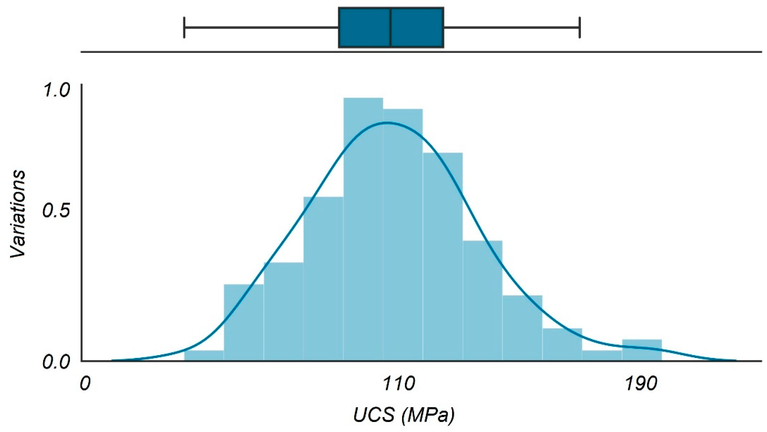
Table 2. Statistical analysis for Maragheh limestone UCS results.
ParameterMaxMinMeanStd.Dev.VarianceSkewness
UCS19043109.9339.754158.0440.214
Max = maximum value, Min = minimum value, and Std.Dev. = standard deviation.
Table 3. Comparison of SVM model performance for Maragheh limestone UCS results.
Analysis SetMAEScoreMSEScoreRMSEScoreR2ScoreA10-IndexScoreRank
Training0.2374620.2105420.2006720.96720.9317210
Testing0.4510810.4359810.4104510.95510.914815
Disclaimer/Publisher’s Note: The statements, opinions and data contained in all publications are solely those of the individual author(s) and contributor(s) and not of MDPI and/or the editor(s). MDPI and/or the editor(s) disclaim responsibility for any injury to people or property resulting from any ideas, methods, instructions or products referred to in the content.

