Three-Dimensional Geological Modeling of the Shallow Subsurface and Its Application: A Case Study in Tongzhou District, Beijing, China

Abstract

Three-dimensional (3D) geological models are currently needed and used independently for urban development. The main difficulty in constructing a 3D geological model of a shallow subsurface is to determine the stratigraphic distribution. Highly variable properties and geometries of geological units beneath lead to difficulty. It is key to find a practicable and efficient way to construct a model in practical work. This study takes Tongzhou District (Beijing) as a case; 476 boreholes (40 newly drilled and 436 existing engineering boreholes) were utilized combined with the cross-section method to construct an integrated 3D geological model. The framework and analyses contributed to the following applications: (1) High-quality information from new boreholes and existing engineering boreholes were used to define stratigraphy and build cross-sections. (2) The resulting geological model (up to 50 m beneath Tongzhou area) shows many details of the shallow subsurface. This includes 10 major layers which were grouped into three cyclothems representing cyclic sequences of clay, interbedded silt, sand, and gravel with variable quantities of lenses. (3) The new model was used as a tool to visualize the depth and geometry variations below ground and to characterize a large variety of properties (for example, the compression modulus analyzed in this paper) that each unit contains, and then to evaluate the underground geological conditions. (4) An analysis of a dynamic monitoring model based on the resulting 3D model indicated that the geological units (sand and silty clay) at depths between 30 m and 40 m, with an average vertical deformation of 0.97 mm, from July 2019 to September 2020, are suitable for underground construction, from the perspective of vertical stability in the study area. Monitoring models that take time into consideration based on a 3D framework will be further explored.

1. Introduction

The rapid development of urban underground space (UUS) requires a solid understanding of the subsurface, especially shallow subsurface conditions. As a solid space composed of gas, water, soils, and rocks, the underground is completely within the geological environment [1]. Hence, the complexity and variability of geological conditions are vital reasons for uncertainty and potential risks during future UUS construction. Research on geological conditions of the urban shallow subsurface has been systematically developed during the last 20 years [2,3,4,5,6]. However, delineating the stratigraphic structures of the subsurface in detail in an urban setting is still challenging, because the properties of shallow geological layers upon which urban infrastructure and municipal utilities are built are heterogeneous [7,8]. Although the geological and geotechnical investigation method provides detailed information at discrete locations [8], soil properties can be highly variable in the vertical direction. Three-dimensional (3D) geological modeling is then developed as an effective method to describe such variability subsoils exhibit in both horizontal and vertical directions. In an urban setting, it is challenging to construct a 3D geological model.

As an effective tool to visualize the urban subsurface [9,10,11,12], 3D geological modeling has been developing quickly in the past decades [8,13,14,15,16,17,18,19,20]. This method can deliver a better understanding of the subsurface structures [21,22,23,24,25,26] and portray the properties that are heterogeneously distributed within geological bodies [17,27,28,29].

Additionally, a variety of 3D geological models has been constructed to aid resource evaluation [6,9], to explore geological conditions [30,31,32,33], and to study the geotechnical properties of the subsoils [7,10,34,35] to promote understanding of shallow subsurfaces. Researchers from the British Geological Survey [2,5,12,36,37] have constructed a variety of 3D geological models at all scales from sites to cities to the UK landmass and continental shelf using various software tools and modelling approaches [38]; Hou et al. [9] built a 3D geological model to establish the UUS quality level and distribution in Foshan city in Guangdong Province, China; Ye et al. [33] constructed a 3D model of land subsidence to simulate groundwater flow aquifer system displacements in downtown Shanghai (China); Høyer et al. [39] developed a high-resolution 3D geological model of Samsø (Denmark) to update the risk assessment of the Pillemark landfill; Anderson et al. [3] constructed an integrated 3D geological model of Vejle, Denmark, to support urban planning by providing planning maps; and Chen et al. [40] presented an integrated MPS-based 3D model framework in Minjiang Estuary area (China) to achieve more precise visualization for the subsurface structures. In general, 3D geological models have increasingly been used to improve understanding of geology at different scales.

Three-dimensional geological models are currently needed and used independently of urban development; yet constructing a 3D geological model in an urban setting is still challenging considering the accessibility to data, data compilation, methods employed, and complex geological environments. Even though the use of different frameworks for modeling has been tested, few studies have presented systematic procedures and methods at a city scale in a complex alluvial fan sedimentary environment.

The main aim of this study is to develop an efficient and practical procedure of 3D geological modeling under a fluvial sedimentary environment in an urban area and discuss the applications. Taking Tongzhou District (Beijing) as a case, 40 new drilled boreholes combined with an existing 1506 files of investigation data were analyzed to support lithology generalization, a necessary step of the cross-section method. A detailed procedure of this method was discussed. Finally, a systematic modeling framework and an integrated 3D model (up to 50 m beneath Tongzhou) were constructed. The new model was used as a tool to visualize the depth and geometry variations below ground and to characterize a large variety of properties (for example, the compression modulus analyzed in this paper) that each unit contains and then to evaluate the underground geological conditions. Outputs combined with the thickness map of each geological unit revealed from the model can improve our understanding of geological conditions below ground and provide valuable insights to reduce construction risk in the future. The dynamic monitoring model that takes time into consideration is another key application, but more research is needed for dynamic models.

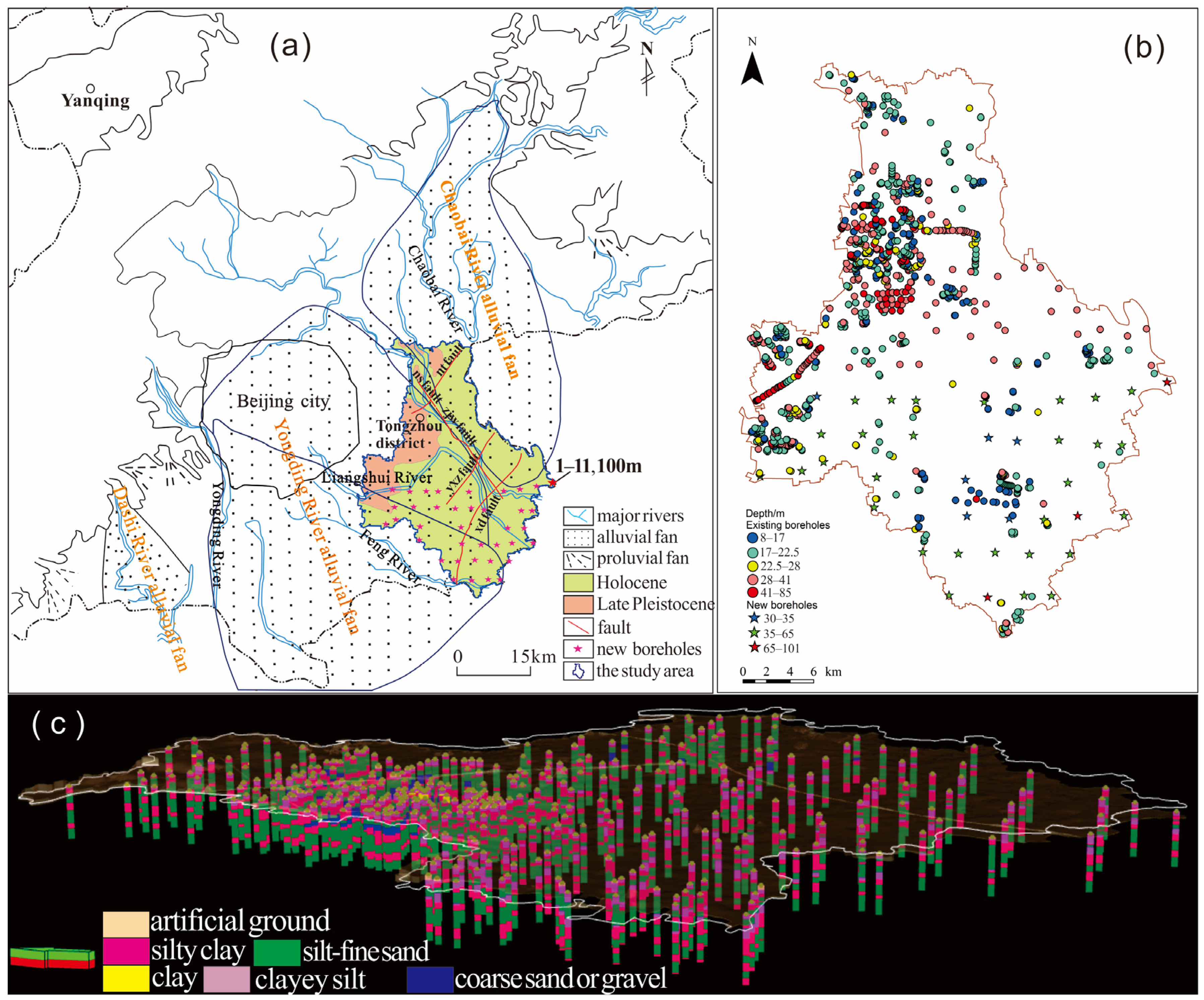
2. Quaternary Geology

The shallow subsurface deposits in the Beijing plain are composed of several huge alluvial fans and sedimentary depressions. Tongzhou District is located in the southeast of the Beijing plain, with the topography being slightly higher in the northwest and lower in the southeast. Three rivers, including the Wenyu River, Chaobai River, and Liangshui River, flow northwest and merge at the southeastern part of the study area (Figure 1). Quaternary deposits occur widely throughout the entire area and typically overlie the bedrock. Underlying the urban area, Holocene and Late Pleistocene sediments overlie Neogene sequences and Paleogene locally in the Southeast Depression. Tongzhou is the intersection zone of two large alluvial fans, i.e., the Yongding River and Chaobai River alluvial fans [41].

The earliest and largest one is the Yongding River alluvial fan, with the fan top located in Shijingshan District and spreading along the northwest–southeast direction, of which lithologies change from single gravel units in the west to multilayer structures of silty clay, clayey, sands, and gravel in the east [41]. The Chaobai River, the second largest river in Beijing, originates from Yanshan Mountain and flows southward to form the vast Chaobai River alluvial–proluvial fan (Figure 1). The continuous uplift of mountains and the intense decline of plains resulted in the presence of thick sediments. The maximum thickness of Quaternary sediments exceeds 450 m in the southern part [42]. This explains the highly variable sequences of deposits widely developed across the entire area.

3. Data and Method

3.1. Geological Data

A total of 1506 scanned files of investigation data recording borehole points and corresponding geotechnical reports was collected in the modeled area. In total, 614 files came from the Tongzhou District Urban Construction Archives, while the remaining 892 files were obtained from the Tongzhou District Architectural Survey and Design Institute. Most of these boreholes were shallow (30 m or less) and clustered around local construction sites in the north part of the study area, some having relatively poor lithological descriptions. To provide more information about the subsurface lithology and define the standard layer in the modeled area, 40 new deep boreholes (Figure 1a,b) (maximum depth 100 m, such as 1–11 on Figure 1a) were drilled in the south part of the Tongzhou area. In total, 476 boreholes (Figure 1c) with deeper depth (typically more than 30 m) and detailed descriptions were finally honored for modeling, containing information concerning position, borehole identifications, depth, elevation, coordinates, top, bottom, and lithology of layers.

We also included faults as an important factor in the modeling procedure. A total of five faults with upper breakpoints located in the shallow sediments (50 m or less) was considered, including Nankou-Sunhe fault, Nanyuan-Tongxian fault, Zhangjiawan fault, Xiadian fault, and Yaoxinzhuang fault [43,44,45]. Fault data were derived from the technical report of the project titled “Investigation of major geological problems in the sub-center of Tongzhou area”, which was implemented during 2016–2017 by the Beijing Institute of Geological Survey. However, few records document exact locations of upper breakpoints in shallow Quaternary sediments (<50 m); fault plane was hence modeled based on an average fault throw, which was around 1–2 m.

3.2. Method

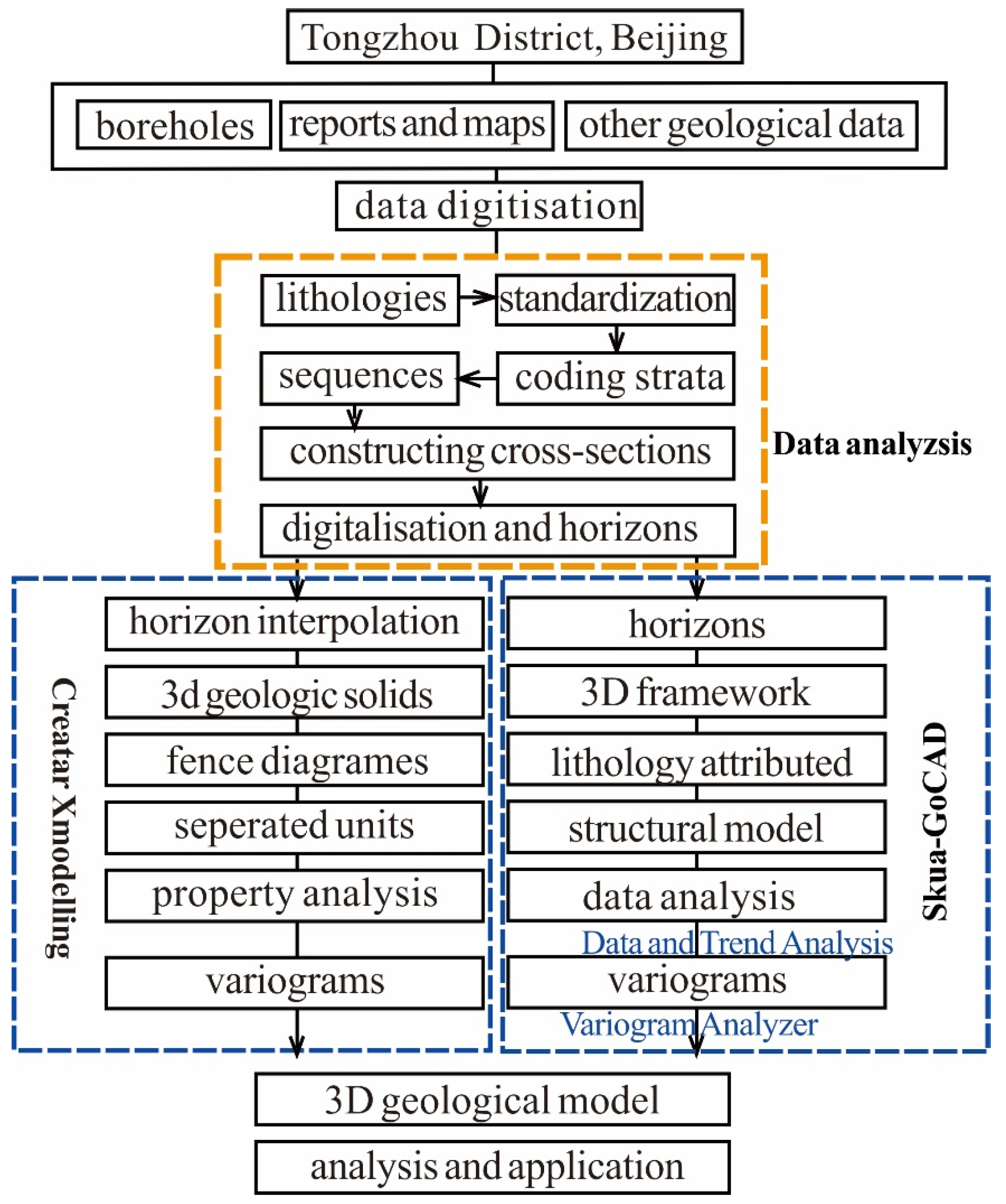
3.2.1. Three-Dimensional Modeling Workflow

In this work, both explicit and implicit methods were adopted to conduct the 3D geological model. Modeling was undertaken using both the SKUA-GoCAD software package, applied to implicit as well as explicit techniques (Structure and Stratigraphy and Reservoir Properties workflow), and Creatar Xmodelling for explicit modeling of Quaternary deposits in the shallow subsurface (Figure 2). The explicit modeling, for example, the cross-section method employed in this work (see Section 3.2.2), involves the interaction and implementation of geological concepts by geologists, while an implicit approach refers to the utilization of software programs embedded with mathematical functions based on geological concepts [38,46].

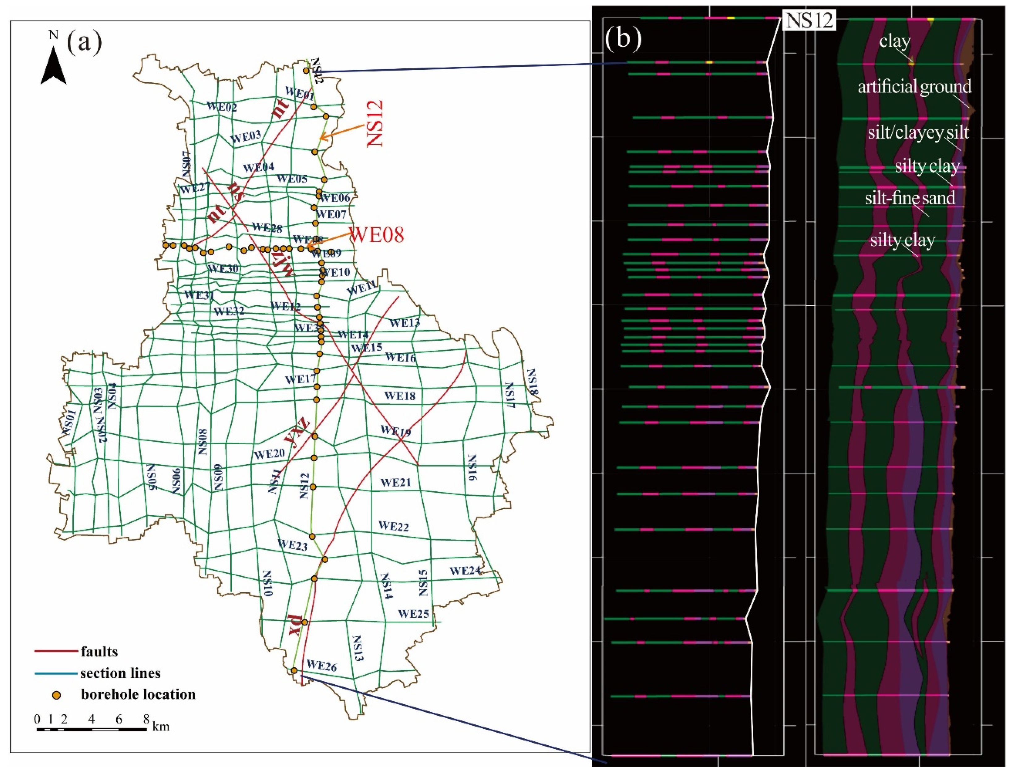
3.2.2. Cross-Section Method

A lack of universal standards across multiple data sources such as various engineering projects and the fact that soil types varied significantly from site to site (Figure 3) make data standardization difficult. This is compounded by the geological complexity modeled. Cross-sections are then constructed by selecting boreholes and combining lithology records with local geology to ensure consistency among unevenly distributed drill holes. This method comprises three major steps: (a) data digitalization, (b) lithology generalization, and (c) layer connection.

(a) Data digitalization

Existing boreholes were digitalized from original paper files. Data compilation was based on “Norm for digitalization of text-graphic geological data in scan (SZ1999001—2000)” released by the Information Center of Ministry of Land and Resources of People’s Republic of China (ICMLR) and “Technical requirements for the construction of the national important geological borehole database” formulated by the China Geological Survey (CGS). The following steps are necessary to complete data digitalization accurately:

• Checking original paper files and new borehole information. Describing the specific position of different layers, including top and base depth, coordinates (x, y, z), etc.
• Comparing each lithology record with that of other boreholes in the near vicinity, especially of its nearest neighbors. If the target soil type recorded in one borehole is consistent with that of surrounding boreholes at a similar depth, the soil name of the target layer would be followed or would be treated as a lens.
• Attribute data verification. This is a further validation by geotechnical parameters, which are generally relative to soil types. The properties of each type of soil normally have a specific attribute value range, for example, the natural water content of silty clay is generally between 15 and 40%, while the plastic limit value is mainly between 12 and 23%. Therefore, property values can be used as a further check on the consistency of the lithology. Records that seemed to be in some way unreliable were noted and then discarded.

(b) Data generalization

Soil type records were likely to be inconsistent in criteria, for example, sub-clay recorded in one report but silty clay or sandy clay in another. In addition, transitional soil types, such as silty sand with partially silty clay, were quite common (for example, borehole records on Figure 3). Therefore, lithology generalization is conducted prior to cross-section connection.

In this study, a total of 6 categories (artificial ground, clayey silt, silty clay, silt to fine sand, medium to coarse sand/gravel) was generalized by combing similar sediment descriptions. Soil type descriptions such as silty clay, heavy silty clay, and sub-clay were uniformly merged into “silty clay”, records such as sandy silt, silt, and fine sand were generalized into a “silt–fine sand” category, while gravelly sand, coarse sand, medium–coarse sand, and gravel were merged into a “medium to coarse sand or gravel” category. Stratigraphic layers then were coded with unique numbers. This was done by comparing the lithology records within the boreholes to the regional stratigraphic framework and assigning layers depending on the thickness and sequence of sediment descriptions within each borehole. For example, through generalization, soil layers of borehole 043542-1 from the top downward were artificial ground (layer 10), clayey silt (layer 22), silt to fine sand (layer 24), clayey silt (layer 32), silty clay (layer 33), silt to fine sand (layer 34), silty clay (layer 43), silt to fine sand (layer 44), silty clay (layer 53), and two lenses (lens cl and lens fn) (Figure 4).

(c) Layer connection

Choosing a marker layer is a key step in this procedure. Coarse sand or gravel was selected as a typical marker layer in the study area. Specific principles of layer connections in practical work were summarized as follows:

• Connecting main layers. A main layer means a thick unit that is widely and continuously distributed within the area. The artificial ground, clayey silt, silty clay, silt–fine sand, and medium–coarse sand/gravel layer were connected in the study area.
• Coding layers and lenses. A code represents the order and soil types modeled and is unique.
• A series of geological records of the same layer in the vertical direction from various boreholes that belonged to the same cross-section line (for example, boreholes along line WE08 on Figure 5), in essence, defined one succession, on condition that the slope among them was small.
• Delineation of lenses. If the thickness of a lens exceeded 0.5 m, it was pinched out at the left and right ends of the target borehole; otherwise, it was pinched out at 1/2 of the general spacing of boreholes. Thin layers with a thickness of less than 0.2 m but presenting typical stratigraphic features, for example, a succession of clay with symbolic significance, were reserved.

This principle of connecting layers has been applied in modeling in Beijing city [47]. Cross-sections were then constructed along section lines (Figure 5) that were arranged in roughly orthogonal directions according to borehole distribution and sedimentary facies. A framework of 44 cross-sections was constructed in the study area, spacing regularly 1–3 km apart (even larger in the local area). This included 26 east-to-west cross-sections with numbers from WE1 to WE26 and 18 north-to-south sections numbering from NS01 to NS18, as shown in Figure 5a. For example, Figure 5b shows the cross-section NS12 drawn through 35 boreholes from north to south in the modeled area.

3.2.3. Kriging

Spatial simulation used ordinary kriging (OK), a distance-weighted estimation algorithm that utilizes a variogram to characterize the variability within a given area and to optimize the weights assigned to the data points [48,49,50]. OK provides an estimate at an unobserved location of variable Z(x) based on the weighted average of adjacent observed sites within a given area. The theory can be described by considering an intrinsic random function denoted by Z(x_i), where x_i represents sample locations [51]. An estimate of the weighted average given by the ordinary kriging predictor at an unsampled site, Z′(x₀), is defined by

$$Z^{\prime }(x_0)={\displaystyle \sum _{i=1}^n{\lambda }_{i}Z(x_i})$$

(1)

where Z(x_i) is the value of variable Z at sample point x_i, λ_i is the weight assigned to each Z(x_i) value, and n is the number of values used. With OK, the weights sum to one to ensure that the estimate is unbiased [49,52]:

$${\displaystyle \sum _{i=1}^n{\lambda }_i}=1$$

(2)

The variogram that describes the spatial structure in data distribution using a geostatistical characteristic [49,53] must be estimated prior to ordinary kriging [54]. The variogram is half the expected squared difference between paired data values Z(x) and Z(x + h) to the lag distance h, by which locations are separated [55,56]:

$$r(x,h)=\frac{1}{2}E{[Z(x)-Z(x+h)]}^2$$

(3)

It was impossible to achieve a reliable variogram across the whole region because of highly variable properties existing among different geological units. A multiple variogram approach was hence employed in this study to better characterize the heterogeneously distributed properties by analyzing variogram parameters for every single unit separately through the Variogram Analyzer tool (SKUA-GoCAD).

4. Results and Discussion

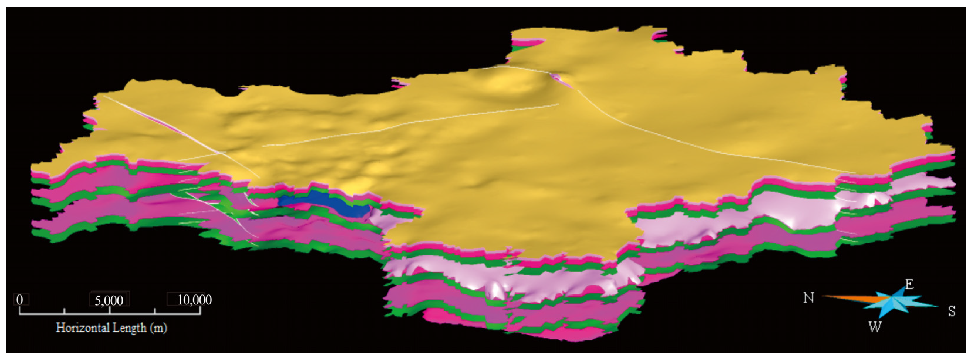
4.1. Subsurface Stratigraphy

A total of six categories (artificial ground, clayey silt, clay, silty clay, silt–fine sand, medium–coarse sand/gravel) was generalized to draw-up cross-sections. In total, 476 boreholes and 44 cross-sections were integrated into the 3D structural model (layer model), which contained 10 stratigraphic surfaces (markers) up to 50 m from the ground (Figure 6, Figure 7, Figure 8 and Figure 9). The continuity of the depositional units was interrupted locally by active faults or erosional boundaries.

Subsoil deposits up to 50 m beneath the Tongzhou area were divided into 10 major geological layers in general. Main layers were then grouped into assemblages representing three cyclothems of alluvial deposits (for example, cyclothems on Figure 4). The 3D model showed spatial stratigraphic structures comprising cyclic sequences of clay, interbedded silt, sand, and gravel with lenses (Figure 7, Figure 8 and Figure 9).

The upper ~17 m of alluvial deposits (i.e., the first cyclothem) comprised layers of artificial ground, interbedded units of silt and clay, sand, and gravel. The thickness of the gravel was around 3 m, locally identified in the north and absent from the central and southern parts of the area. Following gravel, a layer of sand with a thickness of around 9 m, described as silt or fine-grained sand, comprising feldspar, quartz, mica, iron oxides, and a few organic materials, was observed throughout the entire area. A thin layer of silty clay was intercalated in the southeastern area (Figure 7). Overlying the sand, a succession of clay could be found, identified as silty clay with heavy silty clay locally developing. The upper silt layer overlaid the silty clay, with thicknesses up to 7 m (3 m on average), and it was interpreted to be clayey silt containing mica, iron oxides, and turquoise, and silty clay lenses were locally intercalated. Following the upper clayey silt, 1–2 m of artificial ground was identified throughout the whole area (Figure 8).

The second cyclothem comprised units of clay, silt, and sand (Figure 9a). A thick layer of sand (i.e., the second sand layer) lay on the bottom of the cycle and was identified as fine-grained and medium–coarse grained sand, containing few organic materials and gravel lenses. Following the sand, an about 4.5 m thick layer of clay occurred throughout the entire area and was identified as silty clay. A unit of silt overlaid the clay, with an average thickness of approximately 4 m, described as clayey silt, which was found in the southern half of the district.

The third cyclothem was characterized by widely-distributed units of silty clay and fine-grained sand (Figure 9b). The former mainly comprised brownish yellow or greyish-yellow silty clay, medium to stiff, with thicknesses typically ranging from 1 to 10 m (4.7 m on average), commonly containing minerals such as mica, turquoise, as well as organic or iron oxide materials. The latter consisted of brown–yellow or grey fine-grained sand, dense and saturated, with a mean thickness of around 9.6 m. Minerals included feldspar, quartz, mica, as well as organic materials. Lenses of gravel, coarse-grained sand, or clayey silt were also identified occasionally within the thick unit. Figure 10 shows the distribution of subsurface layers along the NS12 cross-section.

4.2. Three-Dimensional Property Model

Based on the above 3D structural model, Reservoir Properties workflow (SKUA-GoCAD) was then adopted to construct property models that can be attributed with properties involving physical and geotechnical parameters such as natural water content (w%), initial void ratio (e), and compression modulus (Es). For example, Figure 11 exhibits the distribution of the liquid limit based on the 3D property model.

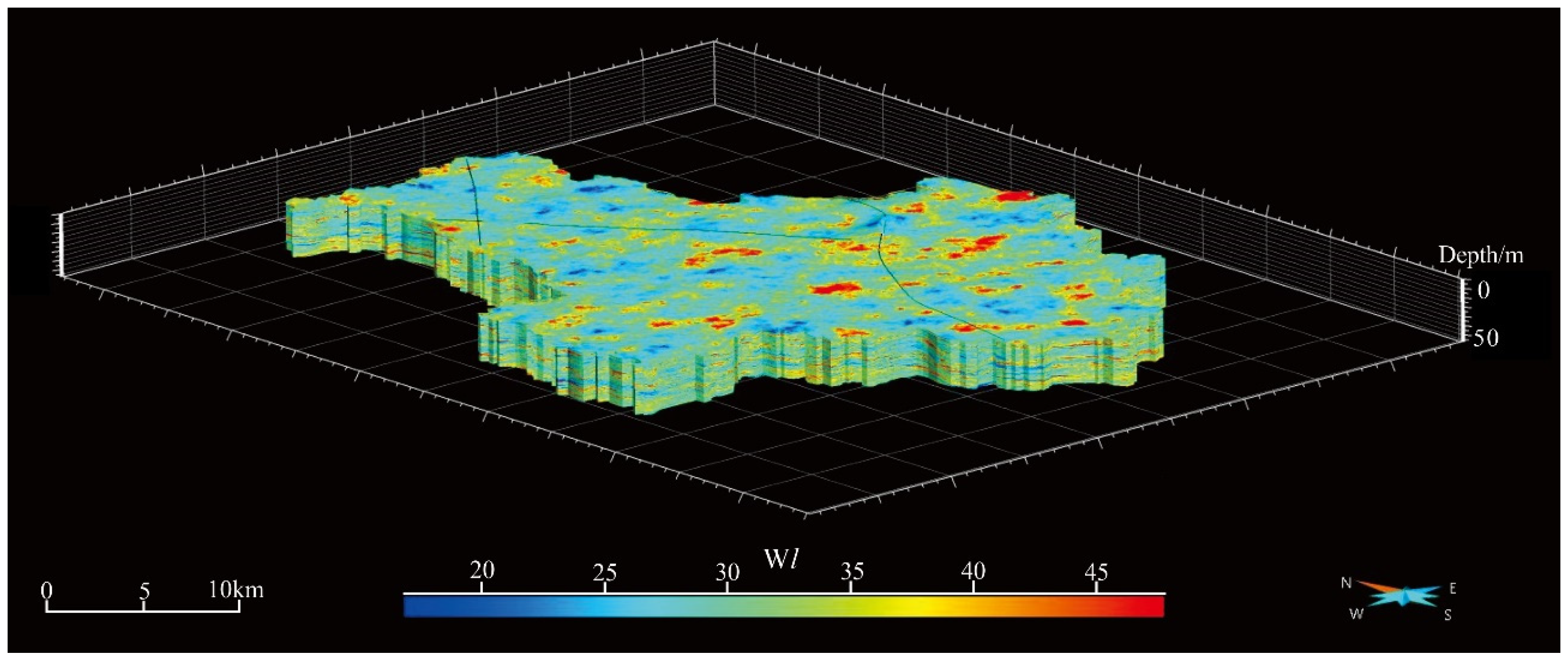
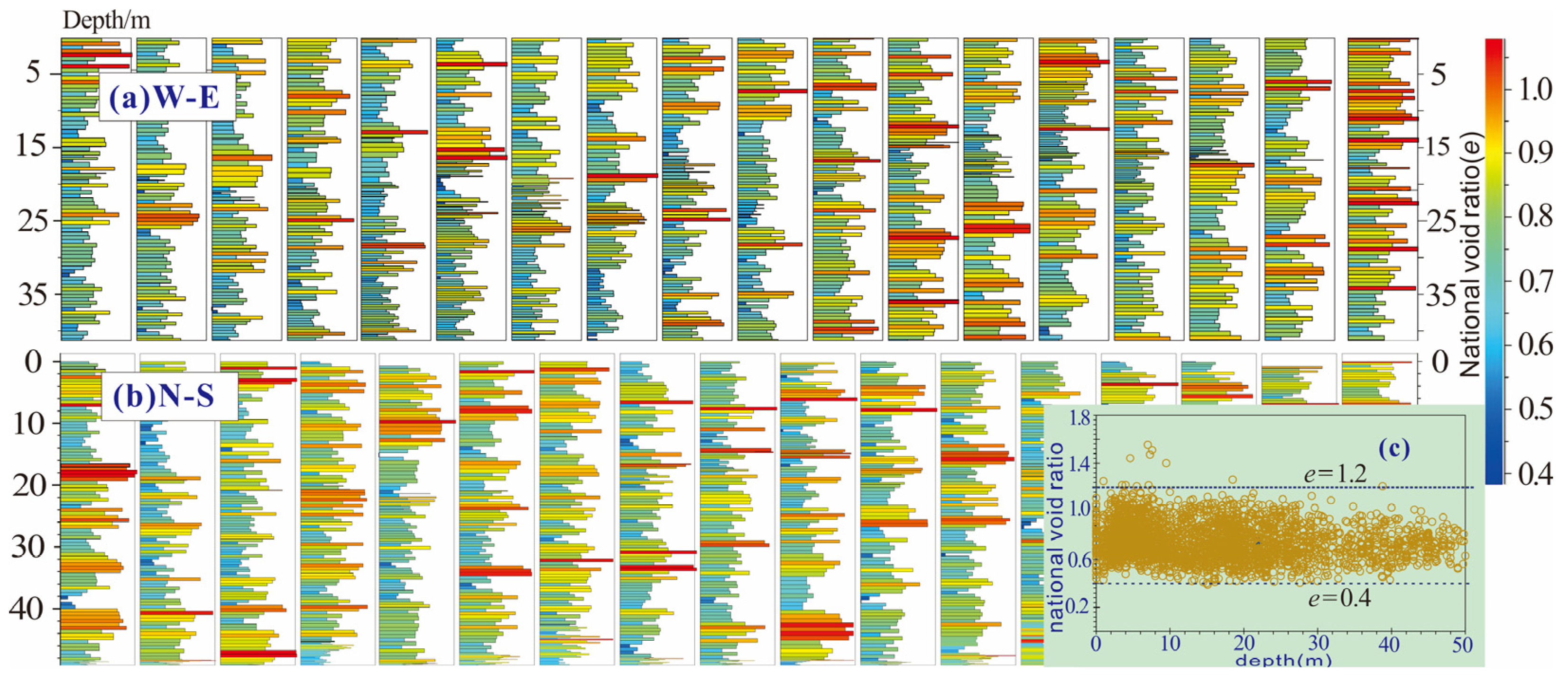
4.2.1. Water Content (w%) and Initial Void Ratio (e)

Water content varied from 6.5% to 53.1% with an average value of around 24.8% for subsoils at depths up to 50 m in the study area, with no trend related to the depth of the samples or their lithologies (Figure 12). Figure 12c shows all measured results of soil water content and indicates that w values were mainly concentrated in the range of 20–35%, which is also in accordance with the information Figure 12a,b indicates. While the national void ratio changed from 0.4 to 1.2 (Figure 13) with a mean value of about 0.8, vertically, Figure 14 exhibits w and e values of three silty clay units derived from the 3D property model. There was a tendency for silty clay at deeper depth to have a lower national void ratio in the study area, whereas the water contents were within similar intervals for three units.

4.2.2. Compression Modulus (Es)

Figure 15 shows the Es-attributed 3D geological model. It reveals that Es values increased gradually as depth increased. To determine the depth-related distribution features of the compression modulus in the vertical direction, diverse depth intervals of 0–10 m, 10–17 m, 17–35 m, and >35 m based on local cyclic depositional features described above are further discussed separately.

The Es values varied from 2 MPa to 27 MPa with an average value of 6.4 MPa for silty clay at depths up to 10 m, from 4 to 33 MPa with a mean value of 9.6 MPa for the unit at 10–17 m depths, and from 5 to 47 MPa (average of 11.8 MPa) for silty clay at depths between 17 m and 35 m and 6 to 54 MPa (16.8 MPa on average) for the unit that lies at 35–50 m. As shown in Figure 16, silty clay at shallow depths (0–10 m), with a compression modulus generally lower than 7.5 Ma, was identified as a medium-to-high compressibility unit (Es ≤ 7.5, Beijing Geotechnical Institute and Beijing Institute of Architectural Design, 2017, DBJ 11–501–2009). For layers at depth intervals of 10–17 m and 17–35 m, with Es values normally concentrated in the range of 4–7.5 Mpa and 7.5–11 Mpa (Figure 16), respectively, they were thus considered as having medium-to-high compressibility and low to medium-low compressibility, while low compressibility silty clay dominated across 35–50 m depth intervals. Moreover, as seen from Figure 17 (i.e., compression modulus at varying depths derived from 3D property model), Es of silty clay units was heterogeneous, for example, at the depth of 10 m, and a small area in the central part of the region showed slightly higher Es values than did the surroundings at the same depth, with relatively lower compressibility.

5. Applications

The integrated geological information combined within the 3D model has become a useful tool to visualize the depth and geometry variations below ground to characterize a large variety of properties that the units contain and hence to evaluate the underground geological conditions, for instance, to optimize the planning and development of subsurface structures in urban areas. Typically, 3D subsurface modeling outputs are not utilized directly in the urban planning process but form the basis for applied models [57], for example, dynamic monitoring models, and for information on geotechnical and geochemical subsurface properties. Geological and geotechnical applications based on the attributes each unit was parametrized with are mainly discussed in this work.

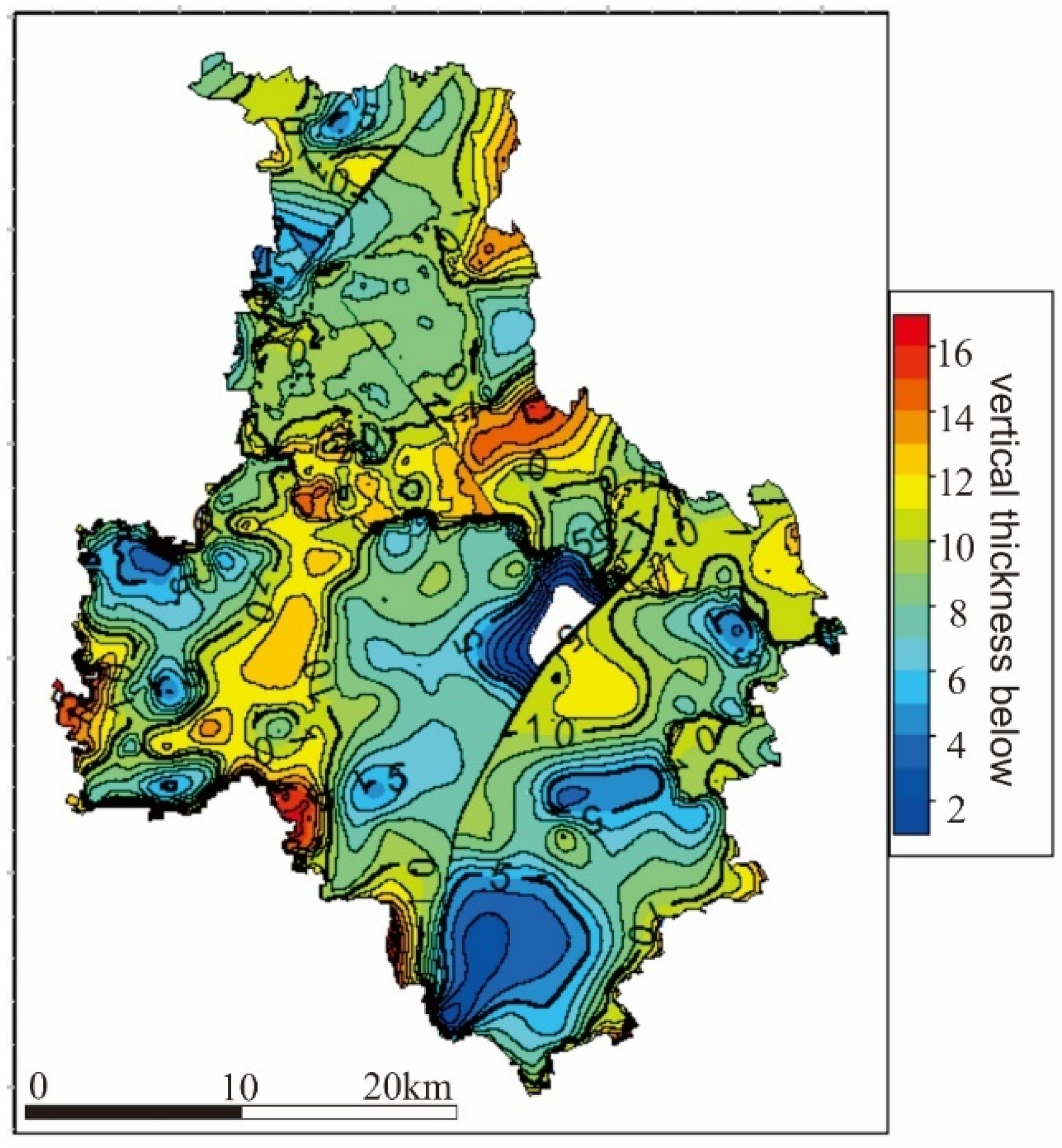
5.1. Depth Variations

Before construction and other tunneling development, 3D modeling can predict the depth of potentially suitable foundation layers (

Table 1. Interpreted thicknesses of various units derived from the 3D geological model and borehole data.

Geological Units		Unit Thickness (m)
		Derived from the 3D Model						Borehole Data
		Max	Min	Mean	Std. Dev	Median	Variance	Max	Min	Mean	Std. Dev
Artificial ground		3.00	0	1.31	0.20	1.35	0.04	4.10	0.28	1.12	0.56
The first cyclothem	clayey silt 22	7.24	0	2.95	0.47	3.04	0.22	10.1	0.4	2.72	1.47
	silty clay 23	15.77	0	3.65	0.67	3.75	0.45	10.5	0.3	3.31	1.81
	sand 24	40.99	0	9.08	2.77	9.08	7.66	21.1	0.1	6.68	3.96
	gravel 25	10.68	0	2.63	1.58	2.44	2.49	11.1	1.0	4.43	2.42
The second cyclothem	clayey silt 32	33.38	0	4.25	2.30	3.99	5.30	12.8	0.5	3.92	2.30
	silty clay 33	37.45	0	4.49	0.97	4.43	0.94	12.8	0.5	4.66	2.60
	sand 34	31.04	0	11.79	1.92	11.97	3.67	23.0	1.5	11.88	3.66
The third cyclothem	silty clay 43	23.67	0	4.67	0.78	4.82	0.61	13.9	0.4	5.08	1.82
	sand 44	38.42	0	9.61	1.73	9.68	3.00	21.7	0.7	8.90	2.66

), for example, by showing the possible distribution of sand that has a significant effect on groundwater control, by exhibiting the distribution of stable and continuous clay units that affect the potential location of tunnels.

As indicated above, ten major units were identified in the Tongzhou area, thickness maps of which could be exported from the model, such as a thickness map of the first sand layer (Unit 24), which was continuous with an average thickness of around 9 m (Figure 18) and that is widely distributed in the in Tongzhou area. Base depths of three silty clay units were indicated to be at around 8 m, 28 m, and 45 m, respectively, as derived from the model.

Additionally, the stratigraphic structure is identified as one geological indicator to assess the potential uses of UUS based on its suitability. We summarized three types of structures (

Table 2. Stratigraphic structure is identified as one of the UUS evaluation indicators (adapted after Refs. [59,60]).

Stratigraphic Structures	Sample Images	Characteristics
single-layered		Homogeneous lithology
double-layered		Two major layers; lenses may develop locally within major units; heterogeneous lithology and property across two units
multilayered		Multilayers, containing interbedded layers or lenses, heterogeneous in both lithologies and properties

) in the project titled Standard for Geological Assessment on Urban Underground Space Resources in Beijing City (DB11/T 1895—2021, Beijing Institute of Geological Survey, 2022). The weight of this indicator was then calculated using the fuzzy mathematical method, as do other basic geological indicators, such as geotechnical properties. However, for other constraints, for example, active faults, subsidence, sand liquefaction, karst collapse, etc., weights are determined based on the analytic hierarchy process (AHP) [58]. Such an approach is consistent with the evaluation model described by He et al. [59].

In the study area, a multilayered structure was interpreted following the 3D model in the depth interval of 0–50 m, with double-layered developing locally or at a particular depth interval, demonstrating the heterogeneous feature of local subsoils, with relatively lower quantification result than that of a single-layered zone (Table 2).

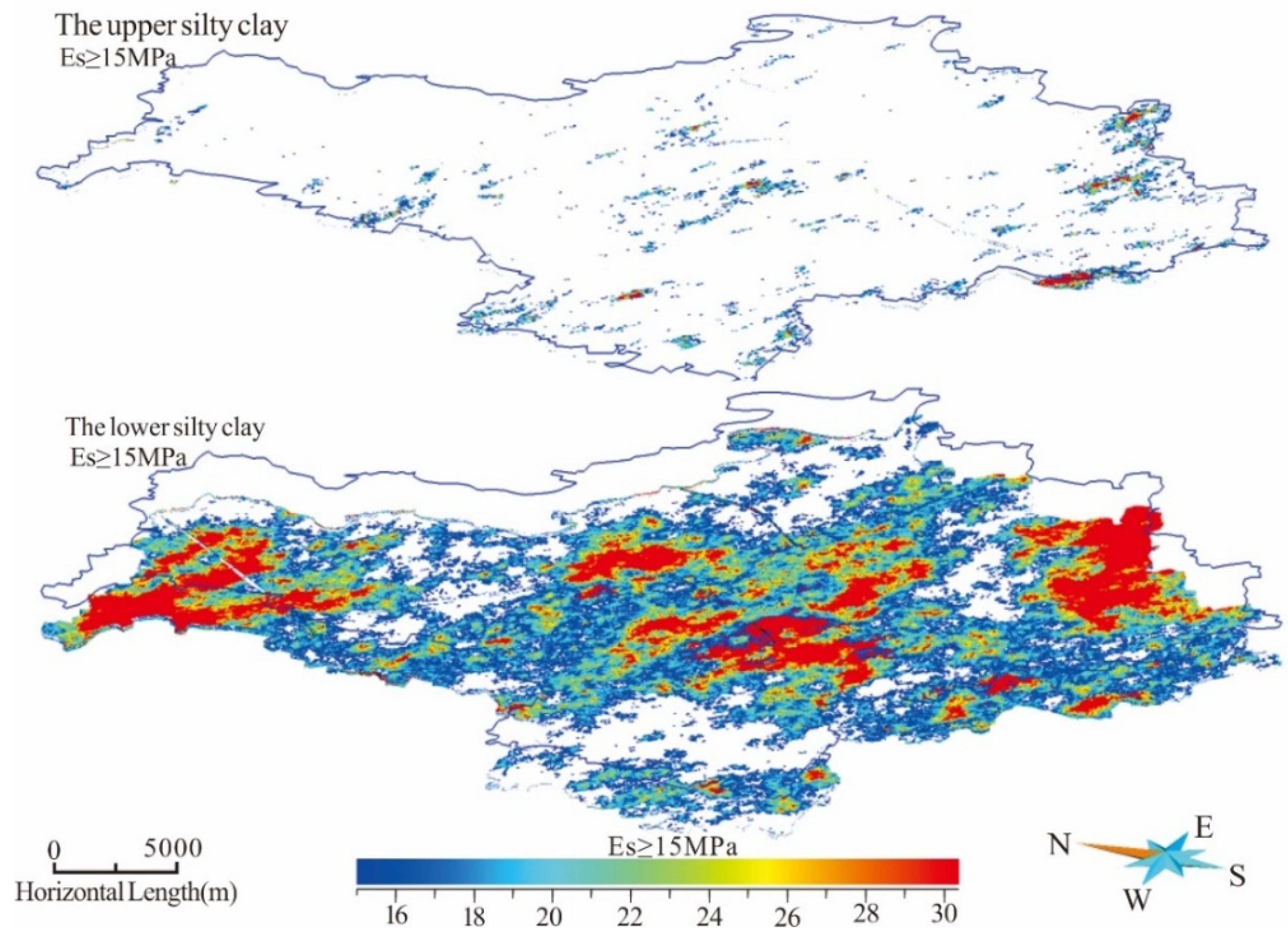
5.2. Es Distribution

Another important application of the 3D model is its potential to characterize a large variety of properties that the units contain. Analyses of engineering properties that are heterogeneously distributed within geological units play a role in UUS evaluation [6,9,61].

Geotechnical properties are adopted as one indicator for evaluation, as described before. The compression modulus is included in the Standard for Geological Assessment on Urban Underground Space Resources in Beijing City (DB11/T 1895—2021, Beijing Institute of Geological Survey, 2022) considering its influence on engineering geological conditions. Its quantification results in this work are shown in

Table 3. Es values and stratigraphic structure considered as evaluation indicators for UUS suitability. The quantification result is divided into three intervals containing 6–10, 3–6, and 0–3, representing simple, medium, and complicated geological conditions respectively.

Indicator	Evaluation Criteria
	6–10	3–6	0–3
Geological conditions	simple	medium	complex
Es values (MPa)	≥15	4–15	≤4
Stratigraphic structure	single-layered	double-layered	multilayered

* Note: Es values and stratigraphic structures are merely two of the evaluating indicators according to the Standard for Geological Assessment on Urban Underground Space Resources in Beijing City (DB11/T 1895—2021, Beijing Institute of Geological Survey, 2022).

. Evaluation criteria are divided into three intervals containing 6–10, 3–6, and 0–3 representing simple, medium, and complicated geotechnical conditions, respectively. Three spatial zones divided by Es values are then calculated based on the 3D property model, and the compression modulus of two silty clay units with values larger than 15 is interpreted as simple with a score interval of 6–10, as shown in Figure 19.

5.3. Dynamic Monitoring Model

The dynamic monitoring model is achieved by incorporating monitoring data such as values acquired from the distributed fiber-optic monitoring systems throughout a time interval into the 3D geological model. Figure 20 shows the compression deformation of the units (sand and silty clay) at a depth interval of 30–40 m throughout the period from 18/7/2019 to 22/9/2020. The target layer exhibits low compressibility with an average vertical deformation of 0.97 mm from July 2019 to September 2020 (annual report on geological safety monitoring of underground space resources at Tongzhou monitoring station in Beijing, 2020), which is much lower than that of upper silty clay.

Taking the above Es data and thickness variations into consideration, the layer of sand and silty clay at depths between 30 m to 40 m seemed to be suitable for underground construction from the aspect of vertical stability in the study area. This will be further explored in an ongoing study using 3D geological models as a framework to construct a dynamic monitoring model in the Tongzhou area.

6. Conclusions

The main goal of this study was to present an efficient and practical framework of 3D geological modeling of Quaternary sedimentary in the urban area and discuss the potential applications. Taking Tongzhou district as a typical example, 476 boreholes (40 new drilled deeper boreholes and 436 existing engineering boreholes) were utilized to provide new insight into shallow sedimentary. This insight was then used in 3D geological modeling of the shallow subsurface and UUS evaluation. The framework and analyses in this study contributed to the following applications: (1) High-quality information from new boreholes and existing engineering boreholes were used to define stratigraphy and built cross-sections. (2) The resulting geological model (up to 50m beneath Tongzhou area) shows many details of the shallow subsurface. This includes 10 major layers that were grouped into three cyclothems representing cyclic sequences of clay, interbedded silt, sand, and gravel with variable quantities of lenses. (3) The new model was used as a tool to visualize the depth and geometry variations below ground and to characterize a large variety of properties (for example, the compression modulus analyzed in this study) that each unit contains, and then to evaluate the underground geological conditions. (4) An analysis of a dynamic monitoring model based on the resulting 3D model indicated that the geological units (sand and silty clay) at depths between 30 m to 40 m, with an average vertical deformation of 0.97 mm from July 2019 to September 2020, are suitable for underground construction, from the perspective of vertical stability in the study area. This will be further explored in an ongoing study using the 3D geological model as a framework for a dynamic monitoring model in the Tongzhou area.

References

1. Wang, C.S.; Zhou, C.H.; Peng, J.B.; Fan, J.; Zhu, H.H.; Li, X.Z.; Cheng, G.H.; Dai, C.S.; Xu, N.X. A discussion on high-quality development and sustainable utilization of China’s urban underground space in the new era. Earth Sci. Front. 2019, 26, 1–8, (In Chinese with English abstract). [Google Scholar]
2. Aldiss, D.T.; Black, M.G.; Entwisle, D.C.; Page, D.P.; Terrington, R.L. Benefits of a 3D geological model for major tunnelling works: An example from Farringdon, east–central London, UK. Q. J. Eng. Geol. Hydrogeol. 2012, 45, 405–414. [Google Scholar] [CrossRef]
3. Andersen, T.R.; Poulsen, S.E.; Pagola, M.A.; Medhus, A.B. Geophysical mapping and 3D geological modelling to support urban planning: A case study from Vejle, Denmark. J. Appl. Geophys. 2020, 180, 104130. [Google Scholar] [CrossRef]
4. Costa, A.L.; Sousa, R.L.; Einstein, H.H. Probabilistic 3D alignment optimization of underground transport infrastructure integrating GIS-based subsurface characterization. Tunn. Undergr. Space Technol. 2017, 72, 233–241. [Google Scholar] [CrossRef]
5. Culshaw, M.G. From concept towards reality: Developing the attributed 3D geological model of the shallow subsurface. Q. J. Eng. Geol. Hydrogeol. 2005, 38, 231–284. [Google Scholar] [CrossRef]
6. Zhou, D.K.; Li, X.Z.; Wang, Q.; Wang, R.; Wang, T.D.; Gu, Q.; Xin, Y.X. GIS-based urban underground space resources evaluation toward three-dimensional land planning: A case study in Nantong, China. Tunn. Undergr. Space Technol. 2019, 84, 1–10. [Google Scholar] [CrossRef]
7. Dong, M.; Neukum, C.; Hu, H.; Azzam, R. Real 3D geotechnical modeling in engineering geology: A case study from the inner city of Aachen, Germany. Bull. Eng. Geol. Environ. 2015, 74, 281–300. [Google Scholar] [CrossRef]
8. Maio, R.D.; Paola, C.D.; Forte, G.; Piegari, E.; Urciuoli, G. An integrated geological, geotechnical and geophysical approach to identify predisposing factors for flowslide occurrence. Eng. Geol. 2020, 267, 105473. [Google Scholar] [CrossRef]
9. Hou, W.; Yang, L.; Deng, D.; Ye, J.; Clarke, K.; Yang, Z.; Zhuang, W.; Liu, J.; Huang, J. Assessing quality of urban underground spaces by coupling 3D geological models: The case study of Foshan city, South China. Comput. Geosci. 2016, 89, 1–11. [Google Scholar] [CrossRef]
10. Rienzo, F.D.; Oreste, P.; Pelizza, S. Subsurface geological-geotechnical modelling to sustain underground civil planning. Eng. Geol. 2008, 96, 187–204. [Google Scholar] [CrossRef]
11. Rienzo, F.D.; Oreste, P.; Pelizza, S. 3D GIS Supporting Underground Urbanisation in the City of Turin (Italy). Geotech. Geol. Eng. 2009, 27, 539–547. [Google Scholar] [CrossRef]
12. Royse, K.R.; Rutter, H.K.; Entwisle, D.C. Property attribution of 3D geological models in the Thames Gateway, London: New ways of visualising geoscientific information. Bull. Eng. Geol. Environ. 2008, 68, 1–16. [Google Scholar] [CrossRef]
13. Breunig, M. An approach to the integration of spatial data and systems for a 3D geo-information system. Comput. Geosci. 1999, 25, 39–48. [Google Scholar] [CrossRef]
14. Lemon, A.M.; Jones, N.L. Building solid models from boreholes and user-defined cross-sections. Comput. Geosci. 2003, 29, 547–555. [Google Scholar] [CrossRef]
15. Wu, Q.; Xu, H.; Zou, X.K. An effective method for 3D geological modeling with multi-source data integration. Comput. Geosci. 2005, 31, 35–43. [Google Scholar] [CrossRef]
16. Maccormack, K.; Arnaud, E.; Parker, B.L. Using a Multiple Variogram Approach to Improve the Accuracy of Subsurface Geological Models. Can. J. Earth Sci. 2017, 55, 786–801. [Google Scholar] [CrossRef]
17. Touch, S.; Likitlersuang, S.; Pipatpongsa, T. 3D geological modelling and geotechnical characteristics of Phnom Penh subsoils in Cambodia. Eng. Geol. 2014, 178, 58–69. [Google Scholar] [CrossRef]
18. Turner, A.K. Challenges and trends for geological modelling and visualisation. Bull. Eng. Geol. Environ. 2006, 65, 109–127. [Google Scholar] [CrossRef]
19. Zhang, F.; Zhu, H.H.; Ning, M.X. Modeling method of 3D strata suitable for massive data. Chin. J. Rock Mech. Eng. 2006, 25, 3305–3310, (In Chinese with English abstract). [Google Scholar]
20. Zhu, L.F.; Zhang, C.J.; Li, M.J.; Pan, X.; Sun, J.Z. Building 3D solid models of sedimentary stratigraphic systems from borehole data: An automatic method and case studies. Eng. Geol. 2012, 127, 1–13. [Google Scholar] [CrossRef]
21. Caumon, G.; Gray; Antoine, C.; Titeux, M.-O. Three-Dimensional Implicit Stratigraphic Model Building From Remote Sensing Data on Tetrahedral Meshes: Theory and Application to a Regional Model of La Popa Basin, NE Mexico. IEEE Trans. Geosci. Remote Sens. 2013, 51, 1613–1621. [Google Scholar] [CrossRef]
22. Caumon, G.; Collon-Drouaillet, P.; Veslud, C.L.C.D.; Viseur, S.; Sausse, J. Surface-Based 3D Modeling of Geological Structures. Math. Geosci. 2009, 41, 927–945. [Google Scholar] [CrossRef] [Green Version]
23. Frank, T.; Tertois, A.L.; Mallet, J.L. 3D-reconstruction of complex geological interfaces from irregularly distributed and noisy point data. Comput. Geosci. 2007, 33, 932–943. [Google Scholar] [CrossRef]
24. Jørgensen, F.; Høyer, A.-S.; Sandersen, P.B.E.; He, X.L.; Foged, N. Combining 3D geological modelling techniques to address variations in geology, data type and density—An example from Southern Denmark. Comput. Geosci. 2015, 81, 53–63. [Google Scholar] [CrossRef]
25. Pellerin, J.; Lévy, B.; Caumon, G.; Botella, A. Automatic surface remeshing of 3D structural models at specified resolution: A method based on Voronoi diagrams. Comput. Geosci. 2014, 62, 103–116. [Google Scholar] [CrossRef]
26. Wang, Z.G.; Qu, H.G.; Wu, Z.X.; Yang, H.J.; Du, Q.L. Formal representation of 3D structural geological models. Comput. Geosci. 2016, 90, 10–23. [Google Scholar] [CrossRef]
27. Gallerini, G.; Donatis, M. 3D modeling using geognostic data: The case of the low valley of Foglia river (Italy). Comput. Geosci. 2009, 35, 146–164. [Google Scholar] [CrossRef]
28. Travelletti, J.; Malet, J.P. Characterization of the 3D geometry of flow-like landslides: A methodology based on the integration of heterogeneous multi-source data. Eng. Geol. 2012, 128, 30–48. [Google Scholar] [CrossRef]
29. Zhu, L.F.; Li, M.J.; Li, C.L.; Shang, J.G.; Chen, G.L.; Zhang, B.; Wang, X.F. Coupled modeling between geological structure fields and property parameter fields in 3D engineering geological space. Eng. Geol. 2013, 167, 105–116. [Google Scholar] [CrossRef]
30. Collon, P.; Steckiewicz-Laurent, W.; Pellerin, J.; Laurent, G.; Caumon, G.; Reichart, G.; Vaute, L. 3D geomodelling combining implicit surfaces and Voronoi-based remeshing: A case study in the Lorraine Coal Basin (France). Comput. Geosci. 2015, 77, 29–43. [Google Scholar] [CrossRef]
31. Price, S.J.; Terrington, R.L.; Busby, J.; Bricker, S.; Berry, T. 3D ground-use optimisation for sustainable urban development planning: A case-study from Earls Court, London, UK. Tunn. Undergr. Space Technol. 2018, 81, 144–164. [Google Scholar] [CrossRef]
32. Rodríguez, A.A.; Kuhlmann, U.; Marschall, P. 3D modelling of the Excavation Damaged Zone using a Marked Point Process technique. Geomech. Energy Environ. 2018, 17, 29–46. [Google Scholar] [CrossRef]
33. Ye, S.; Luo, Y.; Wu, J.; Yan, X.; Wang, H.; Jiao, X.; Teatini, P. Three-dimensional numerical modeling of land subsidence in Shanghai, China. Hydrogeol. J. 2016, 24, 695–709. [Google Scholar] [CrossRef]
34. May, M.E.; Dlala, M.; Chenini, I. Urban geological mapping: Geotechnical data analysis for rational development planning. Eng. Geol. 2010, 116, 129–138. [Google Scholar] [CrossRef]
35. Rohmer, O.; Bertrand, E.; Mercerat, E.D.; Régnier, J.; Alvarez, M. Combining borehole log-stratigraphies and ambient vibration data to build a 3D Model of the Lower Var Valley, Nice (France). Eng. Geol. 2020, 270, 105588. [Google Scholar] [CrossRef]
36. Burke, H.; Mathers, S.J.; Williamson, J.P.; Thorpe, S.; Ford, J.; Terrington, R.L. The London Basin Superficial and Bedrock LithoFrame 50 Model; British Geological Survey: Nottingham, UK, 2014. [Google Scholar]
37. Ford, J.R.; Burke, H.; Royse, K.R.; Mathers, S.J. The 3D Geology of London and the Thames Gateway: A Modern Approach to Geological Surveying and Its Relevance in the Urban Environment; British Geological Survey: Nottingham, UK, 2008. [Google Scholar]
38. MacCormack, K.E.; Berg, R.C.; Kessler, H.; Russell, H.A.J.; Thorleifson, L.H. 2019 Synopsis of Current Three-Dimensional Geological Mapping and Modeling in Geological Survey Organizations; AER/AGS Special Report 112; Alberta Energy Regulator/Alberta Geological Survey: Edmonton, AB, Canada, 2019. [Google Scholar]
39. Høyer, A.S.; Klint, K.E.S.; Fiandaca, G.; Maurya, P.K.; Christiansen, A.V.; Balbarini, N.; Bjerg, P.L.; Hansen, T.B.; Mller, I. Development of a high-resolution 3D geological model for landfill leachate risk assessment. Eng. Geol. 2019, 249, 45–59. [Google Scholar] [CrossRef]
40. Chen, Q.; Liu, G.; Ma, X.; Li, X.; He, Z. 3D stochastic modeling framework for Quaternary sediments using multiple-point statistics: A case study in Minjiang Estuary area, Southeast China. Comput. Geosci. 2019, 136, 104404. [Google Scholar] [CrossRef]
41. Cai, X.M.; Luan, Y.B.; Guo, G.X.; Liang, Y.N. 3D Quaternary geological structure of Beijing plain. Geol. China 2009, 36, 1021–1029, (In Chinese with English abstract). [Google Scholar]
42. Zhi, C.; Chen, H.; Li, P.; Ma, C.; Zhang, J.; Zhang, C.; Wang, C.; Yue, X. Spatial distribution of arsenic along groundwater flow path in Chaobai River alluvial–proluvial fan, North China Plain. Environ. Earth Sci. 2019, 78, 259. [Google Scholar] [CrossRef]
43. Che, Z. A study of the fault activity in the capital circle. North China Earthq. Sci. 1993, 11, 23–34. [Google Scholar]
44. Jiang, W.L.; Hou, Z.H.; Xie, X. Research on paleoearthquakes in Jiuxian trenches across Nankou-Sunhe fault zone in Changping County of Beijing plain. Sci. China 2002, 45, 160–173. [Google Scholar] [CrossRef]
45. Zhang, S.M.; Wang, D.D.; Liu, X.D.; Zhang, G.H.; Zhao, J.X.; Luo, M.H.; Ren, J.J.; Wang, R.; Zhang, Y. Using borehole core analysis to reveal Late Quaternary paleoearthquakes along the Nankou-Sunhe Fault, Beijing. Sci. China Ser D Earth Sci. 2008, 51, 1154–1168. [Google Scholar] [CrossRef]
46. Huang, M.; Ninic, J.; Zhang, Q. BIM, machine learning and computer vision techniques in underground construction: Current status and future perspectives. Tunn. Undergr. Space Technol. 2021, 108, 103677. [Google Scholar] [CrossRef]
47. He, H.H.; Jing, H.; Xiao, J.Z.; Zhou, Y.X.; Liu, Y.; Li, C. 3D geological modeling and engineering properties of shallow superficial deposits: A case study in Beijing, China. Tunn. Undergr. Space Technol. 2020, 100, 103390. [Google Scholar] [CrossRef]
48. Michel, D.; Roger, A. Geostatistical Ore Reserve Estimation; Elsevier Scientific Pub. Co.: Amsterdam, The Netherland, 1977. [Google Scholar]
49. Isaaks, E.H.; Srivastava, R.H. An Introduction to Applied Geostatistics; Oxford University Press: New York, NY, USA, 1989. [Google Scholar]
50. Krige, D.G. A statistical approach to some basic mine valuation problems on the Witwatersrand. J. South Afr. Inst. Min. Metall. 1952, 52, 119–139. [Google Scholar]
51. Triantafilis, J.; Odeh, I.; Mcbratney, A.B. Five Geostatistical Models to Predict Soil Salinity from Electromagnetic Induction Data Across Irrigated Cotton. Soil Sci. Soc. Am. J. 2001, 65, 869–878. [Google Scholar] [CrossRef]
52. Lloyd, C.D.; Atkinson, P.M. Assessing uncertainty in estimates with ordinary and indicator kriging. Comput. Geosci. 2001, 27, 929–937. [Google Scholar] [CrossRef]
53. Kravchenko, A.N. Influence of Spatial Structure on Accuracy of Interpolation Methods. Soil Sci. Soc. Am. J. 2003, 67, 1564–1571. [Google Scholar] [CrossRef]
54. Zimmerman, D.L.; Zimmerman, M.B. A Comparison of Spatial Semivariogram Estimators and Corresponding Ordinary Kriging Predictors. Technometrics 1991, 33, 77–91. [Google Scholar] [CrossRef]
55. Liu, D.; Wang, Z.; Zhang, B.; Song, K.; Duan, H. Spatial distribution of soil organic carbon and analysis of related factors in croplands of the black soil region, Northeast China. Agric. Ecosyst. Environ. 2006, 113, 73–81. [Google Scholar] [CrossRef]
56. Webster, R.; Oliver, M.A. Geostatistics for Environmental Scientists, Second Edition; Wiley: Chichester, UK, 2008. [Google Scholar]
57. Schokker, J.; Sandersen, P.; Beer, H.D.; Eriksson, I.; Kallio, H.; Kearsey, T.; Pfleiderer, S.; Seither, A. 3D Urban Subsurface Modelling and Visualisation—A Review of Good Practices and Techniques to Ensure Optimal Use of Geological Information in Urban Planning. COST European Cooperation in Science and Technology Sub-Urban WG2 Report. 2017. Available online: https://www.google.com.hk/url?sa=t&rct=j&q=&esrc=s&source=web&cd=&cad=rja&uact=8&ved=2ahUKEwi9suvtxPH8AhVfr1YBHSDnDOIQFnoECAkQAQ&url=https%3A%2F%2Fwww.researchgate.net%2Fpublication%2F317304360_3D_urban_subsurface_modelling_and_visualisation_-_a_review_of_good_practices_and_techniques_to_ensure_optimal_use_of_geological_information_in_urban_planning&usg=AOvVaw2M8yqT1ejj3boaKZ6frxeT (accessed on 26 January 2023).
58. Saaty, T.L. Decision making with the analytic hierarchy process. Int. J. Serv. Sci. 2008, 1, 83–98. [Google Scholar] [CrossRef]
59. He, J.; Zhou, Y.X.; Zheng, G.S.; Wang, J.M.; Liu, Y. Research on the Geological Suitability Evaluation System of Underground Space Resource Utilization in Beijing. Chin. J. Undergr. Space Eng. 2020, 16, 955–966, (In Chinese with English abstract). [Google Scholar]
60. He, J.; He, H.H.; Zheng, G.S.; Liu, Y.; Zhou, Y.X.; Xiao, J.Z.; Wang, C.J. 3D geological modelling of superficial deposits in Beijing City. Geol. China 2019, 46, 244–254, (In Chinese with English abstract). [Google Scholar]
61. Thierry, P.; Prunier-Leparmentier, A.-M.; Lembezat, C.; Vanoudheusden, E.; Vernoux, J.-F. 3D geological modelling at urban scale and mapping of ground movement susceptibility from gypsum dissolution: The Paris example (France). Eng. Geol. 2009, 105, 51–64. [Google Scholar] [CrossRef] [Green Version]
Figure 1. (a) Distribution map of alluvial fans in the Beijing plain area (adapted from [41]); (b)distribution of original and new added boreholes in the study area; (c) boreholes selected for modeling in the study area.
Applsci 13 01932 g001
Figure 2. The modeling workflow.
Applsci 13 01932 g002
Figure 3. Original boreholes and stratigraphy were recorded along the WE08 cross-section line.
Applsci 13 01932 g003
Figure 4. Lithology generalization; an example from borehole 043542-1.
Applsci 13 01932 g004
Figure 5. Cross-section lines in the study area: (a) section lines and active faults (depth of upper breakpoint <50 m). Five buried faults including the Nanyuan-Tongxian (nt) fault, Nankou-Sunhe (ns) fault, Yaoxinzhuang (yxz) fault, Zhangjiawan (zjw) fault, and Xiadian (xd) fault; (b) geological units developed along NS12 cross-section.
Applsci 13 01932 g005
Figure 6. Three-dimensional geological structures of Tongzhou District.
Applsci 13 01932 g006
Figure 7. Distribution of the upper fine-grained sand and the inside lenses.
Applsci 13 01932 g007
Figure 8. Schematic diagram showing the first cyclothem in the study area.
Applsci 13 01932 g008
Figure 9. Distribution and thickness of geological units in the study area: (a) the second cyclothem; (b) the third cyclothem.
Applsci 13 01932 g009
Figure 10. Layer distributions based on the 3D geological model. Upper: fence diagrams of the model; below: layer distributions along the NS12 cross-section.
Applsci 13 01932 g010
Figure 11. Three-dimensional geological attributed model of subsoils in Tongzhou District (liquid limit).
Applsci 13 01932 g011
Figure 12. The water content of the subsoils (a,b) in the west–east (WE18) and north–south (NS12) orientations, respectively, derived from the 3D model; (c) all measured results vs. the depth.
Applsci 13 01932 g012
Figure 13. The initial void ratio of subsoils (a,b) in west–east (WE18) and north–south (NS12) orientations, respectively; (c) all measured results vs. the depth.
Applsci 13 01932 g013
Figure 14. Three-dimensional property model of (a) water content (w%); and (b) national void ratio (e).
Applsci 13 01932 g014
Figure 15. Three-dimensional geological model of shallow superficial deposits in Tongzhou District. Upper: Es-attributed 3D geological model; below: fence diagrams of the model.
Applsci 13 01932 g015
Figure 16. Diagrams of Es values and depth intervals (1–10 m, 10–17 m,17–35 m, and >35 m) in the study area.
Applsci 13 01932 g016aApplsci 13 01932 g016b
Figure 17. Diagrams of Es values at varying depths (10 m, 23 m, 35 m, and 45 m, respectively) derived from the 3D property model.
Applsci 13 01932 g017
Figure 18. Thickness map of the first sand unit (24) derived from the 3D geological model in the study area.
Applsci 13 01932 g018
Figure 19. The upper (23) and lower silty clay units (43) with Es values larger than 15 derived from the 3D property model.
Applsci 13 01932 g019
Figure 20. Monitoring data (vertical compression) and a preliminary dynamic model of target units at one monitoring site in the study area.
Applsci 13 01932 g020