Abstract
Deep learning has been used to improve intelligent transportation systems (ITS) by classifying ship targets in interior waterways. Researchers have created numerous classification methods, but they have low accuracy and misclassify other ship targets. As a result, more research into ship classification is required to avoid inland waterway collisions. We present a new convolutional neural network classification method for inland waterways that can classify the five major ship types: cargo, military, carrier, cruise, and tanker. This method can also be used for other ship classes. The proposed method consists of four phases for the boosting of classification accuracy for Intelligent Transport Systems (ITS) based on convolutional neural networks (CNNs); efficient augmentation method, the hyper-parameter optimization (HPO) technique for optimum CNN model parameter selection, transfer learning, and ensemble learning are suggested. All experiments used Kaggle’s public Game of Deep Learning Ship dataset. In addition, the proposed ship classification achieved 98.38% detection rates and 97.43% F1 scores. Our suggested classification technique was also evaluated on the MARVEL dataset. This dataset includes 10,000 image samples for each class and 26 types of ships for generalization. The suggested method also delivered an excellent performance compared to other algorithms, with performance metrics with an accuracy of 97.04%, a precision of 96.1%, a recall of 95.92%, a specificity of 96.55%, and a 96.31% F1 score.
1. Introduction
The classification and identification of naval vessels are essential and challenging issues for the national defense and maritime security of coastal countries. These countries must constantly work to increase port efficiency and maintain a close eye on traffic to advance economically. Threats include illegal fishing, marine pollution, and piracy [1,2]. Most of these issues require a global perspective because they are not specific to particular countries. Image technology has advanced in the last few years, so the ship classification method has taken center stage for identifying and classifying ship targets.
The basic network structure of deep learning algorithms is the convolutional neural network (CNN), which has multiple layers for automatically learning key features from training data rather than complex manual feature extraction [3]. In particular, it has been reported to solve many complex tasks, such as image classification, image semantic segmentation, and image recognition and pattern analysis [4]. CNNs have recently been trained for image classification utilizing supervised learning on large-scale annotated datasets [5]. However, training image data requires the gathering of large amounts of data which is very hard and is expensive to run, especially in marine regions where there are few publicly available datasets [6,7]. The maritime domain has a lot of datasets. These datasets include object detection, tracking, and pirate detection [8], but they have not been used for maritime categorization.
In the field of marine image classification, there are a few publicly available datasets, such as the fine-grained dataset (MARVEL) Maritime Vessels [9] and the VAIS dataset [10], which includes both visible and infrared images of ships. However, the limitations in these datasets, such as the unbalanced classes and poor image quality, could lead to incorrect image categorization [11].
In [12], Dao-Duc et al. investigate a new deep convolutional neural network (DCNN). This model is considered the base model and is twice as small as the AlexNet model. The model is used for maritime vessel image classification and is helped by the advent of new processors with high processing capability and huge memory units. Additionally, with the availability of collected massive datasets [13], deep learning (DL) techniques such as DCNNs have been utilized to create vision-based classification algorithms that do not require manually created descriptors. Instead of manually constructing features, using raw photos as the input for learning may help deep learning models understand a hierarchy of different invariant properties for geometric alterations. Unprocessed data is supplied to a classification algorithm using deep learning techniques, automatically learning how to complete the classification task.
The classification performance is frequently below average if the initial parameters are applied for a small image number of the classified target for CNN training [14]. Therefore, for smaller target datasets, available transfer learning techniques can be used [15]. Transfer learning (TL) is a helpful technique for initializing a massive network with many images and classes. For these kinds of problems, ImageNet is frequently employed as the source dataset. Then, using a sizable dataset, transfer learning substitutes a new fully connected layer for the fully connected layer (or layers) of a pre-trained network. Last, a smaller target dataset is only used for training.
DL techniques have successfully trained cutting-edge CNNs for object recognition since these models perform well in a wide range of visual tasks [16]. Due to the lack of reliable methods and annotated datasets, coarse-grained image classification rather than fine-grained image classification was used as a solution [17]. Even though some of the best CNN models have been used to classify images of ships, the EfficientNetBX CNN model is not usually used with the MARVEL dataset to detect variant vessels [18].
Academics have been trying to figure out how to make a good classification system for a long time. While all the previous research has yielded promising classification outcomes, more study is required to compare and analyze various classification algorithms implemented using CNN on a dataset of visible light images. A new classification algorithm is required to further improve the precision with which ships on inland waterways can be predicted. This is for the purpose of averting inevitable collisions.
As mentioned above, the following enhancements have been made to the proposed classification system to ease the restriction. A novel CNN design has been implemented to increase the precision of ship classification systems, initially. Based on an improved and optimized CNN model, transfer learning (TL), and ensemble learning (EL) approaches, this research proposes an innovative ship classification model for ITS. The classification system is used for inland waterway collision avoidance. Eight cutting-edge CNN models are utilized when training base learners, including Xception, VGG-16, ResNet-50, Inception V3, InceptionResNetV2, DenseNet121, MobileNet, MobileNetV2, and EfficientNetB0. These models are trained using the ship classification dataset to classify and detect different kinds of ships.
In our proposed classification system, the classification accuracy of CNN learning models and the hyper-parameters of the CNN models are tweaked using a simple bio-inspired algorithm called Particle Swarm Optimization (PSO). PSO is used as a hyper-parameter optimization (HPO) technique [19]. To further enhance the ship detection performance, the underlying CNN models are combined, utilizing the ensemble procedures of confidence averaging and concatenation. The suggested ITS framework’s efficacy and efficiency are assessed using two innovative ship classification datasets. To ensure its generalizability, the improved CNN model has also been evaluated on a more generalized MARVEL dataset, consisting of over 10,000 pictures and a whole class of 26 distinct vessels. Different classification algorithms have been compared to the proposed ship classification systems.
The following are the primary contributions that this study makes:
- First, a new convolutional neural network (CNN) architecture has been employed to improve the accuracy of ship classification systems.
- For hyper-parameter-optimization HPO, a PSO is used to enhance ship classification accuracy. Further, a new method is used to classify ships successfully for inter-class identification by using CNN, transfer learning and ensemble learning.
- The proposed optimized ensemble learning method is tested on two ship classification benchmark datasets. The experimental results show efficient intra-class and ship detection, and the model’s performance is compared to existing state-of-the-art methods.
The rest of the paper is organized as follows. Section 2 introduces the related work that uses ML and DL algorithms for ship detection and classification. Section 3 presents the proposed ensemble transfer learning classification system. The experimental setup and classification results are presented in Section 4. Finally, the conclusion and future work are presented in Section 5.
2. Related Work
The primary object of ship classification is, of course, to allow for the most precise identification of ships possible. When monitoring is completed manually or using older techniques, mistakes are possible due to human error. Identifying the precise type of ship when looking at one among the many types of vessels that may be seen on a river can be challenging at times. Since this has already been shown, the problem is easy to solve by a reliable and effective network.
Multiple factors, such as changes in weather (rain, snow, and fog), natural variations in sea level (waves), and other natural elements such as rocks, coral reefs, and sandbanks, as well as the size and form of the observed objects, make it difficult to detect and identify ships automatically. Numerous pieces of research have been conducted to solve these issues, leveraging profound advancements in deep learning techniques. The creation of boat categorization datasets, featuring photos of boats automatically retrieved by the ARGOS system, which is active in Venice during the day time, is described by Bloisi et al. [20]. Zhang et al. [10] developed a gnostic field and a CNN that has already been trained on the ImageNet dataset. An accuracy of 82.4% was attained using only the gnostic field of the VAIS dataset.
Shi et al. [17] used lower and higher hierarchical level attributes to classify ship images. All accessible feature vectors were combined using DCNNs, and the output was then given to the support vector machine (SVM) classifier. They used a DL CNN to extract high-level properties and, in order to retrieve low-level attributes, they investigated Gabor filters. The accuracy rate for CNN fine-tuning with multi-scale rotation invariance properties is then demonstrated to be 88%.
Khellal et al. [21] employed the ELM (Extreme Machine Learning) method to identify ships after training a CNN system on discriminative data. They pointed out that even when regularization techniques were used, there was still a risk of overfitting due to the paucity of training data. For the categorization of maritime vessels, Leclerc et al. [22] used pre-trained CNNs in the ResNet and Inception architectural frameworks based on transfer learning and fine-tuning. Instead of constructing a CNN using random parameters, they were able to achieve classification by optimizing previously trained models using ImageNet. They achieved the highest accuracy of 78.73% on the Marvel dataset.
Yao et al. [23] investigated and compared various CNN-based ship recognition systems. Shi et al. [24] described an alternative method. In this method, a multi-feature ensemble extracts data and is built on top of the AlexNet CNN, and a two-dimensional discrete fractional Fourier transform (2D-DFrFT) is also employed.
In order to create multi-dimensional feature maps from the input picture, Ucar et al. [25] describe a deep feature extraction method based on TL that uses cascading CNN architecture. The MUTual Information (MUTInf)-based feature selection algorithm’s distributions make up a unique feature set that was created for a public ship dataset. The chosen classifier is a non-linear support vector machine (SVM) with a quadratic kernel. The suggested framework may incorporate the best feature set with a well-designed classifier to improve the effectiveness of the classification process in ship images. The proposed approach obtains an overall accuracy of 95.06% in the experiments.
A CNN classification algorithm was introduced by Leonidas [26] which can categorize five different types of ships in inland waterways, including tankers, cargo, military, carrier, cruise, and carrier ships. Based on experiments on the Game of Ship Classification dataset, the Resnet-152 pre-trained model produced the top model with an accuracy of 90.56%. In order to address the issue of a diminishing gradient, Resnet-152 was enhanced with the addition of a classification block with two fully connected layers, followed by ReLU, and a dropout layer. The technique received an F1 score of 95.81% when it was tested on the Marvel dataset.
Based on the work of Leonidas [26] and Ucar et al. [25], modifying the pre-trained model can further enhance the classification performance. To efficiently classify ship targets, we first examine several pre-trained models for accuracy and power complexity; the computation complexity is proportional to the number of model parameters. Any model system consists of a small number of parameters that will speed prediction time. The best model is optimized and modified for better classification performance. Hyper-parameter optimization is applied to the selected pre-trained CNN model to choose the precise parameters in the optimized phase. The six model hyper-parameters are (learning rate, dropout, frozen layer, number of epochs, batch size and early stop patience). Optimization is conducted using bio-inspired particle swarm optimization (PSO). Ensemble learning (EL) of the best three CNN models is utilized to enhance the classification performance further.
3. Materials and Methods
3.1. Convolutional Neural Network Structure
When it comes to problems involving the classification and recognition of images, DL models such as CNN are frequently used [6]. The target classification images can be immediately input into CNN models without requiring additional procedures involving the extraction of features and data reconstruction. A CNN consists of three main layers; convolutional layers, pooling layers, and fully connected layers [6]. By performing convolution operations in convolutional layers, it is possible to retrieve the feature patterns contained within images automatically. The complexity of the training is reduced in pooling layers by using local correlations to prevent overfitting. Local correlations can be used without losing essential features and information. All the components are linked together by fully connected layers, which are also responsible for producing the output.
Transfer learning (TL), is the process of transferring the weights of a deep neural network (DNN) model that was previously trained on one dataset to another [14]. TL is used for DL models. The TL method has been effectively used in various image processing responsibilities. The reason for using TL is that the feature patterns learned by the bottom layers of CNN models are typically generic patterns that, with a pre-trained model, can be applied to various tasks. In contrast, the features learned by the top layers of CNN models are the only features specific to a given dataset [14]. As a result, the lower layers of CNN models are versatile enough to be immediately applied to various projects.
It is possible to employ fine-tuning in the TL process of DL models to increase the efficiency of the TL method. During the process of fine-tuning, the majority of the model layers of the pre-trained model are “frozen,” which means that their weights are kept, but a few of the top layers are “unfrozen” so that the model can be re-trained on a new dataset. The learning model can update the higher-order features in the pre-trained model through fine-tuning [14]—the results better fit the target task and the dataset. The ship dataset is classified using several traditional CNN models in this article.
3.2. CNN Model
3.2.1. Classic CNN
In this section, we selected Eight CNN models; Xception [5], VGG-16 [27], ResNet-50 [28], Inception V3 [29], InceptionResNetV2 [30], DenseNet121 [31], MobileNet [32], MobileNetV2 [33], and EfficientNetB0 [18] from the common CNNs [15], and we compared their architectures and complexity using a number of experiments to determine which of these networks would be the most effective for use in the ship target detection algorithm.
The fundamental correlation will be as follows: A model with more parameters (such as learnable weights or a larger network) will run more slowly than one with fewer parameters. Additional recurring units are slower than a full-connected network, which is slower than a convolutional network, which is slower than an ordinary network, whose activation functions are more complex and, hence, slower than ones that are more straightforward, such as ReLU deeper networks, and more sluggish than shallow network connections (with the same number of parameters), as fewer tasks are completed simultaneously on a GPU.
Having enumerated a few criteria that affect the final inference time required (the amount of time it takes to construct one forward run through the network), MobileNetV2 is definitely among the quickest pre-trained models (available in Keras). The next table demonstrates that this network’s memory footprint is rather tiny, coming in at only 14 megabytes and containing approximately 3.5 million parameters. Compare this to VGG test, which had 138 million—a 40-fold increase! MobileNetV2 also has a conv layer as its primary workhorse layer. Conv layers are essentially intelligent and more compact versions of residual networks. Ten of the most advanced pre-trained models are available for use and categorization in their current state. The following models and their respective performances are outlined in Table 1:

Table 1.
CNN different pre-trained models.
3.2.2. Modified CNN
The optimum way to balance the depth, width, and resolution of a CNN is suggested in a recent article by Tan et al. [18]. With the use of their own custom-developed compound coefficient, the scientists were able to successfully scale up Mobile and ResNets. The EfficientNet CNN architecture was also introduced in the same publication. To enhance the finest ResNet-18 model, this model will be used. Their default model includes squeeze and excite blocks sporadically along with inverted residual blocks similar to Mo-bileNetV2 [6]. When using the compound coefficient’s set of formulas, this structure can be enlarged effectively.
3.3. Proposed Method
In this research, a unique optimized CNN and transfer learning-based ITS is proposed as a means of detecting a wide variety of different kinds of ship targets in interior waterways. We proposed a new classification model in order to tackle the concerns that were discussed above, regarding the accuracy of the classification system.
Figure 1 provides a high-level representation of the ship classification system that is being considered. First, the data from different classes of the ship’s images required for classification are collected. Next, the images are transformed into a training set by balancing the ship’s different classes of images. The training dataset may be expanded with the help of additional data augmentation, which is conducted in order to increase the performance of the model and its capacity to generalize.
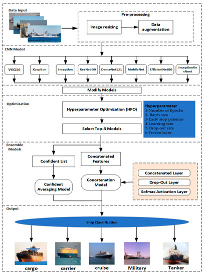
Figure 1.
Proposed architecture of modified ensemble model.
The following step involves training eight cutting-edge CNN models (VGG16, Xception, Inception, ResNet-50, DenseNet121, MobileNet, EfficientNetB0, and InceptionRes-net) using the generated image set in order to develop basic learners.
PSO, an HPO approach that is capable of automatically tuning the hyper-parameters, is used in the optimization process for the CNN models. Following that, the three CNN models with the best performance are chosen to serve as the foundation for the ensemble learning models that will be constructed. In the end, two ensemble techniques, called confidence averaging and concatenation, are used to make ensemble models for final detection.
3.3.1. Modified CNN Models
First, the models are fine-tuned with the public dataset using the eight pre-trained models (VGG16, Xception, Inception, ResNet-50, DenseNet121, MobileNet, EfficientNetB0, and InceptionResNnet) as indicated in Section 3.2. These models were based on the pre-trained ones using the ImageNet dataset. Fine tuning is applied to the pre-trained model to achieve a high level of accuracy for the classification of ships. The best model achieved among the tested pre-trained models was chosen for further processing steps; modification, optimization and ensemble.
Following the successful application of transfer learning (TL) and the fine tuning of the training of eight cutting-edge CNN models on the ship classification datasets, the top CNN model is modified by adding three additional layers. Each extra layer consists of a fully connected (FC) layer, a dropout layer and a ReLU layer. The ReLU is added to learn the new properties of our training dataset. This layer was followed by average pooling. In terms of performance, they are chosen to serve as the base learners for the ensemble models presented in the following subsection. These models are then used to construct the ensemble models. The full procedure is depicted in Figure 1.
3.3.2. Hyper-Parameter Optimization (HPO)
It is necessary to tune the hyper-parameters of CNN models to achieve a better match between the fundamental models and the selected datasets and improve the models’ performance. CNN models, in a similar way to other deep learning models, have many hyper-parameters whose values need to be tweaked to obtain optimal performance. Optimizing hyper-parameters must be conducted to select the optimal parameters which make the model work to its full potential. These hyper-parameters can be put into one of two groups: model-training hyper-parameters or model-design hyper-parameters [19]. The six selected CNN model hyper-parameters for optimization are illustrated in Table 2.
Table 2.
CNN model hyper-parameters.
The model design process is to understand how to set the model’s hyper-parameters. The six model-design hyper-parameters that are included in the TL framework and have been suggested for optimization are presented in Table 2. On the other hand, model-training hyper-parameters are utilized in order to strike a balance between the training speed and the performance of the model.
The hyper-parameters have a direct impact on the efficiency of CNN model implementations. “HPO” stands for “hyper-parameters optimization”. It is an automatic method for optimizing the hyper-parameters of machine learning or deep learning models [19].
PSO is a bio-inspired algorithm for searching for the optimal solution. PSO is a commonly used metaheuristic optimization method that discovers the optimal hyper-parameter model values via information exchange and cooperation among the individual particles in a swarm [19]. PSO is one of the optimization strategies that is utilized for HPO problems. At the beginning of the PSO process, the starting positions () and velocities () of all of the individuals in the group are determined and recorded. Following each iteration, the velocity of each particle receives an update that takes into account both the particle’s current best location () and the present global ideal position () that is shared by other individuals:
where and are random numbers between 0 and 1, the parameters w, , and are constants to the PSO algorithm, and is the position that gives the best value ever explored by particle and is that explored by all the particles in the swarm.
In conclusion, it is possible for the particles to make slow progress toward the promising regions in order to locate the global optimal. The PSO algorithm was selected for use in the proposed framework because it offers support for a wide variety of hyper-parameter types and has a low time complexity of [26].
3.3.3. Ensemble Learning Models
Following the successful application of the optimized hyper-parameters of the transfer learning (TL) and the fine-tuning to the training of cutting-edge CNN models on the ship classification datasets, the top three CNN models, in terms of performance, are chosen to serve as the base learners for the ensemble models presented in the following subsection. These models are then used to construct the ensemble models.
To improve model performance, ensemble learning (EL) can be used. In the EL technique, multiple base learning models are integrated. The new constructed model can boost classification accuracy and, hence, improve performance. Data analytics problems commonly use ensemble learning because integrating several features of variance learners usually performs better than a single one.
There are two main EL methods widely used for data analysis. Confidence averaging and concatenation. In confidence averaging EL approach, the classification probability values of base learners are combined to find the class with the highest confidence value [34]. In DL models, softmax layers can output a posterior probability list that contains the classification confidence of each class.
The confidence averaging method calculates the average classification probability of base learners for each class, and then returns the class label with the highest average confidence value as the final classification result. The confidence value of each class is calculated using the softmax function [34]:
where is the input vector in Equation (2), is classes number in the dataset, and and are the standard exponential functions for the input and output vectors, respectively.
By applying a confidence averaging method, the predicted class label obtained is denoted by:
where is the j-th base learner in Equation (3); is the number of the selected base CNN learner, and k = 3 in the proposed ship classification system; and indicates the prediction confidence of a class value in a data sample using .
Unlike the conventional voting method that only considers the class labels, confidence averaging enables the ensemble model to detect uncertain classification results and correct the misclassified samples through the use of classification confidence.
While the time complexity of the confidence averaging approach itself is merely , where is the number of instances, is the number of base CNN models, and is the number of classes, the computational cost of a whole ensemble model is dependent on the complexity of the base learners. The execution speed of the confidence averaging method is typically quite high due to the fact that and are typically quite modest.
Another ensemble method for DL models is the concatenation [35] method. In a concatenated CNN, the goal is to extract the highest-order features generated from the top dense layer of base CNN models, and then use concatenate operations to integrate all of the features into a new concatenated layer that contains all of the features. This new concatenated layer should contain all of the features. After the concatenated layer comes a drop-out layer, which is used to eliminate superfluous features, and then a softmax layer, which is used to build a new CNN model.
The concatenation process has the advantage of integrating different features of the highest order, allowing it to design models that are more efficient than the original one. On the other hand, the new model needs to be retrained on the entire dataset, increasing the time spent on the model training process. The concatenation approach’s difficulty in computation is given as is the data samples total number and is the number of features retrieved from the dense layers of the base CNN models.
4. Dataset and Classification Results
4.1. Dataset Description
A public dataset for ship classification is used to evaluate the ship classification performance. The dataset is named the Game of Deep Learning Ship dataset. The dataset mentioned can be found on Kaggle [36]. We utilized this dataset to investigate the proper classification of our proposed method. The collection contained information on five different categories of vessels: 2120 images for cargo ships, 1217 images for tankers ships, 1167 images for military ships, 916 images for carrier ships, and 832 images for cruise ships. This other ship category made it much easier to understand how various neural networks could classify inland ships and how ship classification detection was affected by the network when applying different classification network models as the system’s backbone.
The ship’s dataset images were taken from various vantage points, including multiple distances and angles, directions and atmospheric conditions, and international and offshore harbors. The collection contains a total number of 6252 photographs, some of which are RGB shots, some of which are grayscale images, and some of which have varied pixel sizes for each sort of image.
The total number of examples selected for the classification evaluation is the number of samples contained in this dataset which is greater than 832; this number is appropriate for completing the requirements for both the training and testing of models. The original dataset was partitioned into three groups with a ratio of 70% for training, 15% for testing and 15% for validation. Figure 2 shows a small selection of the images in the dataset. The classes with a sample number of more than 900 are trimmed, the purpose of trimming is to let different classes fairly contribute to the training procedure. Then, augmented images are created by replacing the original data samples.
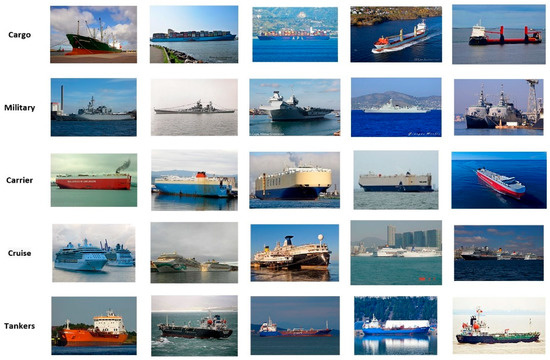
Figure 2.
Selection of random ship images from the dataset.
4.2. Evaluation Indicators
Indicators are used to evaluate the overall system classification performance of the suggested model’s network. Accuracy, precision, recall, and specificity were the metrics we utilized in this part of the evaluation of the classification algorithm we developed. Accuracy was a measurement of how accurate the model was, precision was a measurement of how well the ships were categorized, and recall was a measurement of how effectively negative samples were recognized. Specificity was the metric used to quantify how various ship classes were correctly classified. The F-measure (F1) was determined by adding the marks for accuracy and recall (8). The formulations for these metrics are as in the following equations:
In the equations of classification evaluation (4)–(7), true positive (TP) indicates a correctly classified ship, false positive (FP) indicates an incorrectly classified ship, false negative (FN) indicates a correctly classified ship for members, and true negative (TN) indicates a correctly classified ship for members in Equations (4)–(7). Both the total number of the test samples that were correctly predicted and the total number of test samples that were correctly labelled were the same.
4.3. System Process
4.3.1. Pre-Processing Phase
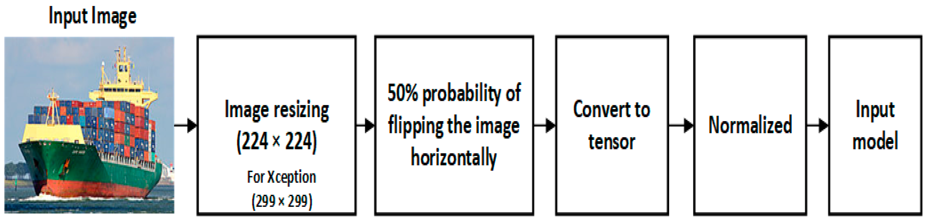
The correct preprocessing of the pictures utilized in the training of DCNNs has the potential to effectively speed up the convergence speed during the training process. Figure 3 illustrates the preprocessing techniques that were used on the data in this section. The normalized function is shown in Equation (9),
where stands for the image channel, stands for the mean, and stands for the standard deviation.
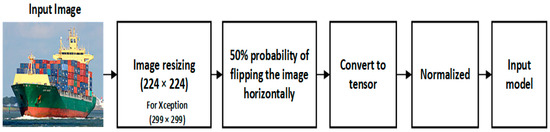
Figure 3.
Pre-processing process for input image.
4.3.2. Parameter Setting and Initialization
In order to hasten the process of training the network that was being used in this experiment, its parameters were initially set to match those of the ImageNet pretraining network. Because the categories that were utilized by ImageNet and our dataset were different from one another, the very last layer of the network required some fine tuning in order to function properly. The pretraining weights for this layer were unable to be utilized in any manner, shape, or form.
For the initial setting, the hyper-parameter settings of each network in the experiment before optimization are as follows: Image size of 224 × 224 (Xception 299 × 299), Batch Size 64, Training Learning Rate set equal to 0.001 with a Momentum Factor equal to 0.9. During the phase of the experiment, the level of accuracy achieved by the training set was measured after each epoch, and the level of accuracy achieved by the test set was measured after the training was finished.
In the beginning, the eight currently pre-trained versions (VGG16, Xception, Inception, ResNet-50, DenseNet121, MobileNet, EfficientNetB0, and InceptionResnet) were modified to the Game of Deep Learning Ship dataset in order to achieve the highest possible network performance in the suggested ship classification. The performance of a variety of different models was analyzed, and the one with the best overall performance was chosen for modification and used for the classification of the network. This helped to ensure that the results were as accurate as possible. The models were altered to ensure that they were consistent with the categories that were uncovered in the dataset that was made accessible to the public. The PyTorch framework was utilized to train these network models, and Adam was employed to maximize both the momentum and the learning rate. The cross-entropy loss function was used throughout the whole process to measure loss, and validation was completed after each epoch to see how well the network was learning while it was being trained.
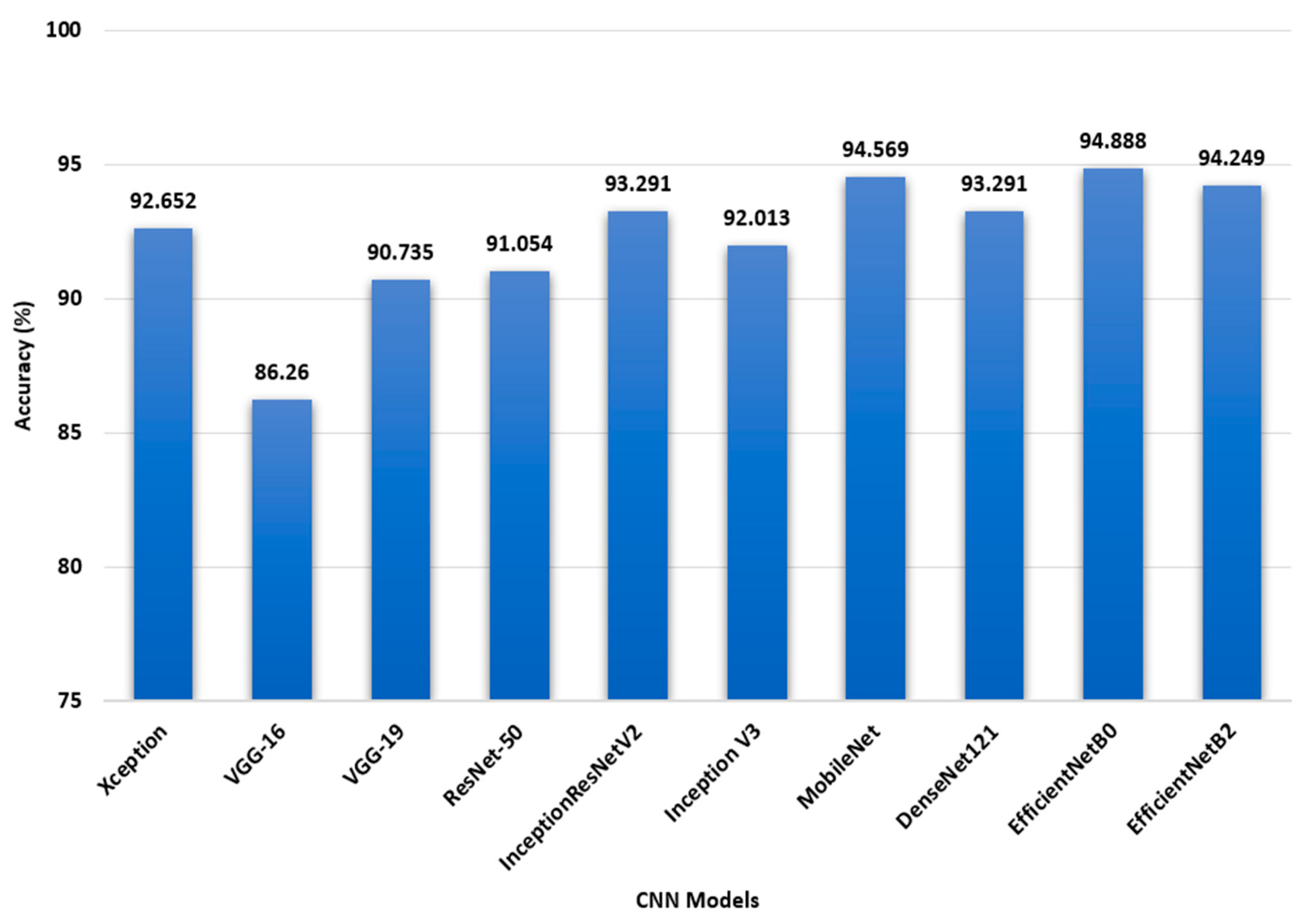
Figure 4 demonstrates that when compared to VGG16, Xception, Inception, ResNet-50, DenseNet121, MobileNet, and InceptionResnetV2, EfficientNetB0 achieved a greater level of accuracy in its predictions. The model with the lowest accuracy was VGG16, which differed by a margin of 8.62%. EfficientNetB0 had an accuracy of 94.25%, whereas InceptionResnetV2 accuracy was only 93.29%. The accuracy achieved by DenseNet121, 93.29%, was superior to that achieved by both VGG-16 and Xception. On the other hand, the Xception model achieved an accuracy of 92.65%, which is significantly better than the VGG-16 model. In addition, the accuracy of MobileNet was measured at 94.56%. Following the results of the experiment, it is hypothesized that enhancing the EfficientNetB model will result in improved accuracy and that the model will be able to be utilized for better performance results.

Figure 4.
Performance of eight CNN model on the ship classification test set.
4.4. Experiment Results and Analysis
4.4.1. Hyper-Parameter Optimization (HPO)
To construct optimal models, the major hyper-parameters of all the base CNN models in the proposed framework were optimized using PSO. The HPO process was implemented for the Game of Deep Learning Ship dataset. Table 3 illustrates the initial search range and the optimal values of the hyper-parameters.
Table 3.
CNN models Hyper-Parameter.
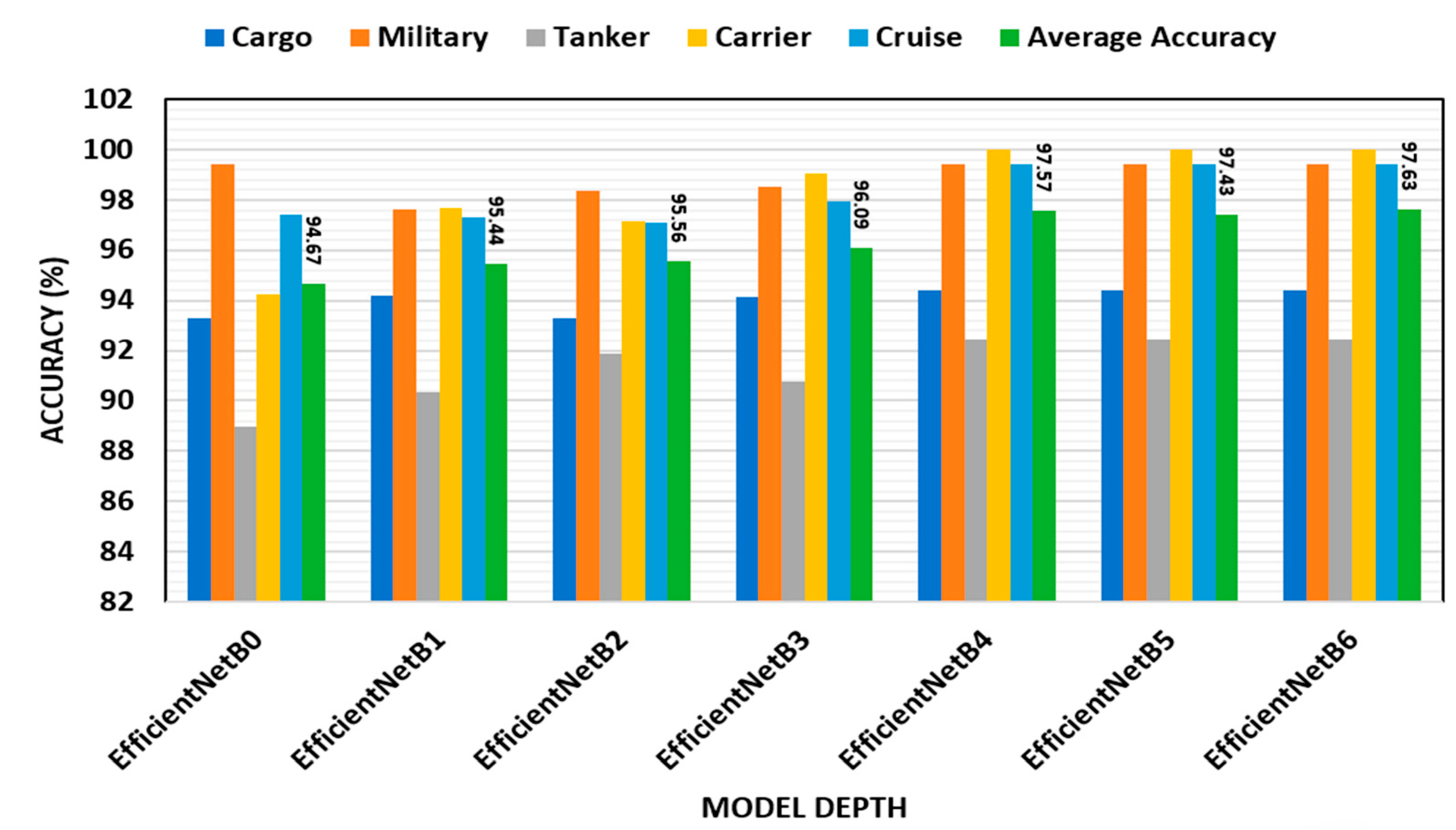
Figure 5 demonstrates how the accuracy of the public ship dataset’s performance was impacted by the network depth. It was found that raising the network depth improved the EfficientNetB model’s performance. As a consequence, EfficientNetB enhanced performance with fewer depth layers in terms of accuracy for the Game of Deep Learning Ship dataset types (i.e., EfficientNetB0 to EfficientNetB6). Since the average accuracy is almost constant after EfficientNetB2, with the parameters being highly increased, EfficientNetB2 is chosen for the modified and ensemble learning stages.
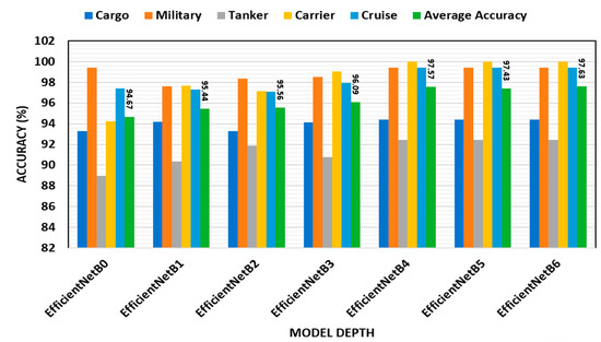
Figure 5.
Different depth layers accuracy performance for ship classification dataset.
4.4.2. Modified CNN Model
As was discussed in the preceding section, the proposed EfficientNetB2 structure is selected to boost the network’s performance. Three additional blocks are added, with each block consisting of a fully connected (FC) layer. Following this layer, a ReLU layer was added to learn the new properties of our training dataset. This layer was followed by dropout layers. The modified EfficientNetB2 architecture is illustrated in Figure 6. With the help of a publicly available ship dataset and a number of different permutations of the vectors of fully linked layers in the proposed classifying block, an efficient EfficientNetB2 model was investigated. The goals of this research were to make the network more stable and find the fully connected layers with the best feature extraction vector.
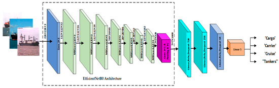
Figure 6.
Modified EfficientNetB2 Architecture.
However, in order to accomplish transfer learning, the features that were collected from earlier layers were used to propose the classification block, obtaining the ideal weight and distortion from the input dataset. The proposed classification method was trained and validated using the same learning and momentum parameters. The suggested network of two fully linked (connected) layers, with higher functional vectors, had a much higher precision compared to other fully connected layers, with lower functional vectors. The first layer, which was totally related to 1408 characteristics, was located beneath the classifying block. At the same time, the classifying network block received the introduction of the highly functioning, fully connected layers. The examination of our network at various depth layers came next. Table 4 displays the accuracy of each layer to demonstrate the network’s performance.
Table 4.
EfficientNetB2Different feature vectors performance.
Several learning rates were acquired in order to build a classification network with a total accuracy of 97.75%. By using the modified EfficientNetB2architecture, adding a classification block with three fully connected layers, followed by a ReLU layer and dropout layer, and testing it on a dataset from the Game of Deep Learning Ship datset, our suggested method outperformed earlier results. Table 4 lists the performance indicators.
4.4.3. Ensemble Learning (EL)
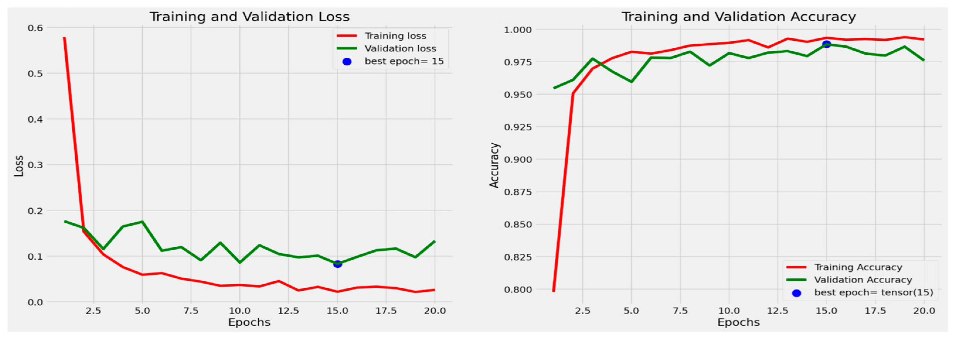
The performance of the final modified system is obtained using ensemble learning (EL). The EL model performance is illustrated in Figure 7 and Figure 8. Training and validation loss and accuracy for the game ship classification dataset are shown in Figure 7. The highest accuracy achieved in the game ship classification dataset is marked by the blue dot (98.38%).
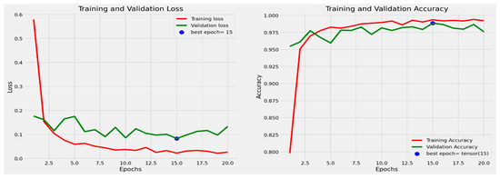
Figure 7.
Training and validation loss and Accuracy for game ship classification dataset.
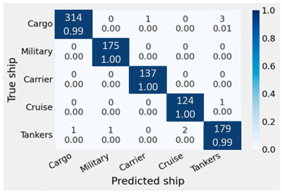
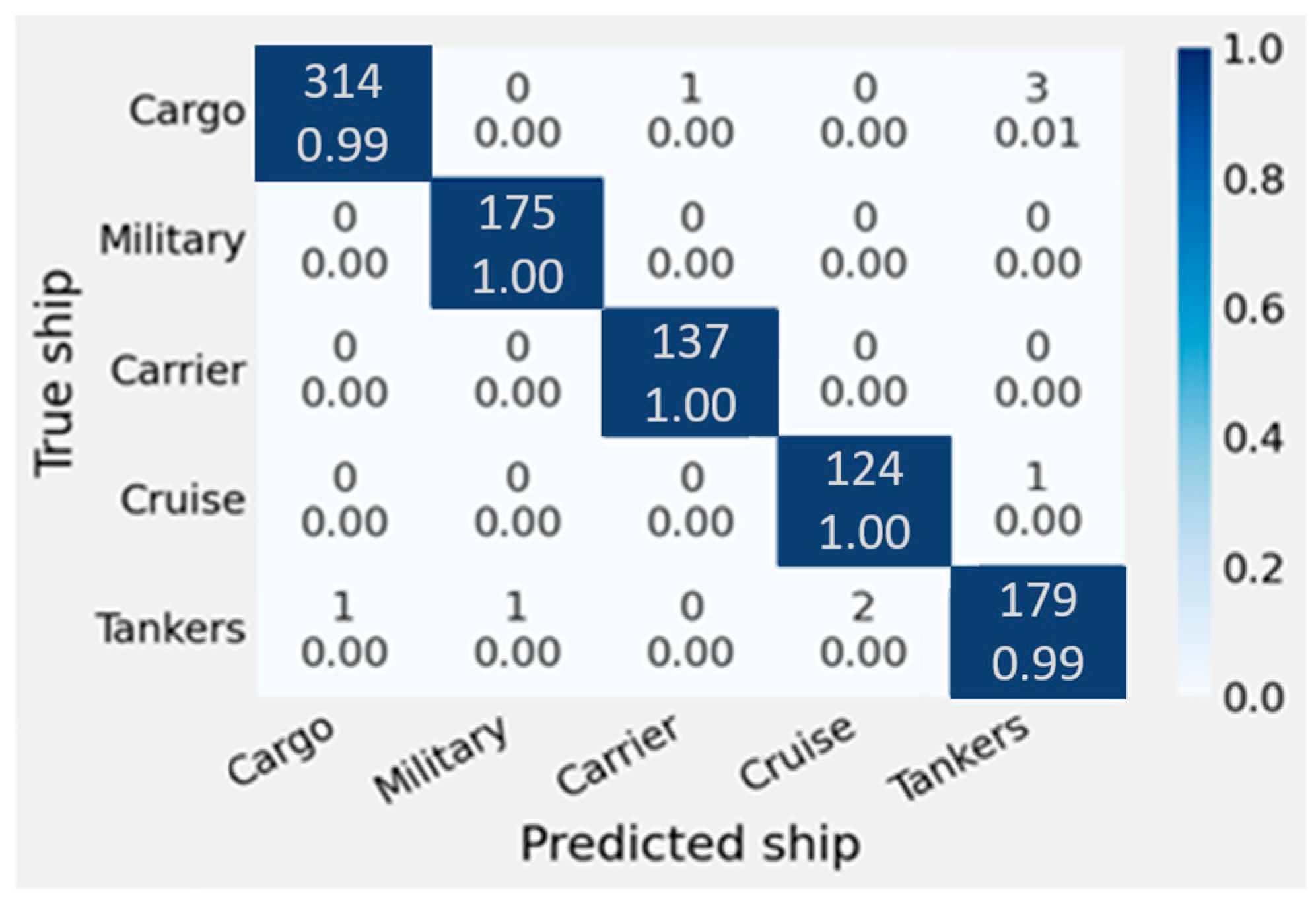
Figure 8.
Confusion matrix for game ship classification dataset.
To indicate the accuracy of different class ship classifications, the confusion matrix for the game ship classification dataset is shown in Figure 8. The accuracy values demonstrate the integration of the modified model with the optimization of hyper-parameters, then the ensemble learning for the best three models with confidence averaging, which gives higher accuracy than concatenation ensemble learning.
The EfficientNetB2 precision performance matrices may be seen in Table 5. The accuracy of the classification system reached a total of 98.34% overall. The cargo and tanker classes scored the lowest precision, coming in at 97.86% and 95.75%, respectively, in their results. The military, aircraft carriers, and cruise ships were correctly classified at a rate of more than 98%. The results indicate that it performed well in terms of specificity and that it worked well overall.
Table 5.
Evaluation metrics for the Game of Deep Learning Ship dataset.
In Table 6, the results for the final modified model accuracy after optimization, concatenation and confidence averaging ensemble learning (EL) are presented. The three best performance models are combined using the two ensemble learning methods. Confidence averaging shows better performance.
Table 6.
Evaluation metrics using different ensemble learning methods.
4.5. MARVEL Dataset Experimental Result
For generalizability, the classification experiment analysis was applied to another publicly available dataset, MARVEL [7]. The selected dataset is divided into 26 different common ship categories. This dataset could better distinguish the classification capabilities of various neural networks for inland ships, thus reflecting the detection performance when various classification networks were adjusted as the backbone network. This was conducted to ensure the generalizability of our proposed network. Cargo, military, cruise, carrier, and tanker were the five categories chosen. A total of 540 photos from each category was randomly chosen to serve as the test images for the proposed classification scheme.
In order to accurately evaluate the capabilities of our system, we relied solely on the test images; the network was not retrained. Table 7 presents the classification precision achieved with this MARVEL dataset for our perusal.
Table 7.
Classification performance for the MARVEL dataset.
A better result was achieved, even though a different dataset was employed. The proposed ship classification approach performed well even when applied to a new dataset.
To indicate the accuracy of different class ship classification, the confusion matrix for MARVEL ship classification dataset is shown in Figure 9. The accuracy values indicate the higher accuracy achieved with the integration of modified model and the optimization of hyper-parameters, then the ensemble learning for the best three models with confidence averaging.
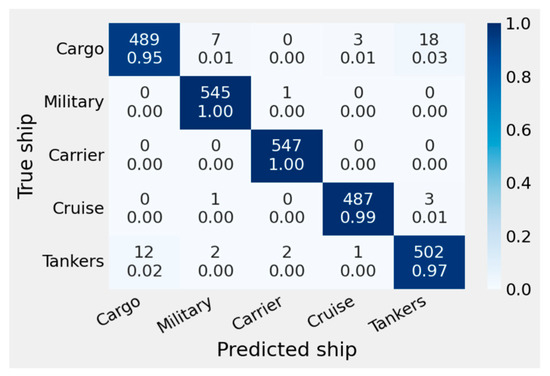
Figure 9.
Confusion matrix for MARVEL dataset.
Table 7 shows the results of testing our proposed ensemble transfer learning ship classification system with the MARVEL public dataset [7]. Retraining is not used to measure the generalization performance. Table 7 shows that the suggested model outperforms a different dataset. Tanker Acc is 94.61%, whereas carrier Acc is 100%. Military Acc is 98.42%, Cargo Acc is 97.65% and Cruise Acc 94.5%. The total performance statistics show an overall 97.04 Acc, 96.1 Pre, 95.92% Rec, and 96.55% F1. The study’s findings indicate a strong classification performance using a different dataset, proving the model’s generalization capacity.
4.6. Comparison to Related Works
This section provides a contrast and comparison analysis of the proposed algorithm with several other existing approaches. Most studies on ship classification rely on a public dataset. A challenge remains, though, in standardizing the diverse research approaches that have been taken. Table 8 compares the overall performance of our inquiry with the most recent methodologies mentioned in the published literature. A system for classifying ships based on SAR photos and in situ data was developed by Wang et al. [37]. This was found by using a backscattering-based categorization and the shape of the ship. It was 82% accurate.
Table 8.
Comparison between state-of-the-art algorithms.
A DL classification network based on CNN architecture with gnostic field technology was presented by Zhang et al. [8]. They used 0.2 for the gnostic field output and 0.8 for the CNN output. The system achieves an accuracy of 87.40%. Three types of ships were classified by Jiang et al. [38] based on their dispersion qualities. Their assignment was performed with a boat-length ratio of 83.33%.
Gundogdu et al. [9] introduced an ML method; an SVM-classified CNN model is utilized to extract deep features. Sheng et al. [39] used a raw underwater audio stream to identify and classify ships in another study that was motivated by the auditory CNN model. The classification accuracy rating for five ship classes in the experiments came to 79.2%. The CNN-inspired auditory approach used by Shen et al. [39] generated extensive analysis, but the five-class classification template produced subpar results. The Inception V3 network was employed with the transfer learning technique by Leclerc et al. [22].
Several learning rates were acquired to build an efficient classification network with higher accuracy. Using the modified EfficientNetB2 architecture, and adding a classification block with three fully connected layers, was chosen as the best of the three models for ensemble learning. Previous research and testing on a dataset from the standard ship datasets showed that our method worked better. Table 8 lists the performance indicators for the ship dataset [40].
We compared the performance of our ensemble transfer learning with state-of-the-art ship classification methods for the MARVEL dataset. The metric rendition of the most modern techniques for each class of ship is shown in Table 9. Despite Wang et al. [37] claiming the lowest accuracy in the tanker and cargo classes, Jiang et al. [38] demonstrated the most insufficient accuracy in the carrier class. The armed forces and cruise ships had no classes. Acceptable classification accuracy was attained by Ucar et al. [25] when compared to our suggested technique for the military and cruise ship classes. Still, poor classification accuracy was achieved compared to our suggested methodology for the other categories of ships. As can be seen from the results of the comparison, our proposed strategy outperformed the others.
Table 9.
Classification result of MARVEL with state-of-the-art algorithms.
5. Conclusions
In this paper, we developed an enhanced model architecture for classification that is based on transfer learning and ensemble learning to classify ships using optimized CNN models for inland waterways. As a result, the classification model for classifying ships performed better. The model is trained with the public dataset “Game of Deep Learning”. The dataset includes five classes: cargo, military, carrier, cruise, and tanker ships. Eight pre-trained models are utilized for training. The EfficientNetB0 model records the best accuracy. First, the best model architecture was enhanced by optimizing the model hyperparameters. PSO is applied for optimizing the model parameters that affect the performance. The model architecture is then modified to improve classification and inter-class performance. The three most effective models were chosen for further development based on ensemble learning. An augmentation-based data transformation technique is also suggested to convert ship image data for the CNN models.
With a success rate of 98.38%, the ensemble learning model outperformed the competition. Specifically, we enhanced the system by adding a new classification block consisting of three fully linked layers followed by ReLU and a dropout layer. The proposed technique has a higher success rate than the best existing algorithms.
Our ship classification system was used on the publicly available MARVEL dataset to gauge how effectively the suggested classification method can be generalized to other larger datasets. A degree of accuracy of 96.36% was found in this experiment, proving that the proposed method is effective. Finally, the system was compared to other existing algorithms for categorizing various ship classes in inland waterways, and our suggested solution outperformed the others. In further studies, the proposed method will be improved so that ships in different weather conditions may be classified for the modern vessel classification system that requires fast processing and small data samples. Compelling image preprocessing will look at how well the classification works for noisy and low-contrast images.
Author Contributions
Conceptualization, methodology and writing—original draft, M.H.S.; methodology, validation and supervision, Y.L.; formal analysis and review, Z.L.; review and editing, A.M.A. All authors have read and agreed to the published version of the manuscript.
Funding
This research received no external funding.
Institutional Review Board Statement
Not applicable.
Informed Consent Statement
Not applicable.
Data Availability Statement
Data is available in the manuscript.
Conflicts of Interest
The authors declare no conflict of interest.
References
- Du, Q.; Zhang, Y.; Yang, X.; Liu, W. Ship target classification based on Hu invariant moments and ART for maritime video surveillance. In Proceedings of the 2017 4th International Conference on Transportation Information and Safety (ICTIS), Banff, AB, Canada, 8–10 August 2017; pp. 414–419. [Google Scholar] [CrossRef]
- Gallego, A.-J.; Pertusa, A.; Gil, P. Automatic Ship Classification from Optical Aerial Images with Convolutional Neural Networks. Remote Sens. 2018, 10, 511. [Google Scholar] [CrossRef]
- Grinblat, L.; Uzal, L.C.; Larese, M.G.; Granitto, P.M. Deep learning for plant identification using vein morphological patterns. Comput. Electron. Agric. 2016, 127, 418–424. [Google Scholar] [CrossRef]
- Chouhan, S.S.; Kaul, A.; Singh, U.P. Image Segmentation Using Computational Intelligence Techniques: Review. Arch. Comput. Methods Eng. 2019, 26, 533–596. [Google Scholar] [CrossRef]
- Chollet, F. Xception: Deep Learning with Depthwise Separable Convolutions. In Proceedings of the 2017 IEEE Conference on Computer Vision and Pattern Recognition (CVPR), Honolulu, HI, USA, 21–26 July 2017; pp. 1800–1807. [Google Scholar]
- Wang, Y.; Yao, Q.; Kwok, J.T.; Ni, L.M. Generalizing from a Few Examples. ACM Comput. Surv. 2020, 53, 63. [Google Scholar] [CrossRef]
- Moosbauer, S.; Konig, D.; Jakel, J.; Teutsch, M. A benchmark for deep learning based object detection in maritime environments. In Proceedings of the 2019 IEEE/CVF Conference on Computer Vision and Pattern Recognition Workshops (CVPRW), Long Beach, CA, USA, 16–17 June 2019; pp. 916–925. [Google Scholar]
- Prasad, D.K.; Rajan, D.; Rachmawati, L.; Rajabally, E.; Quek, C. Video Processing From Electro-Optical Sensors for Object Detection and Tracking in a Maritime Environment: A Survey. IEEE Trans. Intell. Transp. Syst. 2017, 18, 1993–2016. [Google Scholar] [CrossRef]
- Gundogdu, E.; Solmaz, B.; Yücesoy, V.; Koç, A. MARVEL: A Large-Scale Image Dataset for Maritime Vessels. In Computer Vision—ACCV 2016. ACCV 2016; Lecture Notes in Computer Science; Springer: Cham, Switerland, 2016; Volume 10115, pp. 165–180. [Google Scholar] [CrossRef]
- Zhang, M.M.; Choi, J.; Daniilidis, K.; Wolf, M.T.; Kanan, C. VAIS: A dataset for recognizing maritime imagery in the visible and infrared spectrums. In Proceedings of the IEEE Computer Society Conference on Computer Vision and Pattern Recognition Workshops, Boston, MA, USA, 7–12 June 2015; pp. 10–16. [Google Scholar]
- Buda, M.; Maki, A.; Mazurowski, M.A. A systematic study of the class imbalance problem in convolutional neural networks. Neural Netw. 2018, 106, 249–259. [Google Scholar] [CrossRef] [PubMed]
- Dao-Duc, C.; Xiaohui, H.; Morère, O. Maritime vessel images classification using deep convolutional neural networks. In Proceedings of the Sixth International Symposium on Information and Communication Technology, Hue, Vietnam, 3–4 December 2015; pp. 276–281. [Google Scholar] [CrossRef]
- Rawat, W.; Wang, Z. Deep convolutional neural networks for image classification: A comprehensive review. Neural Comput. 2017, 29, 2352–2449. [Google Scholar] [CrossRef]
- Yosinski, J.; Clune, J.; Bengio, Y.; Lipson, H. How transferable are features in deep neural networks? arXiv 2014, arXiv:1411.1792. [Google Scholar]
- Oquab, M.; Bottou, L.; Laptev, I.; Sivic, J. Learning and transferring mid-level image representations using convolutional neural networks. In Proceedings of the IEEE Conference on Computer Vision and Pattern Recognition, Columbus, OH, USA, 23–28 June 2014. [Google Scholar]
- Iandola, F.N.; Han, S.; Moskewicz, M.W.; Ashraf, K.; Dally, W.J.; Keutzer, K. SqueezeNet: AlexNet-level accuracy with 50× fewer parameters and <0.5 MB model size. arXiv 2016, arXiv:1602.07360. [Google Scholar] [CrossRef]
- Shi, Q.; Li, W.; Zhang, F.; Hu, W.; Sun, X.; Gao, L. Deep CNN with Multi-Scale Rotation Invariance Features for Ship Classification. IEEE Access 2018, 6, 38656–38668. [Google Scholar] [CrossRef]
- Tan, M.; Le, Q.V. EfficientNet: Rethinking Model Scaling for Convolutional Neural Networks. In Proceedings of the 36th International Conference on Machine Learning, Long Beach, CA, USA, 9–15 June 2019; pp. 10691–10700. [Google Scholar]
- Yang, L.; Shami, A. On hyperparameter optimization of machine learning algorithms: Theory and practice. Neurocomputing 2020, 415, 295–316. [Google Scholar] [CrossRef]
- Bloisi, D.D.; Iocchi, L.; Pennisi, A.; Tombolini, L. ARGOS-Venice Boat Classification. In Proceedings of the 2015 12th IEEE International Conference on Advanced Video and Signal Based Surveillance (AVSS), Karlsruhe, Germany, 25–28 August 2015. [Google Scholar] [CrossRef]
- Khellal, A.; Ma, H.; Fei, Q. Convolutional Neural Network Based on Extreme Learning Machine for Maritime Ships Recognition in Infrared Images. Sensors 2018, 18, 1490. [Google Scholar] [CrossRef] [PubMed]
- Leclerc, M.; Tharmarasa, R.; Florea, M.C.; Boury-Brisset, A.C.; Kirubarajan, T.; Duclos-Hindié, N. Ship Classification Using Deep Learning Techniques for Maritime Target Tracking. In Proceedings of the 2018 21st International Conference on Information Fusion, Cambridge, UK, 10–13 July 2018; pp. 737–744. [Google Scholar] [CrossRef]
- Yao, B.; Yang, J.; Ren, Y.; Zhang, Q.; Guo, Z. Research and comparison of ship classification algorithms based on variant CNNs. In Proceedings of the 2019 IEEE 3rd Information Technology, Networking, Electronic and Automation Control Conference (ITNEC), Chengdu, China, 15–17 March 2019; pp. 918–922. [Google Scholar] [CrossRef]
- Shi, Q.; Li, W.; Tao, R.; Sun, X.; Gao, L. Ship Classification Based on Multifeature Ensemble with Convolutional Neural Network. Remote Sens. 2019, 11, 419. [Google Scholar] [CrossRef]
- Ucar, F.; Korkmaz, D. A novel ship classification network with cascade deep features for line-of-sight sea data. Mach. Vis. Appl. 2021, 32, 73. [Google Scholar] [CrossRef]
- Leonidas, L.A.; Jie, Y. Ship Classification Based on Improved Convolutional Neural Network Architecture for Intelligent Transport Systems. Information 2021, 12, 302. [Google Scholar] [CrossRef]
- Karen, S.; Andrew, Z. Very deep convolutional networks for large-scale image recognition. In Proceedings of the 3rd International Conference on Learning Representations (ICLR 2015), San Diego, CA, USA, 7–9 May 2015. Conference Track Proceedings. [Google Scholar]
- He, K.; Zhang, X.; Ren, S.; Sun, J. Deep residual learning for image recognition. In Proceedings of the IEEE Computer Society Conference on Computer Vision and Pattern Recognition, Las Vegas, NV, USA, 27–30 June 2016. [Google Scholar]
- Szegedy, C.; Vanhoucke, V.; Ioffe, S.; Shlens, J.; Wojna, Z. Rethinking the Inception Architecture for Computer Vision. In Proceedings of the IEEE Conference on Computer Vision and Pattern Recognition (CVPR), Las Vegas, NV, USA, 27–30 June 2016; pp. 2818–2826. [Google Scholar] [CrossRef]
- Szegedy, C.; Ioffe, S.; Vanhoucke, V.; Alemi, A.A. Inception-v4, Inception-ResNet and the Impact of Residual Connections on Learning. In Proceedings of the Thirty-First AAAI Conference on Artificial Intelligence, San Francisco, CA, USA, 4–9 February 2017; pp. 4278–4284. [Google Scholar] [CrossRef]
- Huang, G.; Liu, Z.; van der Maaten, L.; Weinberger, K.Q. Densely Connected Convolutional Networks. In Proceedings of the IEEE Conference on Computer Vision and Pattern Recognition (CVPR), Honolulu, HI, USA, 21–26 July 2017; pp. 2261–2269. [Google Scholar]
- Howard, A.G.; Zhu, M.; Chen, B.; Kalenichenko, D.; Wang, W.; Weyand, T.; Andreetto, M.; Adam, H. MobileNets: Efficient Convolutional Neural Networks for Mobile Vision Applications. arXiv 2017, arXiv:1704.04861. [Google Scholar] [CrossRef]
- Sandler, M.; Howard, A.; Zhu, M.; Zhmoginov, A.; Chen, L.C. MobileNetV2: Inverted Residuals and Linear Bottlenecks. In Proceedings of the IEEE/CVF Conference on Computer Vision and Pattern Recognition (CVPR), Salt Lake City, UT, USA, 18–23 June 2018; pp. 4510–4520. [Google Scholar] [CrossRef]
- Large, J.; Lines, J.; Bagnall, A. A probabilistic classifier ensemble weighting scheme based on cross-validated accuracy estimates. Data Min. Knowl. Discov. 2019, 33, 1674–1709. [Google Scholar] [CrossRef]
- Rahimzadeh, M.; Attar, A. A modified deep convolutional neural network for detecting COVID-19 and pneumonia from chest X-ray images based on the concatenation of Xception and ResNet50V2. Inform. Med. Unlocked 2020, 19, 100360. [Google Scholar] [CrossRef]
- Game of Deep Learning: Ship Datasets|Kaggle. Available online: https://www.kaggle.com/datasets/arpitjain007/game-of-deep-learning-ship-datasets (accessed on 23 November 2022).
- Wang, C.; Zhang, H.; Wu, F.; Jiang, S.; Zhang, B.; Tang, Y. A novel hierarchical ship classifier for COSMO-SkyMed SAR data. IEEE Geosci. Remote Sens. Lett. 2014, 11, 484–488. [Google Scholar] [CrossRef]
- Jiang, M.; Yang, X.; Dong, Z.; Fang, S.; Meng, J. Ship classification based on superstructure scattering features in SAR images. IEEE Geosci. Remote Sens. Lett. 2016, 13, 616–620. [Google Scholar] [CrossRef]
- Shen, S.; Yang, H.; Li, J.; Xu, G.; Sheng, M. Auditory Inspired Convolutional Neural Networks for Ship Type Classification with Raw Hydrophone Data. Entropy 2018, 20, 990. [Google Scholar] [CrossRef] [PubMed]
- García, J.; Concha, O.P.; Molina, J.M.; De Miguel, G. Trajectory classification based on machine-learning techniques over tracking data. In Proceedings of the 2006 9th International Conference on Information Fusion, Florence, Italy, 10–13 July 2006. [Google Scholar] [CrossRef]


Disclaimer/Publisher’s Note: The statements, opinions and data contained in all publications are solely those of the individual author(s) and contributor(s) and not of MDPI and/or the editor(s). MDPI and/or the editor(s) disclaim responsibility for any injury to people or property resulting from any ideas, methods, instructions or products referred to in the content. |
© 2023 by the authors. Licensee MDPI, Basel, Switzerland. This article is an open access article distributed under the terms and conditions of the Creative Commons Attribution (CC BY) license (https://creativecommons.org/licenses/by/4.0/).