Abstract
Synchronisation of a voice recording with the corresponding text is a common task in speech and music processing, and is used in many practical applications (automatic subtitling, audio indexing, etc.). A common approach derives a mid-level feature from the audio and finds its alignment to the text by means of maximizing a similarity measure via Dynamic Time Warping (DTW). Recently, a Connectionist Temporal Classification (CTC) approach was proposed that directly emits character probabilities and uses those to find the optimal text-to-voice alignment. While this method yields promising results, the memory complexity of the optimal alignment search remains quadratic in input lengths, limiting its application to relatively short recordings. In this work, we describe how recent improvements brought to the textbook DTW algorithm can be adapted to the CTC context to achieve linear memory complexity. We then detail our overall solution and demonstrate that it can align text to several hours of audio with a mean alignment error of 50 ms for speech, and 120 ms for singing voice, which corresponds to a median alignment error that is below 50 ms for both voice types. Finally, we evaluate its robustness to transcription errors and different languages.
1. Introduction
The text-to-voice alignment problem originated in the late 1970s. Historically, it emerged in the speech recognition community from the need to automatically segment and label voice recordings to build large corpora of paired audio and text. It has found since then several other applications for the general public, e.g., text-based audio indexing, automatic closed captioning, or karaoke. A wealth of different implementations have been proposed over the last few decades to address this problem. However, they all follow the same general two-step principle: (1) a timestamped encoding of the audio voice recording, and (2) a forced alignment mapping this timing information to the ground-truth text, as depicted on Figure 1.
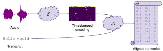
Figure 1.
Audio-to-text forced alignment principle: timestamped encoding of audio inputs followed by forced alignment mapping timestamps to text.
The sequence alignment problem is not unique to speech processing. Several research communities were confronted with the same question and have rediscovered simultaneously and independently a similar algorithm to find the optimal correspondence between two sequences and to estimate their homology, e.g., in telecommunications [1], bioinformatics [2], or speech processing [3,4]. As this algorithm relies on dynamic programming (DP), it was named Dynamic Time Warping (DTW) by the speech recognition community [5]. Besides text-to-voice synchronization, DTW usage then spread to numerous other applications involving audio sequence alignment, such as melody search [6], score following [7], audio matching [8], beat tracking [9], or version identification [10], among many others.
The forced alignment step of text-to-voice synchronization has therefore generally relied on the original DTW algorithm or one of its variants. The encoding step , on the contrary, has been implemented with multiple approaches over the last decades. In the 1980s, pioneering works were limited to short utterance synchronization, extracting signal processing-based parameters from the audio and using some domain knowledge-based rules to force-align these parameters to the ground-truth phoneme sequence [11,12].
In the 1990s, the encoding step was leveraging the Automatic Speech Recognition (ASR) systems available at that time. These ASR systems were generally relying on Hidden Markov Models (HMMs) to model the sequential structure of the speech. The HMM emission probabilities were typically represented by mixtures of Gaussians (GMMs) modeling some spectral observations derived from the audio, e.g., Mel-frequency cepstrum (MFC), whereas the HMM hidden states represented the corresponding phoneme or grapheme time series [13,14]. These HMM-based systems were further improved in the 2000s to specifically address the need to synchronize very long audio recordings [15,16,17,18,19,20,21,22]. Their usage was also recently extended to lyrics and singing voice synchronization [23].
The success of Deep Neural Networks (DNNs) in many other fields during the 2010s motivated their progressive adoption in ASR systems. DNNs were first introduced in hybrid DNN–HMM architectures to address the limitations of GMMs in modeling high-dimensional data [24]. DNNs were then implemented in end-to-end architectures to replace HMMs and to overcome the limitations induced by HMM-underlying Markov assumptions [25]. Along with their ability to model the long-term dependencies in speech, DNN-based end-to-end systems also greatly simplified the processing pipeline of the earlier HMM-based approaches, which required complex expert knowledge [26].
Given the proximity between voice recognition and voice alignment problems, the success of DNN reported in the ASR literature motivated their usage for voice-to-text synchronization. Early attempts in that direction considered the alignment task as a frame-wise classification problem and aimed at predicting the correct symbol at each time step [27,28]. However, the large amounts of paired audio and precisely time-aligned text required to train these architectures are tedious to collect. Other approaches that could be trained with more widespread data, such as paired audio and text without precise timing information, were therefore investigated.
It was, for instance, recently proposed to consider the alignment task as an auxiliary objective for the source separation problem and to learn the optimal alignment maximising the separation quality [29,30]. It was also proposed to leverage recent advances made by ASR systems based on Connectionist Temporal Classification (CTC). The CTC loss was initially introduced to train Recurrent Neural Networks (RNNs) on unsegmented data [31] and became ubiquitous in the speech recognition literature [32,33,34,35,36,37]. Given some audio inputs, a CTC-based network is trained to output a posteriorgram which predicts at each time frame the discrete probability distribution over a lexicon of labels, typically graphemes. While the temporal information contained in the posteriorgram is usually dropped for speech recognition as such, it can be decoded with a DTW-alike algorithm to obtain a forced-alignment of the ground-truth text [38,39].
The possibility offered by CTC-based architectures to transcribe the audio waveform directly into graphemes in an end-to-end fashion renders this approach particularly appealing for text to spoken or singing voice synchronization. However, the CTC forced-alignment step, similar to that of DTW, requires the computation of an alignment path that scales quadratically in the sequence lengths, both in time and space. This rapidly becomes prohibitive for long audio alignment, a common use case for modern research and consumer applications. Many optimizations of the DTW algorithm have been proposed in the past to reduce its complexity, generally at the cost of some approximations. Recently, however, an exact reformulation of the DTW algorithm scaling linearly in memory was released [40].
In this work, we address the problem of text-to-voice alignment for very long audio recordings, which is a growing need in the academic field, e.g., to automatically synchronize large corpora of paired voice and text for downstream tasks, such as voice synthesis. Our approach involves CTC-based modeling and an adaptation of the linear memory DTW to the CTC context. It offers several advantages: our end-to-end architecture avoids the complexity of legacy HMM-based solutions, and our linear memory CTC decoding avoids the necessity to segment long audio into imprecise shorter chunks before synchronization.
Our contributions are: (1) we introduce an adaptation of the linear memory DTW to to the CTC context for step , extending the use of CTC-based algorithms for the alignment of very long audio recordings; (2) we describe a CTC-based fully-convolutional neural architecture agnostic to audio duration for step ; (3) we demonstrate that our system is able to synchronize several hours of audio with the corresponding text, yielding a mean absolute alignment error of 50 ms for speech and 120 ms for the singing voice, which corresponds to a median alignment error that is below 50 ms for both voice types; (4) we illustrate its robustness against deteriorated transcripts; (5) we demonstrate that, albeit being trained solely on unsegmented audio and text in English, it achieves similar performances for many other languages; (6) we compare it to the state-of-the art systems and demonstrate that our simple end-to-end approach rivals much more complex systems on publicly available datasets.
The rest of this paper is structured as follows. In Section 2, we briefly describe the recent research that inspired our present work. In Section 3, we first provide a short reminder of the textbook DTW algorithm and its linear memory reformulation, and then describe how it can be adapted to a linear memory CTC forced-alignment algorithm. We provide the details of our experiments and describe our results in Section 4. We conclude with our future perspectives.
2. Related Works
In this section, we summarize the recent advances that inspired our present work, i.e., the use of a neural CTC acoustic model for the audio timestamped encoding step , and an optimized DTW for the alignment step .
2.1. CTC-Based Modeling for the Encoding Step
In our applicative context, the timestamped encoding can be implemented as the output of a CTC-trained neural network trained on audio directly, which represents the per-frame character emission probabilities—referred to as posteriorgram.
To the best of our knowledge, Stoller et al. [38] were the first to exploit this strategy when they explicitly leveraged the time dimension of CTC posteriorgrams to align the lyrics and singing voice with background music. By extracting multi-scale representations from raw audio samples with a Wav-U-Net architecture [41], trained on a 40k+ song proprietary dataset, the authors proved the feasibility of aligning polyphonic music with an end-to-end CTC acoustic prediction framework, and demonstrated the interest of this approach for text-to-voice alignment in general. For instance, Kurzinger et al. [39] used a CTC-based neural network originally trained for ASR purposes to segment, at the sentence level, a large corpus of German speech recordings, and demonstrated that this approach clearly outperformed HMM-based legacy methods in terms of alignment precision.
In the same vein, and following the success of their CTC-based model in other tasks [42,43], Vaglio et al. [44] demonstrated that a plain Convolutional Recurrent Neural Network (CRNN) could also yield promising performances. Trained with the publicly available data contained in DALI [45], the authors tackled the issue of voice alignment in a multilingual context, even for language with almost no training data.
More recently, Teytaut et al. studied the impact of adding additional constraints to the CTC in order to improve the accuracy of the posteriorgrams. By combining the CTC loss with a spectral reconstruction cost in an encoder–decoder architecture [46], better synchronization precision was achieved for clean recordings featuring solo speaking and a singing voice. This precision at the phonetic level could be used to analyze the temporal aspects involved in the production strategies of vocal attitudes in expressive speech [47,48]. Further works have proposed other types of regularizations enforcing audio-text monotony and structural similarity [49], but did not specifically focus on long audio alignments, as opposed to our present work.
2.2. Optimized DTW for the Alignment Step
When considering the alignment step , we note that a majority of the approaches discussed so far rely on Dynamic Time Warping or one of its variants. We briefly introduce the research dedicated to its optimization.
The textbook DTW algorithm to align two sequences and implies a pairwise sequence element comparison (forward pass) and traces back the optimal alignment path minimizing the total alignment cost (backward pass). The forward pass computing the pairwise distance matrix has a quadratic complexity in in time and space, which quickly becomes problematic for many use cases, such as a similar sequence search in large corpora or long sequence alignment.
In the context of sequence indexing, a common solution to speed up the computation of the DTW alignment cost was to seek for a cheap-to-compute lower bounding function to prune unpromising candidates [50,51,52]. This approach proved its efficiency to mine trillions of sequences [53], but discards the concept of the alignment path that is required to address the alignment problem, per se.
A classical approach to speed up the computation of the alignment path—and not only the alignment cost—is to avoid an exhaustive search among all possible paths, by restricting the exploration within some boundaries, e.g., a band or a parallelogram around the diagonal of the pairwise distance matrix [5,54]. This is generally an effective solution, as extreme warping between sequences is often unlikely, but yields an incorrect result if the actual alignment lies outside the explored area.
Several global adaptive constraints have thus been proposed to restrict the exploration area, such as multi-scale alignments where an optimal path is found at a coarse level and is gradually refined at increasingly accurate resolutions [55,56,57], or segment-level alignments that serve to further refine frame-level alignments [58]. Further improvements have been proposed with local adaptive constraints to restrict the exploration more precisely to the vicinity of the optimal path, for instance by gradually expanding the current optimal path via a local greedy search [59,60], or by searching and concatenating overlapping block sub-alignments [61]. Early abandoning is another adaptive strategy used to prune unpromising alignment paths when the alignment cost exceeds some threshold [62,63]. These constrained algorithms generally achieve a linear space complexity at the cost of only providing an approximate solution.
On the contrary, Tralie and Dempsey [40] recently proposed a clever reformulation of the textbook DTW that is both exact and has linear space complexity. In the next section, we will detail this algorithm and explain how our own algorithm adapts these ideas to the CTC context.
3. Method
In this section, we first present a succinct reminder about the textbook DTW algorithm and its linear memory version, which will serve as a basis for the rest of the paper. We then present the Connectionist Temporal Classification (CTC) concepts that are important for our purpose, and draw a parallel with the textbook DTW algorithm. We finally introduce our contributions: (1) we describe a linear memory version of the CTC alignment algorithm that can be used for the very long audio-text forced alignment step , and (2) we describe the neural network that we used for the encoding step .
3.1. The Textbook DTW Alignment Algorithm
We present here a succinct reminder about the textbook DTW algorithm [3,4,5] to introduce notations and concepts used throughout this paper.
3.1.1. Definitions
Let and denote two feature spaces, and let and denote the sets of all sequences over and , respectively. Let be a sequence, and let denote its length, and be the subsequence containing its n first elements.
A notion of the correspondence between the ordered elements of two sequences and can be depicted by a sequence of the ordered tuples of and indices:
is called a pathway [2], a warping function [5], a warping or alignment path, or simply a path if it also satisfies some additional constraints:
- Boundaries: starts and ends at the beginning and end of each sequence, i.e.,:
- Monotonicity: does not go backward, i.e.,:The Figure 2 illustrates these constraints:
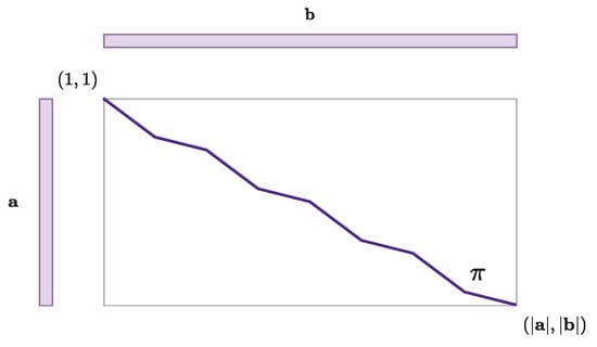 Figure 2. A monotonically evolving alignment path between two sequences and .
The transitions between successive points on path are typically limited to a set of permitted gaps. For instance, the textbook alignment algorithm imposes a maximum shift of one element on both axis, i.e.,:
The Figure 3 illustrates the textbook-permitted transitions.
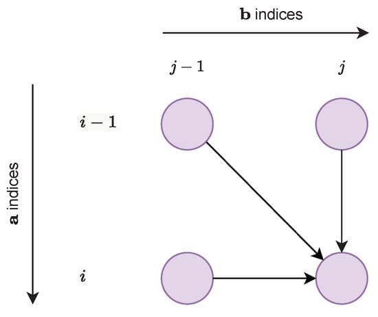
Figure 3.
Textbook DTW alignment path-permitted transitions.
Let denote a similarity measure between elements of and (the textbook DTW uses a cost measure, but we use here a similarity measure to draw the parallel with the CTC alignment below). Aligning the sequences and consists in finding the path that maximises the sum of the similarity measures of its elements:
is called the optimal path, and is called the optimal alignment measure.
3.1.2. * Computation via Dynamic Programming
Solving Equation (4) directly is usually intractable, as there are too many possible paths between the two sequences. It is, however, possible to compute it indirectly, noticing that the optimal similarity measure between two sequences can be obtained recursively, considering the similarity measure between the two sequence prefixes.
As depicted on Figure 3, if the optimal path between two sequences passes through the point , it necessarily passes through one of the points , , or . It is thus enough to know the optimal similarity measure on these 3 predecessors to deduce the optimal similarity measure on the point .
Let denote the optimal alignment similarity between the prefix and the prefix , and assume that , , and are already known. Given the permitted path transitions depicted on Figure 3, it is straightforward to see that:
The initialisation step is given by:
The optimal global alignment similarity can then be computed recursively using Equations (6) and (7), accumulating at each step the similarity measure of the best predecessor optimal path (forward pass). The optimal path can then be traced back using the sequence of optimal transitions retained in the forward pass (backward pass).
The computation of the matrix during the forward pass has a computational and memory complexity that scales quadratically in . This rapidly becomes problematic for long sequences.
3.2. Linear Memory DTW Algorithm
Tralie and Dempsey [40] proposed an algorithm to compute and exactly, but with a space complexity that scales in . In this subsection, we summarize the main ideas developed by Tralie and Dempsey that are important for our purpose, and refer the interested reader to the original paper for the detailed description of the algorithm.
3.2.1. Principle
The algorithm proposed by Tralie and Dempsey is based on a divide-and-conquer strategy. The idea is twofold: (1) search some points that belong to the optimal path without computing the entire optimal path, as in the textbook DTW algorithm, and (2) search the optimal path between these points, called pivots, using the textbook DTW algorithm. The memory required to compute the optimal path between the pivots can be reduced to some desired threshold by increasing the number of pivots P. The complete optimal path is then the concatenation of the optimal paths between the P pivots, as depicted on Figure 4.
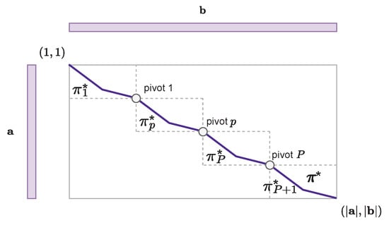
Figure 4.
Computation of the optimal path between pivots with the textbook alignment algorithm.
The problem is thus reduced to a pivot search with linear memory requirements.
3.2.2. Pivot Search
Let denote the number of diagonals with slope of the matrix (more precisely, anti-diagonals, but we use the term diagonal interchangeably in this sense for brevity). Let denote the values of the diagonal of the matrix, as depicted in Figure 5.
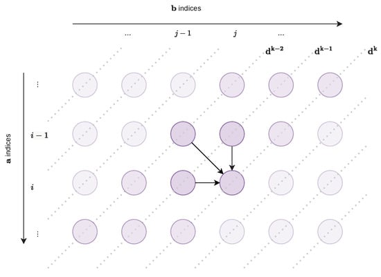
Figure 5.
At least one point of the optimal path also lies on any pair of diagonals and .
Given the permitted transitions, it is straightforward to observe that we need two diagonals to be sure that at least one point of these two diagonals also lies on the optimal path. Therefore, for a given k, there is at least one point on the pair of diagonals and that also lies on the optimal path and that can be used as a pivot.
3.2.3. Pivot Search on and
The point on or with the maximal alignment measure only reflects the local optimal alignment between the corresponding prefixes of sequences and , not between the entire sequences and . This point is thus not necessarily on the optimal path.
Let and denote the sequences and taken in the reversed order, and let denote the alignment measure between the prefixes and . Tralie and Dempsey demonstrated that the optimal alignment measure of Equation (5) can be re-formulated as:
In other terms, for any point on the optimal path, the global optimal alignment measure between and is equal to the alignment measure from to this point , plus the alignment measure in reversed order from to this point , minus the similarity measure at , otherwise counted twice.
For a given k, there is at least one point on the pair of diagonals or that also lies on the optimal path and that can be used as a pivot: it is the point maximised in the right hand side of Equation (8), by definition of the optimal alignment measure:
To compute the right hand side of Equation (8), for all points belonging to and , let denote the diagonal of the matrix. Importantly, note that the diagonal (respecting ) and (respecting ) overlap, as depicted on Figure 6. For a given k, the computation of the diagonals , in a forward direction, and and in a backward direction is therefore enough to find the corresponding pivot.
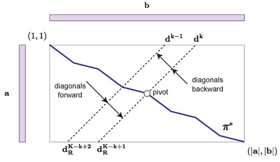
Figure 6.
Pivot search given , , , and .
3.2.4. Diagonal Computation with Linear Memory Complexity
Tralie and Dempsey proposed to compute recursively, noticing that Equation (6) can be computed recursively diagonal-wise, instead of row- and column-wise. The permitted transitions depicted on Figure 3 are demonstrated for the diagonal-wise computation on Figure 5. It is straightforward to observe that can be computed knowing and .
The key idea is that once as been computed, only the values of and are needed to compute the next diagonal , and can be dropped. From an implementation perspective, each diagonal memory buffer pointer is shifted circularly at each step (, , ). Only three diagonal memory buffers are thus necessary to compute all diagonals. As a diagonal has a maximal length of , the linear memory requirement of this recursion scales linearly in .
The same reasoning applies to compute recursively diagonal-wise.
3.3. The CTC Alignment Algorithm
The concept of the Connectionist Temporal Classification (CTC) was first developed by Graves et al. [31] to train a neural network for the task of labelling unsegmented data. In this subsection, we summarize the main ideas developed by Graves et al. that are important for our purpose and we refer the interested reader to the original paper for the detailed description of the CTC algorithm. We then describe how CTC and DTW are related.
3.3.1. Definitions
Let denote a finite alphabet of labels, and denote the set of label sequences, called labellings. We also define , where is a blank label, and let denote the set of sequences of labels and blanks, subsequently called the labelling extension or simply extensions.
Let denote the many-to-one function mapping different extensions of length T to a single labelling of length by removing the successive duplicated labels and blanks. For instance, the following different extensions are mapped to the same labelling:
A connectionist temporal classifier (CTC) is a neural network whose input is a feature sequence , and whose output is a tensor, called a posteriorgram. The last layer is a softmax layer applied on the first dimension; thus, each timeframe at instant t is interpreted as the probability mass function of the label discrete probability distribution over . More precisely, if we denote , the output corresponding to the label at time t, represents the probability of observing label k at time t, given the input sequence .
A posteriorgram thus defines a distribution over the set of possible labelling extensions of length T, as visualized on Figure 7. The conditional probability of a given labelling extension is thus:
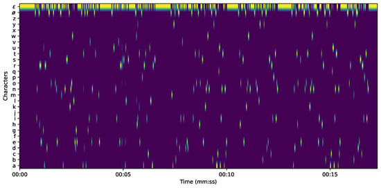
Figure 7.
The posteriorgram of the first sentence of chapter 10 of “The problems of philosophy”, by B. Russell. Audio publicly available on Librivox. See Section 4.2 for details.
The conditional probability of any labelling of is thus the sum of the probability of all its corresponding extensions:
A CTC network is trained to find the most likely labelling , maximising Equation (13):
The objective function of Equation (13), called the CTC loss, is usually intractable in its direct form, because a labelling has typically too many extensions. The idea proposed by Graves et al. was to compute the probability in Equation (13) recursively, similarly to what was conducted with the alignment measure of Equation (5).
Consider the first labels in . By definition of the extensions, there are different possibilities for the next label, depending on whether the last one is blank or non-blank:
- If it is a blank label , the next label can be or the next non-blank label .
- If it is a non-blank label , the next label can either be the same label , the blank label , or the next label, , if .
These permitted transitions are depicted in the Figure 8.
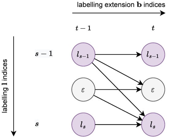
Figure 8.
CTC labelling-permitted extensions.
The trick proposed by Graves et al. to account for transitions to and from in Figure 8 was to consider a new sequence obtained interleaving between each label pair of , and adding at the beginning and the end. Consequently, , and if we let i denote the index of , , as depicted in Figure 9.
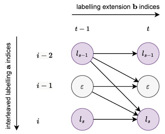
Figure 9.
CTC path-permitted transitions.
3.3.2. Computation via Dynamic Programming
The reasoning is similar to that followed to obtain the recurrence equation, Equation (6). As shown on Figure 9, if the optimal path between two sequences passes through the point , it necessarily passes through one of the points , , or . It is thus enough to know the probability of these 3 predecessor to deduce the probability on the point .
Let denote the total probability to have the prefix corresponding to the prefix , and assume that , , and are already known. Given the permitted path transitions depicted on Figure 9, it is straightforward to observe that:
The initialisation step is given by:
Finally, an extension can terminate with or the last label ; thus, the probability is the sum of the total probability of with or without the last :
In their seminal paper, Graves et al. introduced to compute , i.e., the CTC loss of Equation (13), with the objective to differentiate it with respect to the network weight for back-propagation training. For our present purpose, it is enough to compute . We refer the interested reader to the original paper for details about CTC loss differentiation.
3.3.3. CTC-Forced Alignment
The matrix in Equation (15) is computed over all possible paths , because it is used to compute the CTC loss (see Equation (17) and Equation (13)). In the CTC-forced alignment scenario, the labelling is given, and we search for an optimal , maximising the probability , as in the textbook DTW scenario.
The Equation (15) is thus slightly modified, so that only the predecessor path with the maximal probability is considered at each step, and becomes:
The probability can then be computed recursively using Equations (16) and (18), accumulating at each step the probability of the most probable predecessor path (forward pass). The optimal path can then be traced back using the sequence of optimal transitions retained in the forward pass (backward pass).
Similarly to the textbook DTW algorithm, the computation of the matrix in a CTC context given by Equation (18) during the forward pass has a computational and memory complexity that scales quadratically in , i.e., .
3.4. Linear Memory CTC Alignment
In this subsection, we present our adaptation of the linear memory DTW algorithm to the CTC context. The divide-and-conquer strategy remains the same: search for pivots and compute the optimal path between pivots with the quadratic CTC-decoding algorithm. Only the aspects related to the permitted transitions have to be adapted.
3.4.1. Pivot Search
The pivot search in a CTC context is directly adapted from the textbook DTW context, taking into account the CTC permitted transitions depicted on Figure 8, and shown for the diagonal-wise computation in Figure 10.
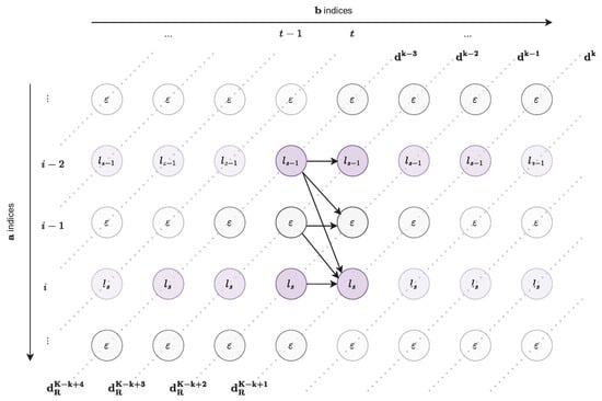
Figure 10.
At least one point of the optimal path also lies on any triplet of diagonals , , .
Given the permitted transitions, it is straightforward to observe that we need three diagonals to be sure that at least one point of these three diagonals also lies on the optimal path. Therefore, for a given k, there is at least one point on the triplet of diagonals , , and that also lies on the optimal path and that can be used as a pivot.
3.4.2. Pivot Search on , , and
The same reasoning described for the DTW context applies to the CTC context. In particular, the Equation (8) remains valid in a CTC context, replacing the similarity measure with log-probability:
For a given k, there is at least one point on the triplet of diagonals , , or that also lies on the optimal path and that can be used as pivot: it is the point maximising Equation (19) on the right hand side, by definition of the optimal alignment measure:
For a given k, the computation of the diagonals , , and in a forward direction, and of , , and in a backward direction, is therefore enough to find the corresponding pivot.
3.4.3. α and αR Computation Diagonal-Wise
Similarly to the textbook DTW case, the Equation (15) can be computed recursively diagonal-wise, instead of row- and column-wise, and it is straightforward to observe from Figure 10 that the values of can be directly computed given the values of , , and .
The recurrence rule in Equation (15) can be rewritten as:
and the initialisation step Equation (16) becomes:
Similarly to the textbook DTW case, once has been computed, only the values of , , and are needed to compute the next diagonal , and can be dropped. Using the memory buffer circular shift already described, the requirement of this recursion scales linearly in . In the case of an audio to text alignment, there are generally much less labels than posteriorgram frames, i.e., ). The memory requirement of the algorithm therefore scales linearly in , i.e., .
The same reasoning applies to compute recursively diagonal-wise.
3.5. Neural Architecture
In this subsection, we describe the neural network trained with a CTC loss implementing the encoding step , depicted in Figure 1.
3.5.1. Inputs
The network takes as inputs normalized log-mel-spectrograms that are derived from the audio. First, all audio data are resampled to 16 kHz and processed by computing a 1024-bin Fast Fourier Transform on successive 1024-long Hanning windows shifted every 512 samples. Therefore, each of the T spectrogram frames has a duration of 32ms. The linear frequency scale is compressed into Mel bins.
3.5.2. Architecture
Our model is depicted on Figure 11. It contains a succession of 8 convolutional blocks. Each block contains 2 sub-blocks, composed of the following layers: batch normalization, 2D-convolution with kernels and same padding, batch normalization, ReLU activation, and 20% dropout. No pooling is used. In each block, the first sub-block convolution uses stride, but the second one uses a stride, hence halving the number of bins on the frequency axis. Each block increases the number of filters . In total, the model has thus 16 convolutional layers, but changes the number of frequency bins and channels every two layers only.
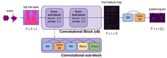
Figure 11.
Fully convolutional neural network generating posteriorgram from log-mel spectrograms.
Note that the global receptive field of the 16 convolutional layers is about 1 s. Therefore, the model can be trained on audio excerpts with durations of several seconds (typically between 10–20 s), but can be used in inference on several hours of audio thanks to its fully convolutional architecture.
3.5.3. Output
The resulting feature map, which is an element of with , is finally turned into the posteriorgram thanks to a final batch normalization and 2D-convolution. A softmax activation is applied to obtain the per-frame probability distributions over the labels.
In this work, we considered an alignment at the word level, i.e., subsequences of characters separated by the space symbol ∅. We therefore defined the alphabet of labels to include the characters [a–z] and the space symbol ∅. The start index of each word in the posteriorgram is thus given by the index t of the first non-space label directly following a space label. The actual timestamp of each word can then easily be deduced knowing the duration of each posteriorgram frame.
4. Experiments and Results
In this section, we present our experiments both for spoken and singing voice alignment. We first provide the model training details, then present the corpora that we built to evaluate our system performances, and the standard metrics that we report [64]. We then present our results on very long audio alignment tasks, and investigate the robustness of the system against corrupted reference text corruption and multiple languages. We finally compare our results to current state-of-the-art algorithms.
4.1. Model Training
We conducted two series of experiments, one for speech and the other for singing voice. We used the same model architecture, defined as Section 3.5, for both series.
4.1.1. Speech
We used the train-clean-100, train-clean-360, and train-other-500 sets of Librispeech (https://www.openslr.org/12 (accessed on 31 January 2023)) for training, and the dev-clean set for evaluation. The model was trained during 50 epochs via a classical CTC loss, Adam optimizer, initial learning rate of with 5 epochs of warm up, and an exponential decay with a factor of 0.9 each time the loss did not decrease on the evaluation set for 2 epochs after the warm up. We used a batch size of 32 × 4 on 4 GPUs Tesla V100-SXM2-32GB. The training lasted roughly 16 h.
4.1.2. Singing voice
We used a 90-10 split of the DALI dataset (https://github.com/gabolsgabs/DALI (accessed on 31 January 2023)) for training and evaluation. The model was trained during 200 epochs (with 512 steps per epoch) via the classical CTC loss, Adam optimizer, and initial learning rate of that is reduced by a factor of 0.9 each time the loss did not decrease on the evaluation set for 2 epochs. We used a batch size of 16 on 1 GPUs NVIDIA GeForce GTW 1080 Ti with 12 MB. The training lasted roughly 10 h.
4.2. Reference Corpora
There is no publicly available corpora to assess the performances of systems addressing the very long audio alignment task. Therefore, we assembled such corpora for the spoken and singing voice, and released them publicly (https://ircam-anasynth.github.io/papers/2023/a-linear-memory-ctc-based-algorithm-for-text-to-voice-alignment-of-very-long-audio-recordings (accessed on 31 January 2023)). We encourage the community to use them.
4.2.1. Speech
For speech, we manually annotated the audio recording of a whole chapter of a publicly available audiobook. We choose the chapter 10 of The Problems of Philosophy, by B. Russell (https://librivox.org/the-problems-of-philosophy-by-bertrand-russell-2/ (accessed on 31 January 2023)). This audiobook does not belong to the Librispeech’s list of books, and its reader does not belong to the Librispeech’s list of readers either (https://www.openslr.org/resources/12/raw-metadata.tar.gz (accessed on 31 January 2023)). The chapter 10 contains exactly 100 sentences and 2672 words, and the corresponding audio has a duration of 21:05 (MM:SS). The other chapters were kept for our experiments (see below).
We first removed from the audio the Librivox preamble with the title and copyright information. Then, we performed a first alignment of the audio with the available text with our algorithm, which we used as a starting point to manually and precisely align each word to the audio. During the alignment process, we corrected a few inconsistencies between the recording and the transcription, so that text and audio match exactly. The alignment was conducted by adjusting the markers for the start of each word. We used the spectrogram representation to precisely align the start of the words with the corresponding onsets. In the following, we will refer to this spoken voice reference corpus as “Chapter 10”.
4.2.2. Singing Voice
For singing, we leveraged the available annotations of the DALI dataset, in which all of the alignments have already been annotated at the word level [45]. We selected 150 songs that were not used during our model training, and we gathered a playlist containing 50 of these songs. We simply concatenated both the audio and the corresponding annotated lyrics available in DALI. The playlist contains 18,094 words, and the corresponding audio has a duration of 2:50:24 (HH:MM:SS). The other 100 songs were kept for our experiments (see below).
In the following, we will refer to this singing voice reference corpus as “Playlist 50”.
4.3. Evaluation Metrics
In order to evaluate the performances of our models, we compute several metrics presented below. Note that we only consider the word onsets as decision boundaries, i.e., we do not compute errors neither on space (character ∅) onsets/offsets nor word offsets.
The Mean Absolute Alignment Error (MAAE) is the most used metric in alignment evaluations. It reports the average value of all Absolute Alignment Errors (AAE), that measure the absolute difference between the predicted and true times of each word onset.
The Quantile N (QN%) metric reports, for a fixed , the Nth quantile of Absolute Alignment Error (AAE) over all word onsets, indicating that N% of the AAE are below the value QN%. In opposition to the MAAE, this metric is insensitive to outliers. In our evaluations, we will compute the N = 50 (median AAE), N = 95, and N = 99 quantiles.
The Percentage of Correct Onsets (PCO) metric measures the percentage of onsets that can be considered correctly aligned. A threshold of 300 ms is commonly admitted and chosen by the community for the misaligned/well-aligned binary decision [44,64], which we choose as well.
4.4. Baseline Results
We first evaluated the performances of our speech and singing voice alignment models. The Absolute Alignment Error (AAE) obtained on each words of the reference corpus has been computed, and the distribution is shown in Figure 12.
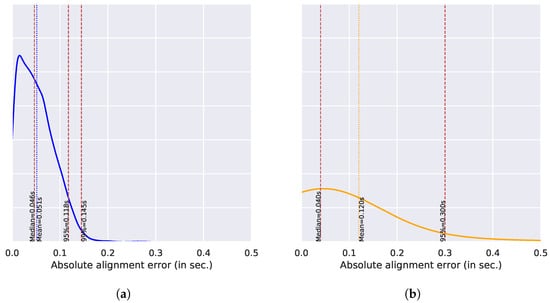
Figure 12.
Absolute alignment error distribution. (a) Speech (Chapter 10); (b) Singing (Playlist 50).
In Figure 12a, the AAE distribution for speech is shown. The mean of AAE (MAAE) is of 46ms, close to the median (51ms). Even the most severe outliers (quantiles 95% and 99%) remain below 150 ms. The Percentage of Correct Onsets (PCO) is 100%, as there is not a single AAE value greater than 300 ms.
The AAE distribution for the singing voice is shown in Figure 12b. The mean of the AAE (MAAE) is 120 ms and is therefore three times higher than for speech. This is clearly due to the more challenging context (i.e., singing word recognition, longer pauses, and musical accompaniment) that leads to extreme outliers, with some AAE even greater than 1.2 s, which naturally impact the mean value. However, the median (around 40 ms) remains in the same order of magnitude as the one reported for speech. The Percentage of Correct Onsets (PCO) is 95%.
The MAAE obtained for the speech and singing voice will serve as a comparison baseline in the following experiments.
4.5. Effect of Audio Duration and Number of Words on Performances
In this section, we investigate the effect of the longer audio–text pair on the baseline alignment accuracy. This is where we explicitly tackle the task of very long audio-to-text alignment at the word level.
For speech, we added the three chapters before and/or after the reference Chapter 10 to produce longer data. We thus performed the alignment between the audio and the corresponding text for Chapters 7–10, Chapters 10–13, and Chapters 7–13. For the singing voice, we added 50 songs before and/or after the Playlist 50. We thus performed the alignment between the audio and the corresponding lyrics for up to 150 songs.
We computed the alignment on a single Intel(R) Xeon(R) Gold 5118 CPU @ 2.30GHz on a server with 131.6 GB RAM. We rely on the linear memory-forced alignment that we presented in Section 3.4 to deal with long audio-text context. We systematically report the number of pivots that we use.
We computed the AAE for Chapter 10 and Playlist 50 for each case, taking the offsets incurred by the other chapters/songs. The results are shown in Table 1 and Table 2.

Table 1.
Absolute alignment error on Chapter 10 for alignments of several chapters.
Table 2.
Absolute alignment error on Playlist 50 (P50) for alignments with 50 to 100 extra songs.
These results demonstrate that the alignment error remains remarkably stable, both for speech and the singing voice, even when preceded and/or followed by several extra hours of audio and the corresponding transcripts. This indicates that the system is able to precisely align several hours of audio with the corresponding text and with the same level of accuracy.
The encoding module is insensitive to increasing audio duration thanks to its fully convolutional architecture. The forced-alignment module is also insensitive to increasing audio duration and corresponding transcript length thanks to the use of pivots.
4.6. Effect of Text Transcription Errors on Performances
In practice, audio transcriptions typically contain errors. For instance, words can contain typos, i.e., one or several characters might have been added, removed, or altered, or entire words could be added or removed. In this section, we investigate the effect of transcription errors on the alignment accuracy obtained for Chapter 10 and Playlist 50.
4.6.1. Effect of Replaced Characters
We replace p% of the characters uniformly at random in the text of Chapter 10 and Playlist 50, leaving the space characters untouched so the number of words remains the same. The new characters are sampled uniformly at random in the [a–z] letters. We perform the alignment of the altered text again with the original audio posteriorgram (which is not impacted by transcript alterations).
The alignment error for speech is shown on Figure 13a. It remains remarkably stable around the baseline up to 50% of replaced characters. The error even remains under the 200 ms error for up to 80% of substitutions, but dramatically rises after that. The system is thus able to compensate for transcription errors, as long as it obtains enough correct anchorage characters.
Figure 13.
Mean absolute alignment Error for different percentages of replaced characters. (a) Speech (Chapter 10); (b) Singing (Playlist 50).
The alignment error for the singing voice is shown on Figure 13b. It increases much faster than for speech, even for a small percentage of replaced characters: due to the presence of musical accompaniment, the posteriorgram exhibits less clear-cut character probabilities, which causes the correct anchor characters to be more easily confused with wrong characters and the optimal alignment path to diverge faster.
4.6.2. Effect of Added/Removed Characters
We remove or add p% of the characters uniformly at random in the text of Chapter 10 and Playlist 50, leaving the space characters untouched, so the number of words remains the same. When p decreases towards −100%, it becomes likely that several characters will be removed on each word; thus, we make sure that each word retains at least one character. We perform the alignment of the altered text again with the audio posteriorgram.
Figure 14a shows that the alignment error on speech remains remarkably stable around the baseline, and for up to 50% of the added/removed characters. The error increases steadily when adding extra characters, as expected. More surprisingly, the error decreases slightly, as compared to the baseline when removing 0–50% of the characters. One interpretation is that removing some characters could be beneficial for the CTC decoding if the model fails to recognize them properly. When more than 50% of the characters are removed, the error increases again. Interestingly, the MAAE always remains under 200 ms, even after each word contains only one single character. This indicates that the space character is a very powerful anchor, and plays a crucial role in aligning the text with the posteriorgram.
Figure 14.
Mean absolute alignment error for different percentages of removed/added characters. (a) Speech (Chapter 10); (b) Singing (Playlist 50).
Figure 14b shows that the singing aligner is much more sensitive to these kind of character alterations. Similarly to the character replacement in the previous experiment, we observe that the singing voice is much more sensitive than speech to the altered transcriptions. As in the previous, this can be explained by the fact that anchor characters are more ambiguous than for plain speech, which causes the optimal path to diverge more easily.
4.6.3. Effect of Added/Removed Words
Finally, we remove or add p% of the words uniformly at random in the text of Chapter 10 and Playlist 50. For each added word, we first sample a length l following a normal distribution centered around a mean length of six characters, and then generate a word of l sampled uniformly at random in the [a–z] letters. As removed or added words are not present in our manually aligned reference, we compute the AE only for the original words of Chapter 10 and Playlist 50, respectively.
Figure 15a shows the speech MAAE for different values of p. It shows that the alignment error remains under the 200 ms error even if half of the words are missing or added. This indicates that the alignment is very robust to noise, as long as more than half of the true words remain untouched. Beyond that point, there are not enough words to keep the alignment stable, and the error increases dramatically.
Figure 15.
Mean absolute alignment error for different percentages of removed/added words. (a) Speech (Chapter 10); (b) Singing (Playlist 50).
Similarly to the previous experiments, Figure 15b shows that the singing voice alignment is much more sensitive to a full word addition or deletion. As in the previous, this can be interpreted by the fact that the posteriorgram does not exhibit sufficiently salient probabilities for correct characters in order to provide steady anchorage compensating for transcription errors.
4.7. Different Languages
Our models were trained for English only (both on Librispeech and DALI). In this section, we investigate the performances of these models applied to other languages.
4.7.1. Speech
We selected from the Librivox corpus several audiobooks in other languages than English, listed in Table 3. For each language, the text corresponding to approximately 1 min of audio was manually aligned by native speakers. We publicly released the audio and the manually aligned transcript for each language (https://ircam-anasynth.github.io/papers/2023/a-linear-memory-ctc-based-algorithm-for-text-to-voice-alignment-of-very-long-audio-recordings (accessed on 31 January 2023)).
Table 3.
Comparing the alignment performances of our CTC-based aligner (trained in English) on speech in different languages. * The text in these languages has been transliterated to Latin alphabet before alignment.
For Latin alphabet languages, diacritic characters are converted to plain characters with the python unidecode package (https://pypi.org/project/Unidecode (accessed on 31 January 2023)). For non-Latin alphabet languages, the text was first transliterated before the synchronisation: for Chinese, we used the python pinyin package (https://pypi.org/project/pinyin (accessed on 31 January 2023)), for Greek, we used the python polyglot package (https://github.com/aboSamoor/polyglot (accessed on 31 January 2023)), and for Arabic, we used a human manual transliteration. We used our system to align the text to the audio, and summarized the results in Table 3.
It appears that although the system was trained in English audio and transcripts only, it performs very well for other languages as well, including for languages that have a very distinct pronunciation, as compared to English. We interpret these results by the fact that the system encounters enough anchor characters (typically spaces, vowels, and consonants that are common to English) to align the full words correctly, even though it might not be able to recognize some particular phonemes perfectly. The variations in the MAAE between languages is in fact mainly related to the clear or unclear articulation of the words, as can be heard on the videos available on our companion website.
4.7.2. Singing Voice
We evaluate the singing alignment on the five most prominent languages in DALI, which are English, French, German, Italian, and Spanish. We used a five-fold evaluation strategy on 50 songs (the same as for our baseline Playlist 50). However, we measure the alignment error on each song, not their concatenation as for Playlist 50, and report the average metrics on Table 4. The DALI track IDs for these additional languages are also available on our companion website.
Table 4.
Comparing the alignment performances of our CTC-based aligner (trained in English) on singing voice in different languages.
For English, we obtain similar results to that obtained for Playlist 50. As each song here is evaluated individually and as it is simpler to perform a short than long alignment, we even obtain slightly better performances. However, performances clearly degrade in other languages. In fact, there exist extremely severe outliers (Q95% and Q99% metrics) that naturally degrade the MAAE. When analyzing some of them, we observe cases in which the first word of the next paragraph is predicted at the beginning of a long instrumental bridge, or a word is emitted because of background vocals that are not part of the original transcript.
An interesting conclusion, though, is that the median error remains under 100 ms for all languages. Since it will always be hard to account for the huge diversity existing for the singing voice in song recordings, the median value is certainly a better metric than MAAE to assess alignment performances in the singing voice, especially with background music.
4.8. Performance Benchmark
Alignment performance evaluations available in the literature are usually conducted on relatively short audio durations, and, to the best of our knowledge, there is no common evaluation set for long audio alignment. However, we provide in this subsection some performance benchmarks.
4.8.1. Comparison with Other ASR Systems
We re-implemented the well-known ASR system Wav2Letter [33,65], and compared its performance with our baseline model. We evaluated the speech recognition performances on the dev-clean set of the Librispeech by means of the Character Error Rate (CER) and Word Error Rate (WER), and the alignment performances in Chapter 10, as described in Section 4.4, and as reported in Table 5.
Table 5.
Performance comparison of our model vs. Wav2Letter.
The results for speech recognition are much better for Wav2Letter, which was expected, as it was specially designed for this task and has three times more parameters than our model. Surprisingly, however, the Wav2Letter alignment performances are not as good as those of our model. This indicates that plain- and forced- CTC decoding provides different optimal paths for each task at hand.
4.8.2. Comparison with Other Alignment Systems
The classical datasets used in the MIREX contest (https://www.music-ir.org/mirex/wiki/2020:Automatic_Lyrics-to-Audio_Alignment_Results (accessed on 31 January 2023)), i.e., Jamendo and Hansen’s datasets, only include up to 20 songs of a few minutes. Although our system was designed to address the very long audio alignment use case, we compared our system with the current state-of-the-art systems for the sake of completeness, as reported in Table 6. For this experiment, our model was trained on the entire DALI dataset, with each epoch processing the whole database. The rest of the above-mentioned training procedure remains identical.
Table 6.
Lyrics’ alignment MAAE (ms) on the Hansen (a cappella variant) and Jamendo datasets and comparison to the latest alignment systems (MIREX 2020). We indicate best performing version on each dataset, as reported on MIREX 2020 results (https://www.music-ir.org/mirex/wiki/2020:Automatic_Lyrics-to-Audio_Alignment_Results (accessed on 31 January 2023)).
Comparing first the results of the Jamendo dataset, we find that our system is second in MAAE, with a Q50% value equal to the best SOTA result. For the a cappella variant of the Hansen dataset, our system achieves results close to the second-best SOTA system. Note that all SOTA systems involve acoustic and language models, while our system relies on a simpler end-to-end architecture.
5. Conclusions
Popular applications such as automatic closed-captioning or karaoke generally come to mind when mentioning text-to-voice synchronization. However, it also plays an increasingly important role in the academic field by generating an automatically large corpora of paired voice and text for downstream tasks, such as voice synthesis or speaker identity change.
Text-to-voice synchronization algorithms typically consist of two steps: an encoding step, where a time series of symbols is inferred from the audio, and a forced-alignment step, where these symbol timestamps are assigned to the ground-truth text. We presented in this work a novel algorithm, where the encoding module is implemented as a fully CTC-based convolutional network, and where the forced-alignment module is implemented as a CTC decoder with linear memory complexity.
We demonstrated that this approach is able to align the text to several hours of audio with a mean alignment error of 50 ms for speech, and 120 ms for the singing voice. We also demonstrated that the system is robust for increasing audio durations, as well as severe ground-truth text alterations, such as character and word insertions or deletions. We interpreted these performances by the fact that the system only requires a minimal amount of correct characters that serve as anchors to align the entire text correctly. This also explains that the system, albeit trained solely in English text, obtains a similar accuracy with other languages for speech and, to a lesser extent, with the singing voice.
In the future, we plan to speed up the algorithm by adapting the forced-alignment step for GPU parallelization. We also plan to generate and publicly release a large corpora of synchronized text and voice for future research.
Author Contributions
Conceptualization, G.D., Y.T. and A.R.; methodology, G.D.; software, G.D. and Y.T.; validation, G.D., Y.T. and A.R.; formal analysis, G.D.; investigation, G.D.; resources, A.R.; data curation, G.D. and Y.T.; writing—original draft preparation, G.D. and Y.T.; writing—review and editing, G.D., Y.T. and A.R.; visualization, G.D. and Y.T.; supervision, A.R.; project administration, A.R.; funding acquisition, A.R. All authors have read and agreed to the published version of the manuscript.
Funding
This research was partly funded by the French National Research Agency (Agence Nationale de la Recherche—ANR) as part of the ARS project (ANR-19-CE38-0001-01).
Institutional Review Board Statement
Not applicable.
Informed Consent Statement
Not applicable.
Data Availability Statement
The Librispeech dataset can be found at https://www.openslr.org/12 (accessed on 31 January 2023). The DALI dataset can be found at (https://github.com/gabolsgabs/DALI (accessed on 31 January 2023). The evaluation dataset (Chapter 10 and Playlist 50) are available at https://ircam-anasynth.github.io/papers/2023/a-linear-memory-ctc-based-algorithm-for-text-to-voice-alignment-of-very-long-audio-recordings (accessed on 31 January 2023).
Acknowledgments
The authors are very thankful to (1) Christopher Tralie for fruitful discussions about the linear memory DTW; and (2) Jan Chab, Christina Chalastanis, Alice Cohen-Hadria, Paola Lumbroso, Klarissa Roebel, Mei-Hua Roebel, Léane Salais, Georgia Spiropoulos, and Marc Wijnand, for manually aligning text-to-voice in their respective mother tongue.
Conflicts of Interest
The authors declare no conflict of interest. The funders had no role in the design of the study; in the collection, analyses, or interpretation of data; in the writing of the manuscript; or in the decision to publish the results.
References
- Viterbi, A. Error bounds for convolutional codes and an asymptotically optimum decoding algorithm. IEEE Trans. Inf. Theory 1967, 13, 260–269. [Google Scholar] [CrossRef]
- Needleman, S.B.; Wunsch, C.D. A general method applicable to the search for similarities in the amino acid sequence of two proteins. J. Mol. Biol. 1970, 48, 443–453. [Google Scholar] [CrossRef] [PubMed]
- Vintsyuk, T.K. Speech discrimination by dynamic programming. Cybernetics 1968, 4, 52–57. [Google Scholar] [CrossRef]
- Velichko, V.; Zagoruyko, N. Automatic recognition of 200 words. Int. J. Man-Mach. Stud. 1970, 2, 223–234. [Google Scholar] [CrossRef]
- Itakura, F. Minimum prediction residual principle applied to speech recognition. IEEE Trans. Acoust. Speech Signal Process. 1975, 23, 67–72. [Google Scholar] [CrossRef]
- Mongeau, M.; Sankoff, D. Comparison of musical sequences. Comput. Humanit. 1990, 24, 161–175. [Google Scholar] [CrossRef]
- Orio, N.; Schwarz, D. Alignment of monophonic and polyphonic music to a score. In Proceedings of the International Computer Music Conference (ICMC), Havana, Cuba, 17–22 September 2001. [Google Scholar]
- Müller, M.; Kurth, F.; Clausen, M. Audio Matching via Chroma-Based Statistical Features. In Proceedings of the ISMIR (International Society for Music Information Retrieval), London, UK, 11–15 September 2005. [Google Scholar]
- Ellis, D.P. Beat Tracking with Dynamic Programming. J. New Music. Res. 2007, 36, 51–60. [Google Scholar] [CrossRef]
- Serrà, J.; Gómez, E. A cover song identification system based on sequences of tonal descriptors. MIREX (Music Information Retrieval Evaluation eXchange); Citeseer: Princeton, NJ, USA, 2007; Volume 46. [Google Scholar]
- Wagner, M. Automatic labelling of continuous speech with a given phonetic transcription using dynamic programming algorithms. In Proceedings of the IEEE International Conference on Acoustics, Speech, and Signal Processing (ICASSP’81), Atlanta, GA, USA, 30 March–1 April 1981; Volume 6, pp. 1156–1159. [Google Scholar]
- Leung, H.; Zue, V. A procedure for automatic alignment of phonetic transcriptions with continuous speech. In Proceedings of the IEEE International Conference on Acoustics, Speech, and Signal Processing (ICASSP’84), San Diego, California, USA, 19–21 March 1984; Volume 9, pp. 73–76. [Google Scholar]
- Ljolje, A.; Riley, M. Automatic segmentation and labeling of speech. In Proceedings of the IEEE International Conference on Acoustics, Speech, and Signal Processing, Toronto, ON, Canada, 14–17 April 1991; pp. 473–476. [Google Scholar]
- Placeway, P.; Lafferty, J. Cheating with imperfect transcripts. In Proceeding of Fourth International Conference on Spoken Language Processing (ICSLP’96), Philadelphia, PA, USA, 3–6 October 1996; Volume 4, pp. 2115–2118. [Google Scholar]
- Moreno, P.J.; Joerg, C.; Thong, J.M.V.; Glickman, O. A recursive algorithm for the forced alignment of very long audio segments. In Proceedings of the Fifth International Conference on Spoken Language Processing, Sydney, Australia, 30 November–4 December 1998. [Google Scholar]
- Hazen, T.J. Automatic alignment and error correction of human generated transcripts for long speech recordings. In Proceedings of the Ninth International Conference on Spoken Language Processing, Pittsburgh, PA, USA, 17– 21 September 2006. [Google Scholar]
- Katsamanis, A.; Black, M.; Georgiou, P.G.; Goldstein, L.; Narayanan, S. SailAlign: Robust long speech-text alignment. In Proceedings of the Workshop on New Tools and Methods for Very-Large Scale Phonetics Research, Philadelphia, PA, USA, 29–31 January 2011. [Google Scholar]
- Anguera, X.; Perez, N.; Urruela, A.; Oliver, N. Automatic synchronization of electronic and audio books via TTS alignment and silence filtering. In Proceedings of the 2011 IEEE International Conference on Multimedia and Expo, Barcelona, Spain, 11–15 July 2011; pp. 1–6. [Google Scholar]
- Hoffmann, S.; Pfister, B.; Text-to-speech alignment of long recordings using universal phone models. INTERSPEECH. Citeseer. 2013, pp. 1520–1524. Available online: https://citeseerx.ist.psu.edu/document?repid=rep1&type=pdf&doi=c2de617d6eeb82cba0fe7e1453d4ab9a354d3d78 (accessed on 31 January 2023).
- Ruiz, P.; Álvarez, A.; Arzelus, H. Phoneme similarity matrices to improve long audio alignment for automatic subtitling. In Proceedings of the Ninth International Conference on Language Resources and Evaluation (LREC), Reykjavik, Iceland, 26–31 May 2014. [Google Scholar]
- Álvarez, A.; Arzelus, H.; Ruiz, P. Long audio alignment for automatic subtitling using different phone-relatedness measures. In Proceedings of the 2014 IEEE International Conference on Acoustics, Speech and Signal Processing (ICASSP), Florence, Italy, 4–9 May 2014; pp. 6280–6284. [Google Scholar]
- Bordel, G.; Penagarikano, M.; Rodríguez-Fuentes, L.J.; Álvarez, A.; Varona, A. Probabilistic kernels for improved text-to-speech alignment in long audio tracks. IEEE Signal Process. Lett. 2015, 23, 126–129. [Google Scholar] [CrossRef]
- Gupta, C.; Yılmaz, E.; Li, H. Automatic Lyrics Alignment and Transcription in Polyphonic Music: Does Background Music Help? In Proceedings of the ICASSP 2020—2020 IEEE International Conference on Acoustics, Speech and Signal Processing (ICASSP), Barcelona, Spain, 4–8 May 2020; pp. 496–500. [Google Scholar]
- Mohamed, A.r.; Dahl, G.E.; Hinton, G. Acoustic modeling using deep belief networks. IEEE Trans. Audio Speech Lang. Process. 2012, 20, 14–22. [Google Scholar] [CrossRef]
- Graves, A.; Mohamed, A.r.; Hinton, G. Speech recognition with deep recurrent neural networks. In Proceedings of the 2013 IEEE International Conference on Acoustics, Speech and Signal Processing (ICASSP), Vancouver, BC, Canada, 26–31 May 2013; pp. 6645–6649. [Google Scholar]
- Hannun, A.; Case, C.; Casper, J.; Catanzaro, B.; Diamos, G.; Elsen, E.; Prenger, R.; Satheesh, S.; Sengupta, S.; Coates, A.; et al. Deep speech: Scaling up end-to-end speech recognition. arXiv 2014, arXiv:1412.5567. [Google Scholar]
- Kelley, M.C.; Tucker, B.V.; A comparison of input types to a deep neural network-based forced aligner. Interspeech 2018. Available online: https://era.library.ualberta.ca/items/0fbd7532-1105-4641-9e12-ebb0e349e460/download/169d5d27-d3a6-411e-ad6d-320032130103 (accessed on 31 January 2023).
- Backstrom, D.; Kelley, M.C.; Tucker, V.B. Forced-alignment of the sung acoustic signal using deep neural nets. Can. Acoust. 2019, 47, 98–99. [Google Scholar]
- Schulze-Forster, K. Informed Audio Source Separation with Deep Learning in Limited Data Settings. Ph.D. Thesis, Institut Polytechnique de Paris, Palaiseau, France, 2021. [Google Scholar]
- Schulze-Forster, K.; Doire, C.S.; Richard, G.; Badeau, R. Phoneme level lyrics alignment and text-informed singing voice separation. IEEE/ACM Trans. Audio, Speech, Lang. Process. 2021, 29, 2382–2395. [Google Scholar] [CrossRef]
- Graves, A.; Fernández, S.; Gomez, F.; Schmidhuber, J. Connectionist temporal classification: Labelling unsegmented sequence data with recurrent neural networks. In Proceedings of the 23rd International Conference on Machine Learning, Pittsburgh, PA, USA, 25–29 June 2006; pp. 369–376. [Google Scholar]
- Graves, A.; Jaitly, N. Towards end-to-end speech recognition with recurrent neural networks. In Proceedings of the International Conference on Machine Learning, Beijing, China, 21–26 June 2014; pp. 1764–1772. [Google Scholar]
- Collobert, R.; Puhrsch, C.; Synnaeve, G. Wav2letter: An end-to-end convnet-based speech recognition system. arXiv 2016, arXiv:1609.03193. [Google Scholar]
- Zhang, Y.; Pezeshki, M.; Brakel, P.; Zhang, S.; Bengio, C.L.Y.; Courville, A. Towards end-to-end speech recognition with deep convolutional neural networks. arXiv 2017, arXiv:1701.02720. [Google Scholar]
- Hori, T.; Watanabe, S.; Zhang, Y.; Chan, W. Advances in joint CTC-attention based end-to-end speech recognition with a deep CNN encoder and RNN-LM. arXiv 2017, arXiv:1706.02737. [Google Scholar]
- Watanabe, S.; Hori, T.; Kim, S.; Hershey, J.R.; Hayashi, T. Hybrid CTC/attention architecture for end-to-end speech recognition. IEEE J. Sel. Top. Signal Process. 2017, 11, 1240–1253. [Google Scholar] [CrossRef]
- Kim, S.; Hori, T.; Watanabe, S. Joint CTC-attention based end-to-end speech recognition using multi-task learning. In Proceedings of the 2017 IEEE International Conference on Acoustics, Speech and Signal Processing (ICASSP), New Orleans, Lousiana, USA, 5–9 March 2017; pp. 4835–4839. [Google Scholar]
- Stoller, D.; Durand, S.; Ewert, S. End-to-end Lyrics Alignment for Polyphonic Music Using an Audio-to-Character Recognition Model. arXiv 2019, arXiv:1902.06797. [Google Scholar]
- Kürzinger, L.; Winkelbauer, D.; Li, L.; Watzel, T.; Rigoll, G. CTC-segmentation of large corpora for german end-to-end speech recognition. In Proceedings of the International Conference on Speech and Computer, Online, 7–9 October 2020; Springer: Berlin/Heidelberg, Germany, 2020; pp. 267–278. [Google Scholar]
- Tralie, C.; Dempsey, E. Exact, parallelizable dynamic time warping alignment with linear memory. arXiv 2020, arXiv:2008.02734. [Google Scholar]
- Stoller, D.; Ewert, S.; Dixon, S. Wave-u-net: A multi-scale neural network for end-to-end audio source separation. arXiv 2018, arXiv:1806.03185. [Google Scholar]
- Vaglio, A.; Hennequin, R.; Moussallam, M.; Richard, G.; d’Alché Buc, F. Audio-Based Detection of Explicit Content in Music. In Proceedings of the ICASSP 2020—2020 IEEE International Conference on Acoustics, Speech and Signal Processing (ICASSP), Barcelona, Spain, 4–8 May 2020; pp. 526–530. [Google Scholar]
- Vaglio, A.; Hennequin, R.; Moussallam, M.; Richard, G. The words remain the same—Cover detection with lyrics transcription. In Proceedings of the ISMIR (International Society for Music Information Retrieval), Online, 7–12 November 2021. [Google Scholar]
- Vaglio, A.; Hennequin, R.; Moussallam, M.; Richard, G.; d’Alché Buc, F. Multilingual lyrics-to-audio alignment. In Proceedings of the ISMIR (International Society for Music Information Retrieval), Montréal, Canada, 11–15 October 2020. [Google Scholar]
- Meseguer-Brocal, G.; Cohen-Hadria, A.; Peeters, G. DALI: A large Dataset of synchronized Audio, LyrIcs and notes, automatically created using teacher-student machine learning paradigm. In Proceedings of the 19th International Society for Music Information Retrieval Conference, Paris, France, 23–27 September 2018. [Google Scholar]
- Teytaut, Y.; Roebel, A. Phoneme-to-audio alignment with recurrent neural networks for speaking and singing voice. In Proceedings of the Interspeech 2021; International Speech Communication Association ISCA, Brno, Czechia, 30 August–3 September 2021; pp. 61–65. [Google Scholar]
- Salais, L.; Arias, P.; Le Moine, C.; Rosi, V.; Teytaut, Y.; Obin, N.; Roebel, A. Production Strategies of Vocal Attitudes. In Proceedings of the Interspeech 2022, Incheon, Korea, 18–22 September 2022; pp. 4985–4989. [Google Scholar]
- Le Moine, C.; Obin, N. Att-HACK: An Expressive Speech Database with Social Attitudes. Speech Prosody. arXiv 2020, arXiv:2004.04410. [Google Scholar]
- Teytaut, Y.; Bouvier, B.; Roebel, A. A study on constraining Connectionist Temporal Classification for temporal audio alignment. In Proceedings of the Interspeech 2022, Incheon, Korea, 18–22 September 2022; pp. 5015–5019. [Google Scholar]
- Yi, B.K.; Jagadish, H.V.; Faloutsos, C. Efficient retrieval of similar time sequences under time warping. In Proceedings of the 14th International Conference on Data Engineering, Orlando, FL, USA, 23–27 February 1998; pp. 201–208. [Google Scholar]
- Kim, S.W.; Park, S.; Chu, W.W. An index-based approach for similarity search supporting time warping in large sequence databases. In Proceedings of the 17th International Conference on Data Engineering, Heidelberg, Germany, 2–6 April 2001; pp. 607–614. [Google Scholar]
- Keogh, E.; Ratanamahatana, C.A. Exact indexing of dynamic time warping. Knowl. Inf. Syst. 2005, 7, 358–386. [Google Scholar] [CrossRef]
- Rakthanmanon, T.; Campana, B.; Mueen, A.; Batista, G.; Westover, B.; Zhu, Q.; Zakaria, J.; Keogh, E. Searching and mining trillions of time series subsequences under dynamic time warping. In Proceedings of the 18th ACM SIGKDD International Conference on Knowledge Discovery and Data Mining, Beijing, China, 12–16 August 2012; pp. 262–270. [Google Scholar]
- Sakoe, H.; Chiba, S. Dynamic programming algorithm optimization for spoken word recognition. IEEE Trans. Acoust. Speech Signal Process.. 1978, 26, 43–49. [Google Scholar] [CrossRef]
- Chu, S.; Keogh, E.; Hart, D.; Pazzani, M. Iterative deepening dynamic time warping for time series. In Proceedings of the 2002 SIAM International Conference on Data Mining, Arlington, VA, USA, 11–13 April 2002; pp. 195–212. [Google Scholar]
- Salvador, S.; Chan, P. Toward accurate dynamic time warping in linear time and space. Intell. Data Anal. 2007, 11, 561–580. [Google Scholar] [CrossRef]
- Müller, M.; Mattes, H.; Kurth, F. An efficient multiscale approach to audio synchronization. ISMIR Citeseer. 2006, Volume 546, pp. 192–197. Available online: https://citeseerx.ist.psu.edu/document?repid=rep1&type=pdf&doi=323315c47f1fb9c39473d00f9e417f378787d7d3 (accessed on 31 January 2023).
- Tsai, T.; Tjoa, S.K.; Müller, M.; Make Your Own Accompaniment: Adapting Full-Mix Recordings to Match Solo-Only User Recordings. ISMIR. 2017, pp. 79–86. Available online: https://www.audiolabs-erlangen.de/content/05-fau/professor/00-mueller/03-publications/2017_TsaiTM_Accompaniment_ISMIR.pdf (accessed on 31 January 2023).
- Dixon, S.; Widmer, G.; MATCH: A Music Alignment Tool Chest. ISMIR. 2005, pp. 492–497. Available online: http://www.cp.jku.at/research/papers/dixon_ismir_2005.pdf (accessed on 31 January 2023).
- Dixon, S. Live tracking of musical performances using on-line time warping. In Proceedings of the 8th International Conference on Digital Audio Effects, Madrid, Spain, 20–22 September 2005; Volume 92, pp. 22–97. [Google Scholar]
- Macrae, R.; Dixon, S.; Accurate Real-time Windowed Time Warping. ISMIR. Citeseer. 2010, pp. 423–428. Available online: http://www.eecs.qmul.ac.uk/~simond/pub/2010/Macrae-Dixon-ISMIR-2010-WindowedTimeWarping.pdf (accessed on 31 January 2023).
- Li, J.; Wang, Y. EA DTW: Early Abandon to Accelerate Exactly Warping Matching of Time Series. In Proceedings of the International Conference on Intelligent Systems and Knowledge Engineering 2007; 2007; pp. 1200–1207. Available online: https://www.atlantis-press.com/proceedings/iske2007/1421 (accessed on 31 January 2023).
- Silva, D.F.; Batista, G.E. Speeding up all-pairwise dynamic time warping matrix calculation. In Proceedings of the 2016 SIAM International Conference on Data Mining, Miami, Florida, USA, 5–7 May 2016; pp. 837–845. [Google Scholar]
- Cont, A.; Schwarz, D.; Schnell, N.; Raphael, C. Evaluation of real-time audio-to-score alignment. In Proceedings of the International Symposium on Music Information Retrieval (ISMIR), Vienna, Austria, 23–27 September 2007. [Google Scholar]
- Kuchaiev, O.; Ginsburg, B.; Gitman, I.; Lavrukhin, V.; Li, J.; Nguyen, H.; Case, C.; Micikevicius, P. Mixed-precision training for nlp and speech recognition with openseq2seq. arXiv 2018, arXiv:1805.10387. [Google Scholar]
- Gao, X.; Gupta, C.; Li, H.; Lyrics Transcription and Lyrics-to-Audio Alignment with Music-Informed Acoustic Models. MIREX. 2021. Available online: https://www.researchgate.net/profile/Gao-Xiaoxue/publication/345628181_LYRICS_TRANSCRIPTION_AND_LYRICS-TO-AUDIO_ALIGNMENT_WITH_MUSIC-INFORMED_ACOUSTIC_MODELS/links/5fa953cb92851cc286a08264/LYRICS-TRANSCRIPTION-AND-LYRICS-TO-AUDIO-ALIGNMENT-WITH-MUSIC-INFORMED-ACOUSTIC-MODELS.pdf (accessed on 31 January 2023).
- Zhang, B.; Wang, W.; Zhao, E.; Lui, S.; Lyrics-to-Audio Alignment for Dynamic Lyric Generation. Music Inf. Retrieval Eval. eXchange Audio-Lyrics Alignment Challenge. 2022. Available online: https://www.music-ir.org/mirex/abstracts/2020/ZWZL1.pdf (accessed on 31 January 2023).
- Demirel, E.; Ahlback, S.; Dixon, S.; A recursive Search Method for Lyrics Alignment. MIREX 2020 Audio-to-Lyrics Alignment and Lyrics Transcription Challenge. 2020. Available online: https://www.music-ir.org/mirex/abstracts/2020/DDA3.pdf (accessed on 31 January 2023).


Disclaimer/Publisher’s Note: The statements, opinions and data contained in all publications are solely those of the individual author(s) and contributor(s) and not of MDPI and/or the editor(s). MDPI and/or the editor(s) disclaim responsibility for any injury to people or property resulting from any ideas, methods, instructions or products referred to in the content. |
© 2023 by the authors. Licensee MDPI, Basel, Switzerland. This article is an open access article distributed under the terms and conditions of the Creative Commons Attribution (CC BY) license (https://creativecommons.org/licenses/by/4.0/).