Acoustic Material Monitoring in Harsh Steelplant Environments

Abstract

This paper provides novel insights into the robustness of machine learning and signal-processing-based acoustic material classification for material transport in modern iron- and steelmaking. The proposed method is designed to deal with the specific harsh and challenging environmental conditions encountered in steel plants. Robust classification depends on the dataset and its contamination with noise. The present work investigates the application of noise detection together with classification algorithms and shows the impact on classification performance. Four contributions are addressed: (i) an evaluation of an outlier detection method for time series, which is based on the short-term enhanced root mean square value RMS (RMSe), (ii) a comparison of different artificial neural network (ANN) structures applied for acoustic classification of material classes, (iii) results on the test dataset splits and (iv) evaluation of the robustness of proposed convolutional neural network (CNN) architecture against environmental disturbances such as the adversarial dropping sound of contaminants. With the combination of preprocessing and CNN on a material transport process dataset, we show an improvement of the overall classification accuracy. It proves the significance of preprocessing a contaminated dataset and the applicability of CNN for real-world acoustic sensoring systems.

1. Introduction

Iron- and steelmaking deals with the production of steel from iron ore in combination with scrap. Alloying materials such as Ferrosilicon (FeSi), lime and magnesite are added during steel production to modify mechanical and electromagnetic steel properties, influence deoxidation and reduce residual products such as slag. This directly improves the overall final quality of steel grades. As such, these materials are transported through conveyor belts over long distances inside a steel factory. During material transport, the material passes many takeover points. An inherent risk of wrong material transportation exists. This is crucial to production and the environment. A wrong conveyed material can lead to significant damages and heavy pollution such as increased soot emissions [1]. This harms both the environment and the corresponding production process causing a production stand still, monetary losses and influencing the quality of produced high-strength steel grades. In this paper, we will explain the challenge of material classification for the steel industry. The characteristic acoustic sound emitted by machines and processes during the operation phase often corresponds to underlying system states [2] and operating conditions. Operation and maintenance staff with a high level of expertise are able to distinguish correct behaviour from faulty behaviour and therefore identify a potential system dropout by interpreting the perceived acoustic sound. This indicates the possibility to retrofit an audio signal processing system to an automatic condition monitoring system for running processes. To find the solution for the material classification problem and to make the process robust and efficient, we will suggest a modified signal preprocessing method and deep learning network architecture to classify the acoustic sound emitted by the different materials.

Our Approach

This article evaluates thoroughly the robustness of two-dimensional CNN-based acoustic material monitoring in harsh steel plant conditions. Within the material transport, both desired materials and undesired contaminants are conveyed. These contaminants cause adversarial dropping sounds, which are not characteristic of the material. Therefore, our contribution investigates the impact of detection and removal of adversarial dropping sounds against acoustic monitoring performance. After conducting an explicit literature research, this is the first time that such adversarial dropping sounds are considered within the acoustic material classification for iron- and steelmaking. We present extensive experiments to systematically assess the performance on measured real steelplant environments. Additionally, this research introduces an RMSe-based preprocessing method to tackle vulnerabilities caused by dropping sounds of contaminants in very loud and noisy environments. The results from [3] suggest that two-dimensional CNNs provide better results for environmental sound classification (ESC). Hence, this work focuses on two-dimensional CNNs. Time–frequency distributions serve as inputs for the CNN. Various time–frequency distributions for ESC have been investigated in [4]. Among two-dimensional CNN structures for audio classification, the Log-Mel-based CNN- classifier is frequently used, where psychoacoustic time frequency distribution serves as an input [5]. Therefore, psychoacoustic time frequency distribution was used as an input representation. The proposed CNN-classifier is compared with results achieved by a FF-NN-classifier from [6].

To implement the proposed approach, three main stages are required, data collection in a real environment, preprocessing the dataset and classification of different materials based on the acoustic sound in the steel industry. Section 3 describes the data collection and preprocessing methods. Section 4 introduces the classifier structure used within this work. Subsequently, Section 5 reports experimental results. Finally, Section 6 discusses, summarizes and concludes this paper by means of the obtained performance and providing directions for future work.

2. Literature Review

For material-type classification, different sensing principles like physical sensors or soft sensors exist. Soft sensors are based on the principle of indirect estimation of a physical state from another physical state [7], whereby the rough conditions of iron- and steelmaking are often limiting factors in practical applications. A promising soft sensor method is the use of acoustic emission as the sensing principle. In the literature, there are many different application fields where acoustic emission sound has been used to serve as a soft sensor principle. The domain of acoustics ranges from the estimation of rain drop size in the ocean [8], music classification [9,10], acoustic targets recognition [11], rock micro-fracture classification [12], denoising of bridge structures [13], class room event classification [14] to many other application fields. Over the recent decades, many investigations have been focused on the evaluation of various material properties based on acoustic emission. In [15], acoustic emission was used to analyze phase transformations of steel material. Authors from [16] found a correlation between acoustic features and particle size evaluated in the ultrasound frequency range. Due to the fact that it is possible to distinguish between different materials through acoustic sounds, this research will focus on the application of acoustic-based material classification in the industrial steelplant environment.

Over the recent decades, machine learning algorithms have advanced the application fields of acoustic soft sensors. In general, supervised and unsupervised algorithms in machine learning exist. Unsupervised methods are machine learning methods, where the algorithm learns patterns from unlabelled data. Different acoustical applications were addressed with unsupervised learning. In [11], authors were characterizing CFRP laminates using acoustic spectral peak frequencies and amplitudes in combination with k-means clustering. Authors from [17] applied k-means clustering for acoustic monitoring of an additive manufacturing process. In [18], a Gaussian mixture model (GMM) was used to derive the clusters to control the noise source generation. Authors from [19] summarized the shortcomings of k-means and GMM-clustering: K-means have problems with clusters of different sizes, densities and irregular cluster shape. GMM assumes that input variables are normally distributed and clusters having a specific shape. Both k-means and GMM are limited with the initial cluster parameter. Researchers from [20] used the autoencoder for unsupervised anomalous sound detection and in [21] authors used Self-Organising Maps (SOMs) for unsupervised acoustic monitoring. For unsupervised methods, a significant amount of data is required. Therefore, this research focuses on supervised approaches.

In [22,23,24], a variety of supervised classification models and feature computation techniques were investigated for ESC. Researchers from [6] introduced a neural network and psychoacoustic features-based classification system for a material transport process on a conveyor belt. Different spectral features such as the Mel Frequency Cepstral Coefficient (MFCC), Bark Scale Power Spectral Density (BPSD), Spectral Sharpness (SS) and Crest Factor (CF) were compared with respect to the overall classification performance. The system could predict the materials with an overall accuracy of 95.4%. In [25], a deep neural network approach based on an autoencoder in combination with a Long Short Term Memory (LSTM) neural network classifier structure for material classification was proposed. Spectral features such as the BPSD, temporal variation of BPSD (DBPSD), temporal variation of the DBPSD (D2BPSD) and Spectral Sharpness (SS) were used, resulting in a feature input vector of 80 features. With the autoencoder, the number of relevant features was reduced from 80 to 47 spectral features. This led to an improvement of the accuracy to 96.6%. Authors of [25] concluded that the application of automatic feature extraction with CNNs might be a promising way for further investigations. The results from [6,25] suggested that the BPSD-features had the strongest classification power. Hence, BPSD is used within this work. In both studies [6,25] the classifiers were compared with the same test dataset not considering adversarial anomalies.

For acoustic classification, it is important that the dataset should be properly cleaned and preprocessed. Due to harsh environmental conditions in steel plants, audio recordings are often perturbed with noise, such as impulse noises, which are not indicative of the transported material. Investigations of the dataset showed that audio recordings are corrupted with impulsive short-term non-stationarities, which are not characteristic of the material sound. These non-stationarities are caused by surrounding effects such as dropping sounds from different environmental contaminants and hence the acoustic monitoring system has an inherent risk of misclassification. Typically, these environmental contaminations are caused by sounds of dropping hopper wear plates and other environmental inclusions. The contaminants can remain inside the material hopper for longer and are larger than the conveyed materials. These larger blocks break apart and generate a sequence of impulses. An enhanced sensitivity range yielding a corresponding endpoint extension is therefore required as explained in Section 3.

To separate uninformative loud noises from informative content of the signal, a signal-analysis-based anomaly detection method is required. Anomaly detection for signals is a research topic for many industries. Different anomaly detection algorithms have been introduced in [26]. In [27], predictive AR-models were used to predict the corresponding outliers and showed promising results with regard to the detection accuracy. The coefficients and model order of autoregressive (AR) models highly depend on the stationarity of the signal and corresponding process.

With the increase of computational power and data, deep learning methods such as autoencoders, time-series-based CNNs and LSTMs achieved representative results for anomaly detection [28,29]. These approaches require precisely labelled training data consisting of both normal and anomalous signals or a significant amount of normal signals [30]. Therefore, dataset preparation and acquisition is very time-consuming [31]. On the other hand, many outlier detector methods, which require less parameter selection and training time, were proposed [32]. In [33], the requirement for variable anomaly detection width for real recorded sounds was illustrated. The selection of the appropriate anomaly detection width is a tradeoff. An excessively small detection width leads to imprecise removal of anomalies, whereas a very wide detection width leads to discarding the informative content of the signal. Hence, this article proposes the RMSe-detector for audio signal preprocessing.

As previously stated, psychoacoustic features are commonly used for ESC. In [6], different psycho-acoustic features were compared. Referring to previous explanations, this work will employ BPSD-features as inputs for the classification models. Therefore, the scope of the study is set to robust classification with RMSe-preprocessing in combination with BPSDs and two-dimensional CNNs.

3. Data Acquisition and Preprocessing Methods

This section discusses the measurement setup, dataset, anomaly detection and preprocessing algorithms used within the paper. Firstly, the measurement campaign, dataset and the problem of corrupted signal samples are introduced. Secondly, we address the method used for outlier detection with window width extension.

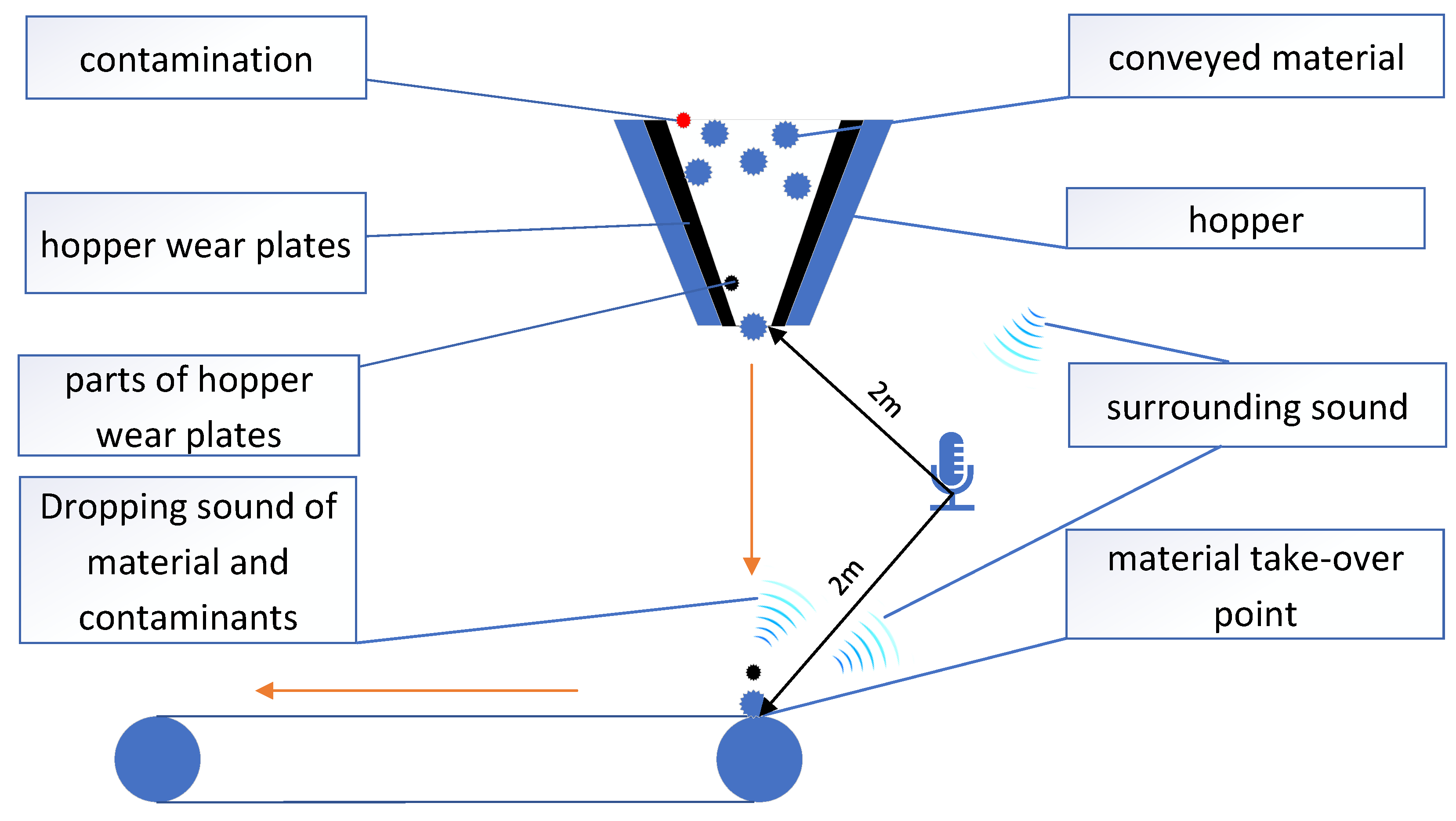
3.1. Measurement Setup

The material is transported over different conveyor belts and stored in hoppers. It is then dispatched to further conveyor belts. In order to reduce wear of the hopper, the hopper is lined with hopper wear plates. As previously mentioned, these wear plates break apart and cause adversarial dropping sound in ongoing transportation. In this research work, the measurement setup consisted of a material hopper for material storage, lined with hopper wear plates and a conveyor belt. The material is dispatched to the conveyor belt at the material take-over point as shown in Figure 1.

The recordings were acquired from a real industrial setting with a microphone placed at a distance of 2 m from the material takeover point and the material hopper. Different sounds such as dropping sound from the material, adversarial dropping sound of contaminants and environmental surrounding sounds were recorded. Environmental surrounding sounds are, for example, caused by conveyor belt noise. The audio sounds were recorded with the Acoustic Expert-hardware device from Primetals Technologies, and its dynamic characteristics are represented in [34].

3.2. Dataset

The dataset was acquired using the previously mentioned measurement setup. In the following, the obtained dataset is summarized through exploratory data analysis. A total of 1030 sequences for five different materials with a length of 10 s were recorded each at a sampling rate of 8 kHz and used for model training and method comparison. Hence, 206 sequences per material class were available for evaluation. In addition to that, a separate robustness test dataset with 100 sequences per material class containing adversarial dropping sound and the material sounds were recorded. The goal of this work is to reliably distinguish between five material classes of different hardness. The five materials with the corresponding Mohs hardness scale are listed in

Table 1. Conveyed Material and their corresponding Mohs hardness scale.

FeSi Br.	FeSi Lumps	Lime	Magnesite	Slag
6.5 [35]	6.5 [35]	3–4 [36]	3.5–4 [37]	5–6 [38]

.

The recordings showed a variability due to different material feed rates, which is seen in Figure 2 from recordings of the same material class.

The respective signal power of the audio dataset in Figure 3 was computed over whole 10 s signal.

In addition to that, the RMS value over the dataset was computed on frames of 25 ms length and the normalized histogram over bins of different RMS values was used in order to compare softer and harder materials. In Figure 4, the histograms for softer and harder materials are illustrated. It was observed that softer materials tend to have lower RMS values around 0.12 and harder materials higher RMS values around 0.2. The distribution of the RMS values for softer materials are Gaussian distributed with a spread of 0.06 and normalized occurance of highest RMS value of about 0.09, where as FeSi and slag have of about 0.13 to 0.24 indicating that the audio signals from softer materials contain characteristic dropping sound with impulses of smaller magnitudes.

The rise time over the whole dataset for characteristic dropping sounds for these materials was computed. The violin-plot of rise times from Figure 5 shows that harder materials have a lower rise time than softer materials, indicating that the impulses of the characteristic sound of harder materials are sharper than softer materials. This is explained because of the more granular and solid consistency of the hard materials.

Based on that, slag, FeSi Br and FeSi Lump contain more characteristic short-term instationarities with high frequencies than magnesite and lime. In Figure 6, the spectrograms for characteristic 10 s recordings for the different materials are shown. The characteristic short-term instationarities are illustrated through the characteristic spread in a frequency range of 1500–2500 Hz, as shown in the first, second and fifth spectrogram of FeSi Br., FeSi Lump and slag from Figure 6.

Based on these findings, it can be confirmed that the acoustic signals of the different materials have specific characteristic patterns for distinguishing between them and are sufficiently represented in the dataset. It was shown that the patterns are not discriminative enough for simple classification. Hence, in the following, a deep-learning-based classification approach is used.

3.3. Audio Frames with Noise

Observations of an audio times-series signal $y\left[n\right]$ consist of a noise-free $x\left[n\right]$ and $v\left[n\right]$ noisy content at the nth sample as defined by

$$y\left[n\right]=x\left[n\right]+v\left[n\right].$$

(1)

To improve the machine learning training and test performance, prior knowledge of the type of disturbances encountered in the described environment will be utilized. The goal is to detect if $y\left[n\right]$ at sample n is corrupted with short-term noise in order to eliminate those signal sections from training and classification. A representative example of an audio recording of a material transport process with a short-term disturbance is shown in Figure 7. Typical disturbances last between 25 and 500 ms. In the next section, the anomaly detector is described in detail.

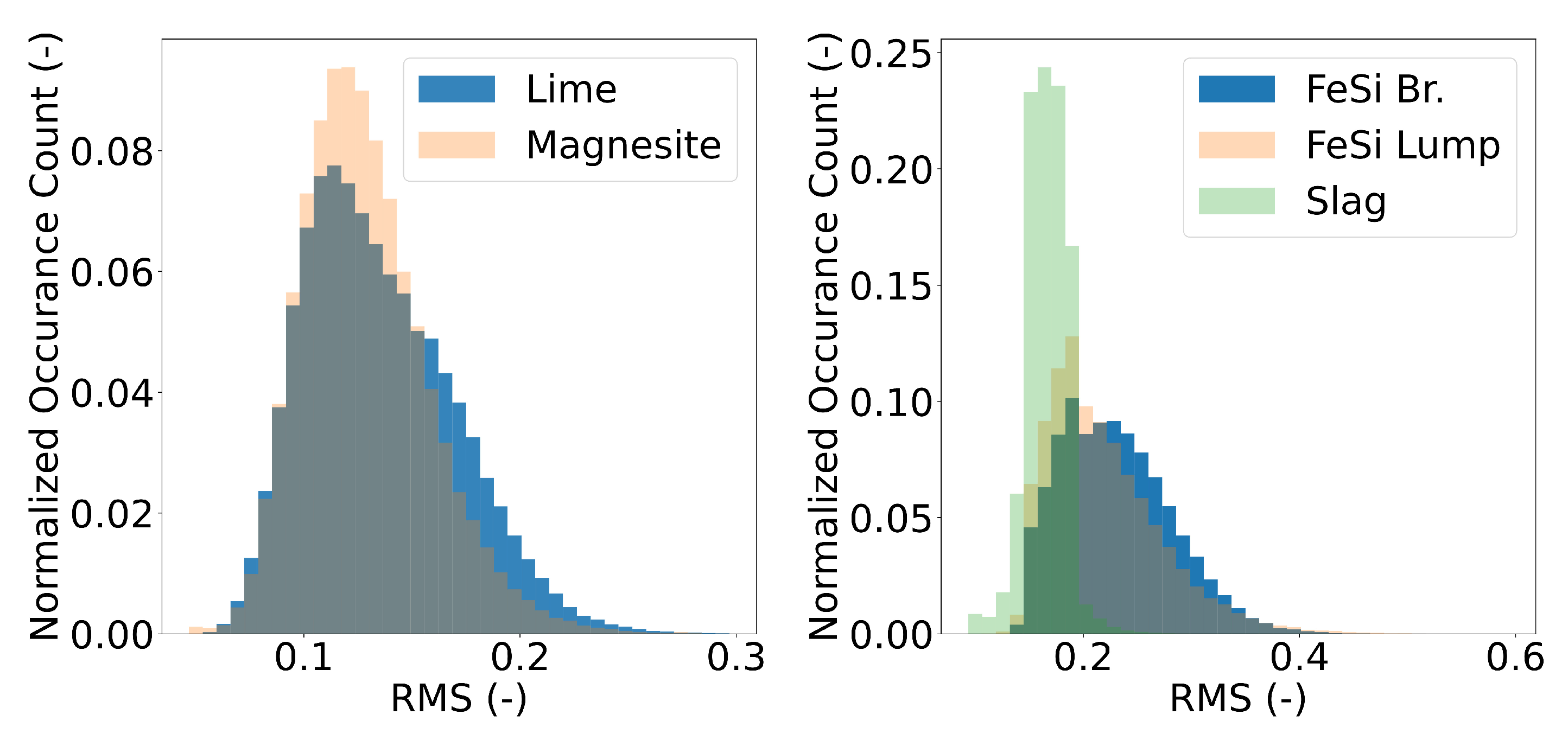
3.3.1. RMSe Outlier Detector

The signal is high pass filtered with a cutoff frequency of 1250 Hz and the short-term RMS is computed with a sliding Blackman window on a frame width of 25 ms length. In the first step, all samples with a RMS value greater than the threshold T as defined in Equation (2) are marked as outliers.

$$T=\alpha ·{\sigma }_y$$

(2)

$\alpha >1$ is defined as the fixed threshold value and ${\sigma }_y$ the standard deviation of the high-pass-filtered 10-s impulse denoised signal. In the second step, the outlier detection signal is extended on the right side of the last detected sample until the RMS value reaches the given level $T_1={\sigma }_y$. If the corresponding distance between two detected impulses is smaller than 400 samples, all in-between samples are marked as outlier samples. Then the detected disturbances are removed. In Figure 8, an example of a sequence of impulses and the detection with RMSe is shown. The peaks at $n=2900$ and $n=3400$ are indicative to the material sound and should therefore remain. The green target line represents the required detection samples.

After detection, the gaps caused by the removal of outlier samples are filled with a frame obtained from uncorrupted sequences of signal $y\left(n\right)$. The uncorrupted sequences from $y\left(n\right)$ are truncated into frames of gap length M. Then, the corresponding RMS value for each frame is computed. The frame with maximum $RMS$ chosen from the uncorrupted N frames of $y\left(n\right)$ is used to fill the gap. Finally, the transitions are crossfaded with 50 samples to prevent abrupt changes between signal subsequences.

3.3.2. Threshold Determination

The selection of the threshold $\alpha$ is a trade-off. As shown in Figure 9, a low $\alpha$ leads to frequent overall restoration yielding to strong removal of informative content of the signal and material class, whereas a high $\alpha$ to low removal of non-characteristic sequences of impulses. The selection of $\alpha$ is done by means of the five-fold cross-validation and classification performance, which is shown later.

4. Classifier

The audio signals from Section 3.2 with a duration of 10 s and an 8 kHz sampling frequency were used for evaluation. For classifier training, algorithm parameter selection and evaluation purposes of the classification neural networks, the audio dataset with 10-s length is validated by means of a five-fold-cross-validation and split into training, validation and model selection test dataset split in proportion of 80%, 10% and 10%, respectively. The classification results are averaged over these five folds. The previously mentioned additional test dataset is used for robustness tests. The experiments were conducted with the TensorFlow v2 framework platform and Python 3.7. The training dataset was preprocessed with previously mentioned anomaly detectors and was used for training the neural network classifier. The audio signals are subdivided into sub-signals and used to obtain the corresponding time-frequency representation. In the following, the applied neural network architectures are presented.

4.1. CNN

As previously mentioned, the audio signals are truncated in sub-signals of equal length and the time–frequency representation is computed. Within this work, BPSD features, as proposed in [6,25], were used as time-frequency representation. BPSD features were computed on a window length of 2048 samples and a hop length of 128 samples. The time–frequency representation serves as an input for a CNN–classifier. Inspired by the model proposed in [5], the deep learning model applied within this paper consists of different types of layers, which are merged into the final predicting model. As shown in

Table 2. CNN-architecture.

Name	Type	Kernel /Filter/Stride Size	Pooling Size	Dropout Rate	Output Activation Function
L1	Conv2D	k × k/48/1 × 1			ReLu
L2	Max Pooling		4 × 4
L3	Dropout			0.5
L4	Conv2D	k × k/48/1 × 1			ReLu
L5	Max Pooling		4 × 4
L6	Dropout			0.4
L7	Conv2D	k × k/96/1 × 1			ReLu
L8	Flatten				ReLu
L9	Dropout			0.5
L10	Dense	64
L11	Dense	5			softmax

, two convolutional layers with 48 filters serve for feature extraction. Different kernel widths $k=[3,5,7]$ and number of frequency bins were used to obtain the most appropriate combination. Pooling layers are used for feature reduction and therefore provide a mapping function to lower dimensions [5]. A dropout rate of 0.4 and 0.5 was used to reduce overfitting. Finally, another convolution layer, a fully connected layer with 64 hidden units as in [5] and a softmax layer are applied for obtaining the probability scores of the CNN.

Between the convolutional layers, the ReLu-activation function was used. The weights were initialized with the He-Weight Initialization strategy and a training batch size of 32 1-s samples was chosen. The training was done over 100 epochs. For training the cross-categorical loss function and Adam update rule were used. The initial learning rate was set to ${10}^{-3}$ with learning rate decays ${\beta }_1=0.9$ and ${\beta }_2=0.999$. The batch size, initial learning rate and initial learning rate decays were chosen by applying a grid search and overall averaged classification accuracy on the validation dataset splits as proposed in [39]. In order to reduce the effect of overfitting and overtraining, early stopping and no-improvement after 10 epochs were applied. In the first step, the previously mentioned CNN-structure was compared using different frequency bins $n_{bins}=[24,128,512]$, 1 s input window length as in [6,25] and kernel widths $k=[3,5,7]$. The comparison was done by means of the overall classification accuracy on five-fold-cross-validation, averaged over the different validation dataset splits. For CNN selection, the training dataset was not processed and the frequency range of 50–3.5 kHz was used because the majority of the surrounding sound like conveyor belt and other environmental sounds are out of these frequency range. In Figure 10 it can be observed that the worst results for all frequency bin configurations were achieved with $k=3$ and $k=7$. The best results were achieved with a configuration of $n_{bins}=128$ and $k=5$. Hence, this configuration was subsequently used.

In a second step, the input window lengths w for the CNN were varied and the previously mentioned CNN architecture was used. A 10-s sequence was split in equally-sized frames of 5 s, 2 s, 1 s or 500 ms length, resulting in 2, 5, 10 or 20 frames per sequence. From these frames an input representation for the CNN containing 128 frequency bins and 305, 122, 61 or 30 time bins was computed. The training batch sizes for the different input window lengths were found with Grid Search and batch sizes of $[8,16,32,64]$ for $w=[5\mathrm{s},2\mathrm{s},1\mathrm{s},500\mathrm{ms}]$ input window lengths were used. Due to the given process constraint that for every 10 s a final decision is required, majority voting was applied. In Figure 11, the achieved results on the validation dataset without and with majority voting are shown. It can be observed that majority voting improved overall results for every configuration. Best results with less tendency of overfitting were achieved with a 1-s configuration. Hence, this configuration is further used for evaluation. In Figure 12 the final classifier structure is shown.

In a final step, the training and validation dataset is preprocessed with different $\alpha =[1.5,1.625,1.75]$ and the overall classification results of the proposed CNN on the validation dataset were compared as shown in Figure 13. Best results with $\alpha =1.625$ were found, which was subsequently used. For $\alpha =1.5$ remarkable amount of informative content from the training dataset was removed. $\alpha =1.75$ yielded that non-characteristic instationarities remained in the dataset.

4.2. FF-NN

The proposed FF-NN-architecture from [6] was used to compare with the performance of CNN. FF-NN was trained using the same dataset as CNN. The same hyperparameters as in [6] were applied. In the next chapter, the FF-NN is compared to the CNN-classifier.

5. Results

In this section, the previously mentioned CNN and FF-NN were compared. In addition, the impact of preprocessing is illustrated. Finally, this chapter is concluded with a robustness test.

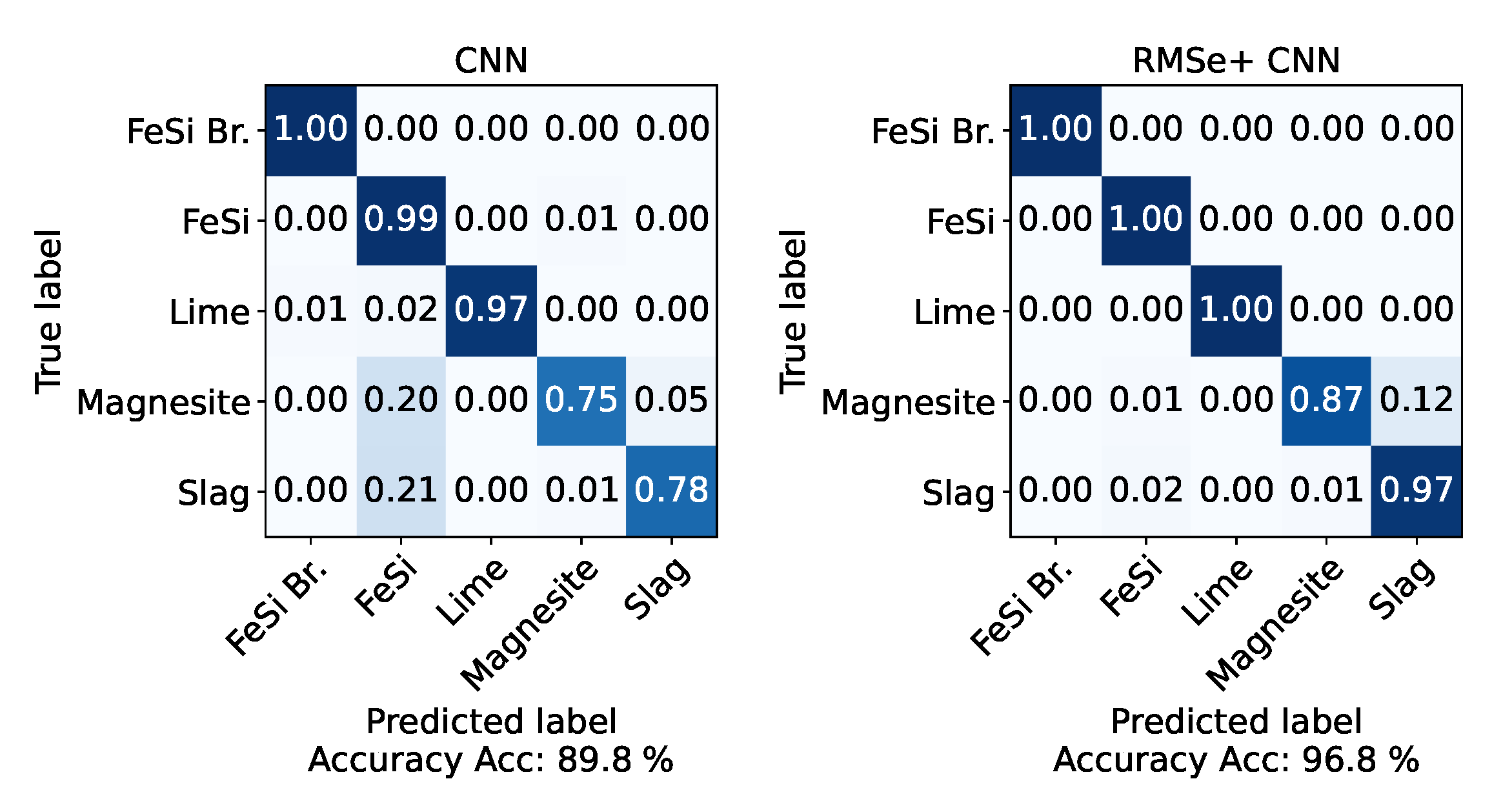
5.1. Model Comparison

Previously mentioned training and validation dataset splits were used for training with RMSe-preprocessed data. This model is applied to the model comparison test dataset and the test is repeated five times with different 10-s audio signals. The achieved results for both neural networks are reported in Figure 14. We observed for FF-NN a performance improvement for RMSe preprocessed training data. For the FF-NN, the overall classification results improved from 96.2% to 96.8% for RMSe preprocessed dataset. The classification results for CNN improved from 97% to 98% respectively. The RMSe applied to the training dataset reached better results on the cost of biasing towards material class slag. The misclassification between FeSi Lump and magnesite was reduced to 3%. We observed an improvement in the classification performance of magnesite and slag with CNN and a reduction of maximum misclassification from 7% to 4%. It was observed that CNN trained on RMSe preprocessed dataset achieved best results, indicating that the CNN was able to learn more discriminative features. Therefore, this combination is used for robustness tests.

5.2. Robustness Test

Previously, CNN-architecture trained on the preprocessed dataset was used to assess the performance on a heavily contaminated robustness test dataset containing anomalies from adversarial dropping sounds of contaminants. The anomaly widths varied from 250 ms to 500 ms. Within each of the 10-s sequences from this dataset, containing 10 frames with 1 s length, the anomalies occurred in six out of ten frames. In Figure 15 the achieved results are shown. It can be observed, that the CNN is sensitive to impulse noise. A performance of 89.8% is reached. The significant misclassification between residual material slag towards materials with higher hardness like FeSi and FeSi Br is noticed. On the other hand, preprocessing with RMSe improved the results in 96.8% overall accuracy and a decrease of misclassification between materials. The misclassification of slag with other materials such as magnesite was still observed. This is explained with the fact that slag is a residual material obtained within the steelmaking process and its chemical consistency can differ. Traces of other materials such as magnesite may be present.

6. Conclusions

In this paper, a deep-learning-based classification system for material transport in steelmaking was introduced. It was observed that impulse noise caused by dropping sounds of contaminants such as hopper wear plates affects the overall classification performance. Hence, anomaly detection based on RMSe was used. Furthermore, a CNN-based material-type classification algorithm was compared with an FF-NN-classification algorithm. It was observed that the introduced CNN architecture gave significantly better performance than FF-NN, indicating that more discriminative features were learned. In addition to that, supplementary robustness tests indicated that the impulse noise increased the misclassification of residual material towards materials with higher hardness. The RMSe-preprocessing led to robustness increase. On this basis, we conclude that outlier detection and preprocessing have a significant contribution to improving overall classification results and robustness, which is crucial for acoustic material monitoring in harsh steel industrial environments. In the current study, the RMSe did not use information from the frequencies. Hence, further research on outlier detection methods with the inclusion of both temporal and frequency features might become a promising way towards the detection of other occurring outlier events within acoustic monitoring in steelplants.

References

1. Johannes. Update-Fehler verursachte Russ-Ausstoss der Dillinger Huette. Saarbruecker Ztg. 2018, 9, 5–7. [Google Scholar]
2. Berckmans, D.; Janssens, K.; Van der Auweraer, H.; Sas, P.; Desmet, W. Model-based synthesis of aircraft noise to quantify human perception of sound quality and annoyance. J. Sound Vib. 2008, 311, 1175–1195. [Google Scholar] [CrossRef]
3. Ding, R.; Pang, C.; Liu, H. Audio-Visual Keyword Spotting Based on Multidimensional Convolutional Neural Network. In Proceedings of the 2018 25th IEEE International Conference on Image Processing (ICIP), Athens, Greece, 7–10 October 2018; pp. 4138–4142. [Google Scholar] [CrossRef]
4. Serizel, R.; Bisot, V.; Essid, S.; Richard, G. Acoustic Features for Environmental Sound Analysis. In Computational Analysis of Sound Scenes and Events; Virtanen, T., Plumbley, M.D., Ellis, D., Eds.; Springer International Publishing: Cham, Switzerland, 2018; pp. 71–101. [Google Scholar] [CrossRef] [Green Version]
5. Salamon, J.; Bello, J.P. Deep Convolutional Neural Networks and Data Augmentation for Environmental Sound Classification. IEEE Signal Process. Lett. 2017, 24, 279–283. [Google Scholar] [CrossRef]
6. Husaković, A.; Pfann, E.; Huemer, M. Robust Machine Learning Based Acoustic Classification of a Material Transport Process. In Proceedings of the 2018 14th Symposium on Neural Networks and Applications (NEUREL), Belgrade, Serbia, 20–21 November 2018; pp. 1–4. [Google Scholar] [CrossRef]
7. Valenti, M.; Squartini, S.; Diment, A.; Parascandolo, G.; Virtanen, T. A convolutional neural network approach for acoustic scene classification. In Proceedings of the 2017 International Joint Conference on Neural Networks (IJCNN), Anchorage, AK, USA, 14–19 May 2017; pp. 1547–1554. [Google Scholar] [CrossRef]
8. Nystuen, J.A. Listening to Raindrops; Solstice: An Electronic Journal of Geography and Mathematics; Institute of Mathematical Geography: Ann Arbor, MI, USA, 1999. [Google Scholar]
9. Ramona, M.; Peeters, G. AudioPrint: An efficient audio fingerprint system based on a novel cost-less synchronization scheme. In Proceedings of the 2013 IEEE International Conference on Acoustics, Speech and Signal Processing, Vancouver, BC, Canada, 26–31 May 2013; pp. 818–822. [Google Scholar]
10. Velankar, M.; Kulkarni, P. Music Recommendation Systems: Overview and Challenges. In Advances in Speech and Music Technology; Springer: Berlin/Heidelberg, Germany, 2023; pp. 51–69. [Google Scholar]
11. Andraju, L.B.; Raju, G. Damage characterization of CFRP laminates using acoustic emission and digital image correlation: Clustering, damage identification and classification. Eng. Fract. Mech. 2023, 277, 108993. [Google Scholar] [CrossRef]
12. Dong, L.; Zhang, Y.; Bi, S.; Ma, J.; Yan, Y.; Cao, H. Uncertainty investigation for the classification of rock micro-fracture types using acoustic emission parameters. Int. J. Rock Mech. Min. Sci. 2023, 162, 105292. [Google Scholar] [CrossRef]
13. Yu, A.; Liu, X.; Fu, F.; Chen, X.; Zhang, Y. Acoustic Emission Signal Denoising of Bridge Structures Using SOM Neural Network Machine Learning. J. Perform. Constr. Facil. 2023, 37, 04022066. [Google Scholar] [CrossRef]
14. Temko, A.; Nadeu, C. Classification of acoustic events using SVM-based clustering schemes. Pattern Recognit. 2006, 39, 682–694. [Google Scholar] [CrossRef]
15. Šmak, R.; Votava, J.; Lozrt, J.; Kumbár, V.; Binar, T.; Polcar, A. Analysis of the Degradation of Pearlitic Steel Mechanical Properties Depending on the Stability of the Structural Phases. Materials 2023, 16, 518. [Google Scholar] [CrossRef] [PubMed]
16. Uher, M.; Beneš, P. Measurement of particle size distribution by the use of acoustic emission method. In Proceedings of the 2012 IEEE International Instrumentation and Measurement Technology Conference Proceedings, Graz, Austria, 13–16 May 2012; pp. 1194–1198. [Google Scholar] [CrossRef]
17. Taheri, H.; Koester, L.W.; Bigelow, T.A.; Faierson, E.J.; Bond, L.J. In situ additive manufacturing process monitoring with an acoustic technique: Clustering performance evaluation using K-means algorithm. J. Manuf. Sci. Eng. 2019, 141, 041011. [Google Scholar] [CrossRef]
18. Tieghi, L.; Becker, S.; Corsini, A.; Delibra, G.; Schoder, S.; Czwielong, F. Machine-learning clustering methods applied to detection of noise sources in low-speed axial fan. J. Eng. Gas Turbines Power 2023, 145, 031020. [Google Scholar] [CrossRef]
19. Liu, B.; Liu, C.; Zhou, Y.; Wang, D.; Dun, Y. An unsupervised chatter detection method based on AE and merging GMM and K-means. Mech. Syst. Signal Process. 2023, 186, 109861. [Google Scholar] [CrossRef]
20. Hayashi, T.; Yoshimura, T.; Adachi, Y. Conformer-Based Id-Aware Autoencoder for Unsupervised Anomalous Sound Detection. DCASE2020 Challenge; Technical Report. 2020. Available online: https://dcase.community/documents/challenge2020/technical_reports/DCASE2020_Hayashi_111_t2.pdf (accessed on 23 December 2022).
21. Li, W.; Parkin, R.M.; Coy, J.; Gu, F. Acoustic based condition monitoring of a diesel engine using self-organising map networks. Appl. Acoust. 2002, 63, 699–711. [Google Scholar] [CrossRef]
22. Barchiesi, D.; Giannoulis, D.; Stowell, D.; Plumbley, M.D. Acoustic Scene Classification: Classifying environments from the sounds they produce. IEEE Signal Process. Mag. 2015, 32, 16–34. [Google Scholar] [CrossRef]
23. Chachada, S.; Kuo, C.C.J. Environmental sound recognition: A survey. In Proceedings of the 2013 Asia-Pacific Signal and Information Processing Association Annual Summit and Conference, Kaohsiung, Taiwan, 29 October–1 November 2013; pp. 1–9. [Google Scholar] [CrossRef]
24. Su, F.; Yang, L.; Lu, T.; Wang, G. Environmental Sound Classification for Scene Recognition Using Local Discriminant Bases and HMM. In Proceedings of the 19th ACM International Conference on Multimedia, MM ’11, Scottsdale, AZ, USA, 28 November–1 December 2011; Association for Computing Machinery: New York, NY, USA, 2011; pp. 1389–1392. [Google Scholar] [CrossRef]
25. Husaković, A.; Mayrhofer, A.; Pfann, E.; Huemer, M.; Gaich, A.; Kühas, T. Acoustic Monitoring—A Deep LSTM Approach for a Material Transport Process. In Proceedings of the Computer Aided Systems Theory—EUROCAST 2019: 17th International Conference, Las Palmas de Gran Canaria, Spain, 17–22 February 2019; Revised Selected Papers, Part II. Springer: Berlin/Heidelberg, Germany, 2019; pp. 44–51. [Google Scholar] [CrossRef]
26. Tagawa, Y.; Maskeliūnas, R.; Damaševičius, R. Acoustic Anomaly Detection of Mechanical Failures in Noisy Real-Life Factory Environments. Electronics 2021, 10, 2329. [Google Scholar] [CrossRef]
27. Oudre, L. Automatic Detection and Removal of Impulsive Noise in Audio Signals. Image Process. Line 2015, 5, 267–281. [Google Scholar] [CrossRef] [Green Version]
28. Zhou, C.; Paffenroth, R.C. Anomaly Detection with Robust Deep Autoencoders. In Proceedings of the 23rd ACM SIGKDD International Conference on Knowledge Discovery and Data Mining, KDD ’17, Halifax, NS, Canada, 13–17 August 2017; Association for Computing Machinery: New York, NY, USA, 2017; pp. 665–674. [Google Scholar] [CrossRef]
29. Malhotra, P.; Vig, L.; Shroff, G.; Agarwal, P. Long Short Term Memory Networks for Anomaly Detection in Time Series. ESANN 2015, 2015, 89. [Google Scholar]
30. Wang, Y.; Zheng, Y.; Zhang, Y.; Xie, Y.; Xu, S.; Hu, Y.; He, L. Unsupervised Anomalous Sound Detection for Machine Condition Monitoring Using Classification-Based Methods. Appl. Sci. 2021, 11, 11128. [Google Scholar] [CrossRef]
31. Blázquez-García, A.; Conde, A.; Mori, U.; Lozano, J.A. A Review on Outlier/Anomaly Detection in Time Series Data. ACM Comput. Surv. 2021, 54, 1–33. [Google Scholar] [CrossRef]
32. Aggarwal, C.C. Probabilistic and Statistical Models for Outlier Detection. In Outlier Analysis; Springer International Publishing: Cham, Switzerland, 2017; pp. 35–64. [Google Scholar] [CrossRef]
33. Kasparis, T.; Lane, J. Adaptive scratch noise filtering. IEEE Trans. Consum. Electron. 1993, 39, 917–922. [Google Scholar] [CrossRef]
34. Hartl, F.; Mayrhofer, A.; Rohrhofer, A.; Stohl, K. Off the Beaten Path: New Condition Monitoring Applications in Steel Making. In Proceedings of the 3rd European Steel Technology and Application Days—ESTAD 2017, Vienna, Austria, 26–29 June 2017; Austrian Society for Metallurgy and Materials (ASMET): Vienna, Austria, 2017; pp. 44–51. [Google Scholar]
35. Nicheng, S.; Wenji, B.; Guowu, L.; Ming, X.; Jingsu, Y.; Zhesheng, M.; He, R. Naquite, FeSi, a New Mineral Species from Luobusha, Tibet, Western China. Acta Geol. Sin. Engl. Ed. 2012, 86, 533–538. [Google Scholar] [CrossRef]
36. Watkins, K.W. Lime. J. Chem. Educ. 1983, 60, 60. [Google Scholar] [CrossRef]
37. Shanmugasundaram, V.; Shanmugam, B. Characterisation of magnesite mine tailings as a construction material. Environ. Sci. Pollut. Res. 2021, 28, 45557–45570. [Google Scholar] [CrossRef] [PubMed]
38. Smith, K.; Morian, D. Use of Air-cooled Blast Furnace Slag as Coarse Aggregate in Concrete Pavements: A Guide to Best Practise. Fed. Highw. Adm.-Tech Rep. 2012, 6, 8. [Google Scholar]
39. Bergstra, J.; Bardenet, R.; Bengio, Y.; Kégl, B. Algorithms for hyper-parameter optimization. In Proceedings of the 25th Annual Conference on Neural Information Processing Systems, Granada, Spain, 12–15 December 2011; p. hal-00642998f. [Google Scholar]
Figure 1. Measurement setup consisting of conveyor belt and material hopper (distances are colored in black, material flow in orange).
Applsci 13 01843 g001
Figure 2. Different feed rates for same material class.
Applsci 13 01843 g002
Figure 3. Variability of the dataset: Different material feed rates and classes.
Applsci 13 01843 g003
Figure 4. RMS of the dataset computed on frames of 25 ms width: (left) softer materials and (right) harder materials.
Applsci 13 01843 g004
Figure 5. Rise times of characteristic dropping sound for different materials.
Applsci 13 01843 g005
Figure 6. Spectrograms of typical audio signals for different material classes of length 10 s and window width h = 2048 .
Applsci 13 01843 g006
Figure 7. An example of an audio recording corrupted with impulse noise (red).
Applsci 13 01843 g007
Figure 8. RMSe detectors applied on sequences of impulses.
Applsci 13 01843 g008
Figure 9. RMSe-algorithm applied on training dataset: (left) histogram of anomaly duration and (right) overall restoration content of training dataset.
Applsci 13 01843 g009
Figure 10. Accuracy with different kernel widths k and frequency bins n b i n s achieved on the validation data splits of 5-fold cross-validation.
Applsci 13 01843 g010
Figure 11. Accuracy with different window lengths w with and without majority voting achieved on a 5 fold cross validation.
Applsci 13 01843 g011
Figure 12. Final classifier consisting of 10 CNNs and majority voting.
Applsci 13 01843 g012
Figure 13. CNN-Accuracy with different thresholds α achieved on 5-fold cross-validation and validation dataset splits.
Applsci 13 01843 g013
Figure 14. Achieved classification performance and confusion matrixes (from left to right) on test dataset splits: first row: FF-NN without preprocessing, FF-NN trained on RMSe preprocessed dataset second row: CNN without preprocessing, CNN trained on RMSe preprocessed dataset.
Applsci 13 01843 g014
Figure 15. Achieved classification performance and confusion matrixes on robustness test dataset: CNN (left) and CNN with RMSe preprocessing (right).
Applsci 13 01843 g015