Article

Short-Term Power Prediction of Wind Turbine Applying Machine Learning and Digital Filter

School of Energy and Power Engineering, Lanzhou University of Technology, Lanzhou 730050, China
*
Authors to whom correspondence should be addressed.
Appl. Sci. 2023, 13(3), 1751; https://doi.org/10.3390/app13031751
Submission received: 7 January 2023 / Revised: 21 January 2023 / Accepted: 27 January 2023 / Published: 30 January 2023
(This article belongs to the Section Energy Science and Technology)

Abstract

:
As wind energy development increases, accurate wind energy forecasting helps to develop sensible power generation plans and ensure a balance between supply and demand. Machine-learning-based forecasting models possess exceptional predictive capabilities, and data manipulation prior to model training is also a key focus of this research. This study trained a deep Long Short-Term Memory (LSTM) neural network to learn the processing results of the Savitzky-Golay filter, which can avoid overfitting due to fluctuations and noise in measurements, improving the generalization performance. The optimum data frame length to match the second-order filter was determined by comparison. In a single-step prediction, the method reduced the root-mean-square error by 3.8% compared to the model trained directly with the measurements. The method also produced the smallest errors in all steps of the multi-step advance prediction. The proposed method ensures the accuracy of the forecasting and, on that basis, also improves the timeliness of the effective forecasts.

1. Introduction

The large-scale development and utilization of new energy is conducive to the smooth realization of low-carbon goals. According to the “bp Statistical Review of World Energy 2022” [1], benefiting from the strong growth of wind and solar energy, renewable energy accounts for 12.8% of the total global energy use in 2021, surpassing nuclear energy, which accounts for 9.8%; renewable energy power generation increased by 16.5% compared to the previous year, while coal power generation increased by only 8.5%, and natural gas power generation increased by only 2.3%. In the process of promoting the development and utilization of unstable energy such as wind energy and solar energy, the imbalance of supply and demand caused by its intermittent nature is a major threat to the safe and stable operation of the power transmission and transformation network [2]. In order to improve the energy network’s ability to absorb renewable energy, a feasible method is to predict and evaluate uncertain renewable energy, and then improve the resilience of the energy system through joint complementary means such as storage conversion [3], demand-side management [4], and co-ordination of electric vehicle charging needs [5]. The reasonable planning of equipment capacity parameters and formulation of production scheduling plans on the basis of prediction and evaluation can further reduce operating costs.
According to different time scales, the current forecasting methods can be divided into ultra-short-term forecasting [6,7], short-term forecasting [8], medium-term, and long-term forecasting [9,10]. The prediction method models mainly include the physical model [11,12], statistical model [13], grey model [14,15], and machine learning [16,17]. Among them, the physical model builds and solves the atmospheric flow equations; the statistical model uses differential equations to solve the trend of data correlation; and the artificial intelligence method [18] which is good at dealing with multi-dimensional nonlinear problems is increasingly being used to break through computational bottlenecks of traditional methods. Improving forecast accuracy is one of the research focuses on issues related to renewable energy forecasting. Data feature enhancement and model algorithm optimization are currently widely used ideas. In the data pre-processing analysis stage, variable correlations or priorities are calculated to extract relevant feature parameters [19,20]. Periodic fluctuation features are then separated by data stacking [21] or modal decomposition [22,23,24] or discrete wavelet transform [25], which can achieve the goal of improving prediction accuracy. Deep learning or neural networks are widely chosen for building novel predictive models with complex structures. For example, a model combined with a graph-structured neural network [26] can better identify the spatial correlation of data, and a model based on a long-short-term memory neural network [27] can learn the temporal correlation of data well. As the structure of the emerging model becomes complex and diverse, a large number of internal parameters are globally adjusted by the excellent optimizer [28,29,30] to achieve the overall best working performance. On the premise of ensuring the accuracy of the prediction, the calculation amount of the network parameter optimization can be reduced by means of an optimized weight calculation [31] and attention mechanism [6,32], so that the model calculation performance can be improved.
It is worth noting that the development of artificial intelligence has brought new ideas to the field of energy research. Machine learning is a powerful tool for data mining that can be flexibly extended and combined to perform data-related tasks, and wind power prediction based on it has received a great deal of attention in the energy field.
In this study, machine learning was used in order to achieve accurate wind energy prediction. Deep Long Short-Term Memory (LSTM) neural network was created, and in particular we also focused on the processing of the data’s own features. Due to the power of machine-learning models, the processing of the data itself is often ignored. The main contributions are the following:
  • The output of the training set was optimized by a Savitzky-Golay filter, and the deep LSTM network trained by this reduced overfitting and exhibited better generalization performance.
  • The optimal configuration parameters of the digital filter were determined. With such a configuration, the noise can be filtered out well and the original features retained, and the prediction model will not be overfitted due to the learned noise.
  • More accurate multi-step predictions were achieved based on machine learning and digital filtering, which can improve the timeliness of the prediction information.
The content of the article is organized as follows: The content of Section 2 is about the basic concepts of the methods and models used. Section 3 is about data presentation and comparative analysis in practical analytical calculation cases. Section 4 summarizes all the content and gives the conclusion.

2. Methodology Model

2.1. Overall Data Flow

For the wind turbine short-term ahead power prediction problem designed in this study, the prediction process established is shown in Figure 1. The Supervisory Control and Data Acquisition (SCADA) data of the wind turbine was first acquired and then the raw data was pre-processed by digital filter for noise reduction. Next, the dataset pre-processing process for the supervised learning task was executed, and on the basis of this work, we will be able to implement the prediction of continuous time series. The final predictor was the LSTM neural network, but of course several other machine-learning methods were also used as predictors in this session to test the effect. With this complete set of processes, the short-term power output prediction of wind turbine can be effectively implemented.

2.2. Digital Filter

The data of wind speed measured in real conditions contains a lot of noise that can affect the learning of the model, so it is necessary to process the noise to enhance the data quality. In this study, the digital filter Savitzky-Golay (SG) filter was applied to enhance the accuracy of the data signal by subtracting noise.
SG filter is a type of Finite Impulse Response (FIR) digital filter; it achieves noise reduction by convolution operations on the data frames. The relative extremes and width distribution of the original sequence should be preserved when using it. SG filter has two critical degrees of freedom [33], polynomial order and data frame length. With the flexible adjustment of these two degrees of freedom, the SG filter can perform its excellent performance in many signal-processing scenarios. Considering these advantages, the SG filter was adopted in this study.
SG filter operates by local least squares approximation fitting to filter the noise signal [34]. The local polynomial is expressed as follows, with a data frame containing a total of 2M +1 sample points centered at n = 0:
p ( n ) = k = 0 N a k n k
where N ( N 2 M + 1 ) is the power of the polynomial.
In order to find the desired polynomial result, the error between the estimated and original values is evaluated to minimize it, and the error is calculated by the following equation:
ε N = n = M M p ( n ) x [ n ] 2 = n = M M k = 0 N a k n k x [ n ] 2
The output of the filter can be represented by a discrete convolution of the following form:
y [ n ] = m = M M h [ m ] x [ n m ] = m = n M n + M h [ n m ] x [ m ]

2.3. Method of Prediction

2.3.1. Neural Network Units

The unique feedback loop structure of Recurrent Neural Network (RNN) can realize the cyclic update of data, so as to realize the time memory function. The time-unfolded computational graph of RNN is shown in Figure 2. The following update equations are applied:
a ( t ) = b + W h ( t 1 ) + U x ( t )
h ( t ) = tan h ( a ( t ) )
o ( t ) = c + V h ( t )
The parameters are the bias vectors b and c along with the weight matrices U, V, and W, respectively, for input-to-hidden, hidden-to-output, and hidden-to-hidden connections.
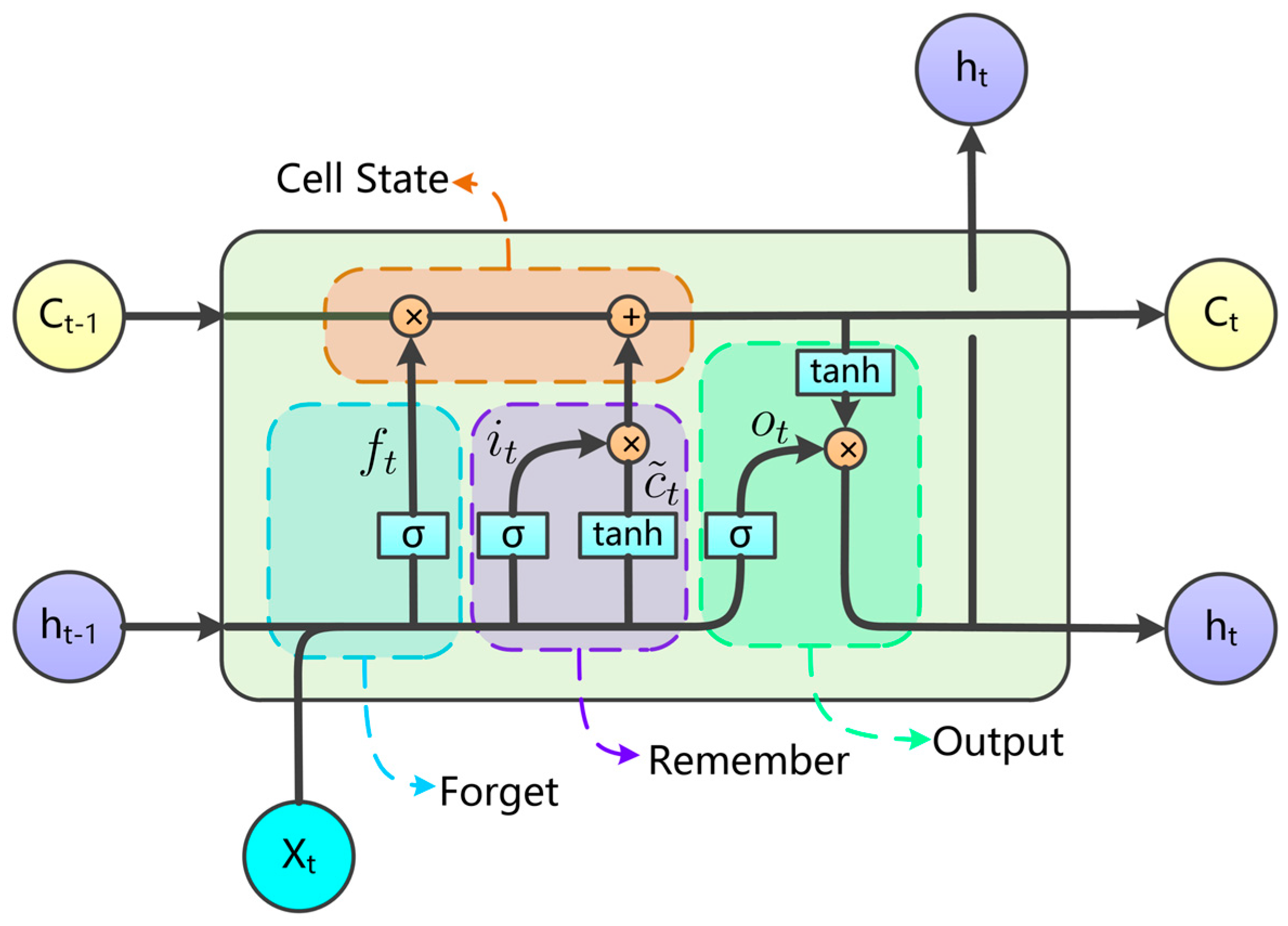
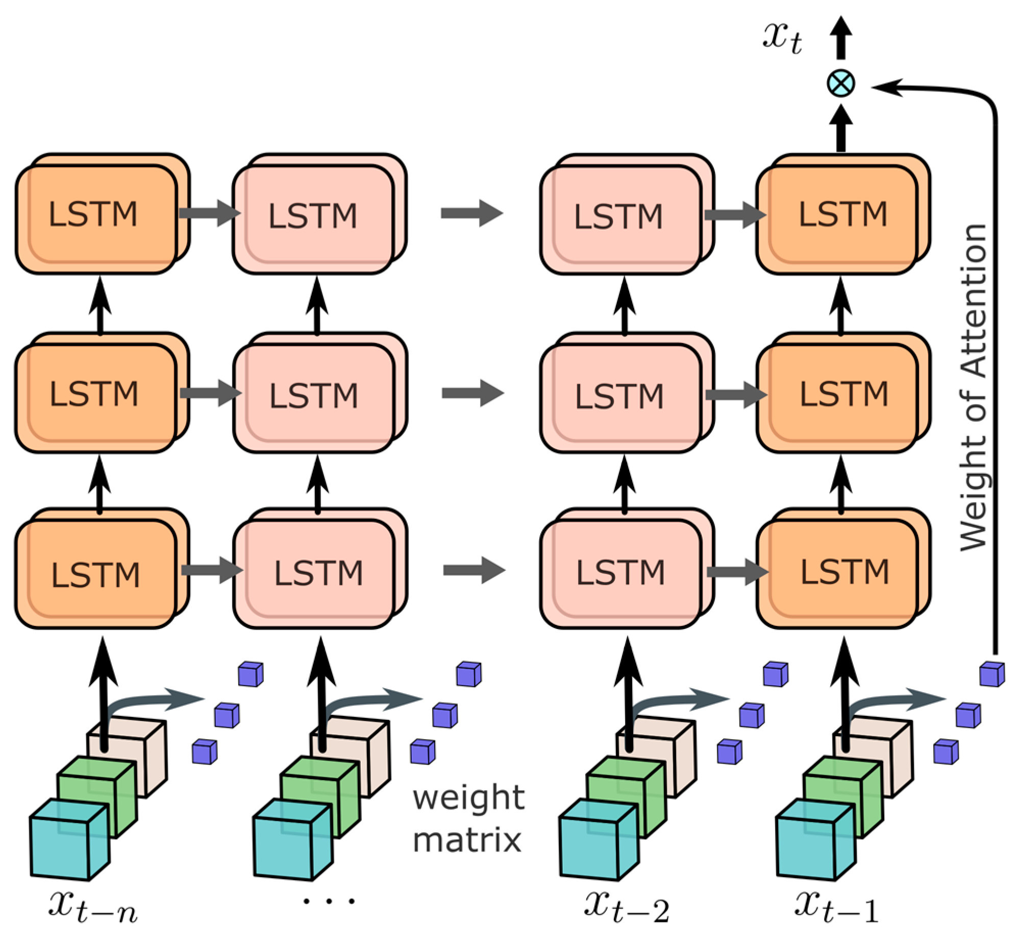
Sequence information that is too long is difficult for RNN to process. To solve this problem, the LSTM neural network introduces a separate memory unit c t to retain historical information, and controls the information flow in the learning process through the forgetting gate, input gate, and output gate. Its structure is shown in Figure 3. Therefore, LSTM can selectively forget, delete, or update the internal information of the network, so as to achieve a better learning effect on the long-term dependence of the information in the sequence [35]. The compact forms of the equations for an LSTM cell are:
f t = σ g ( W f x t + U f h t 1 + b f )
i t = σ g ( W i x t + U i h t 1 + b i )
o t = σ g ( W o x t + U o h t 1 + b o )
c ˜ t = σ c ( W c x t + U c h t 1 + b c )
c t = f t c t 1 + i t c ˜ t
h t = o t σ h ( c t )
where x t is the input vector; and f t , i t , and o t indicate the activation vector of forget gate, input gate, and output gate, respectively. h t indicates the hidden state vector also known as output vector of the LSTM unit. c ˜ t indicates cell input activation vector. c t indicates cell state vector. σ denotes the activation function of the gate (normally sigmoid function and hyperbolic tangent function). W, U, and b are weight matrices and bias vector parameters which need to be learned during training. The operator (Hadamard product) denotes the element-wise multiplication of elements between two vectors.

2.3.2. Time Series Forecasting to Supervised Learning

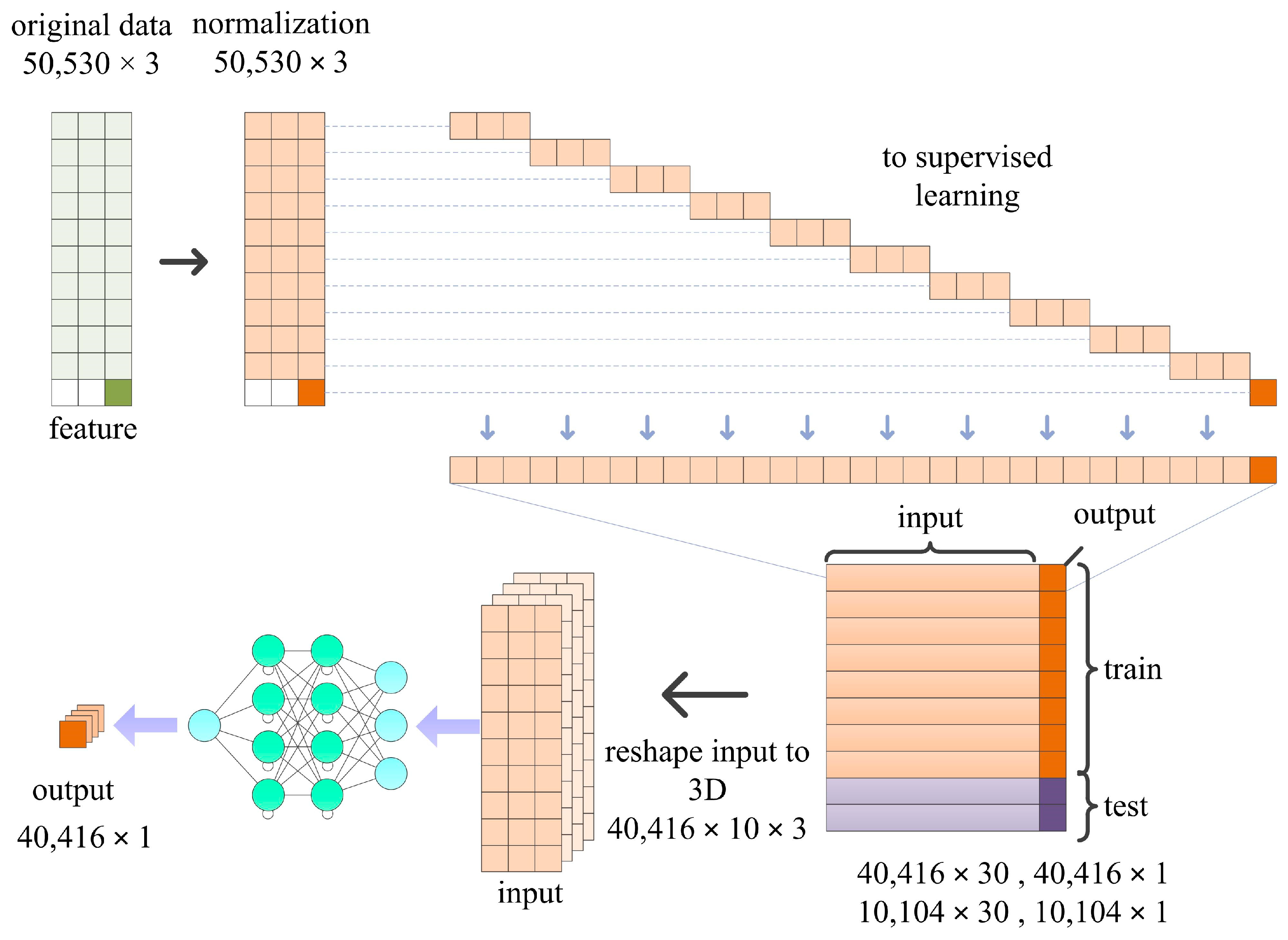
The main steps to train a deep learning model for wind power prediction are as follows: Firstly, data cleaning is performed on the SCADA data of wind turbines, and multi-dimensional feature variables are normalized. Then, the normalized data is transformed into a supervised learning dataset, divided into a training set and a test set, and transformed into a standard matrix format specified by the model. Then, we define the model input and output parameters and nodes. Finally, the data of the training set is used to train the model to get the best threshold and weight parameters, and the test set is used to test the prediction accuracy of the model. The framework of the above supervised learning process is shown in Figure 4.

3. Time Series Forecasting Experiments

3.1. Data Description

3.1.1. General Overview

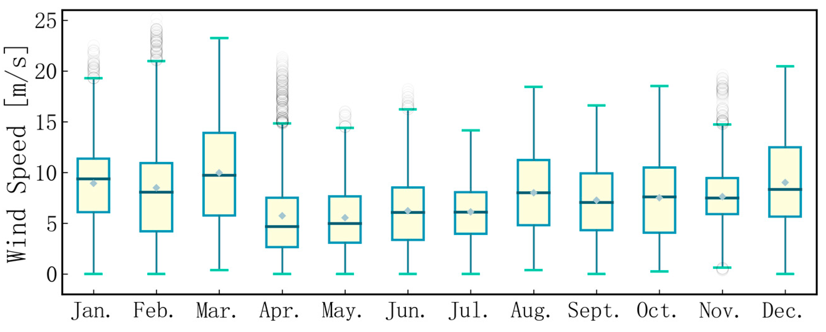
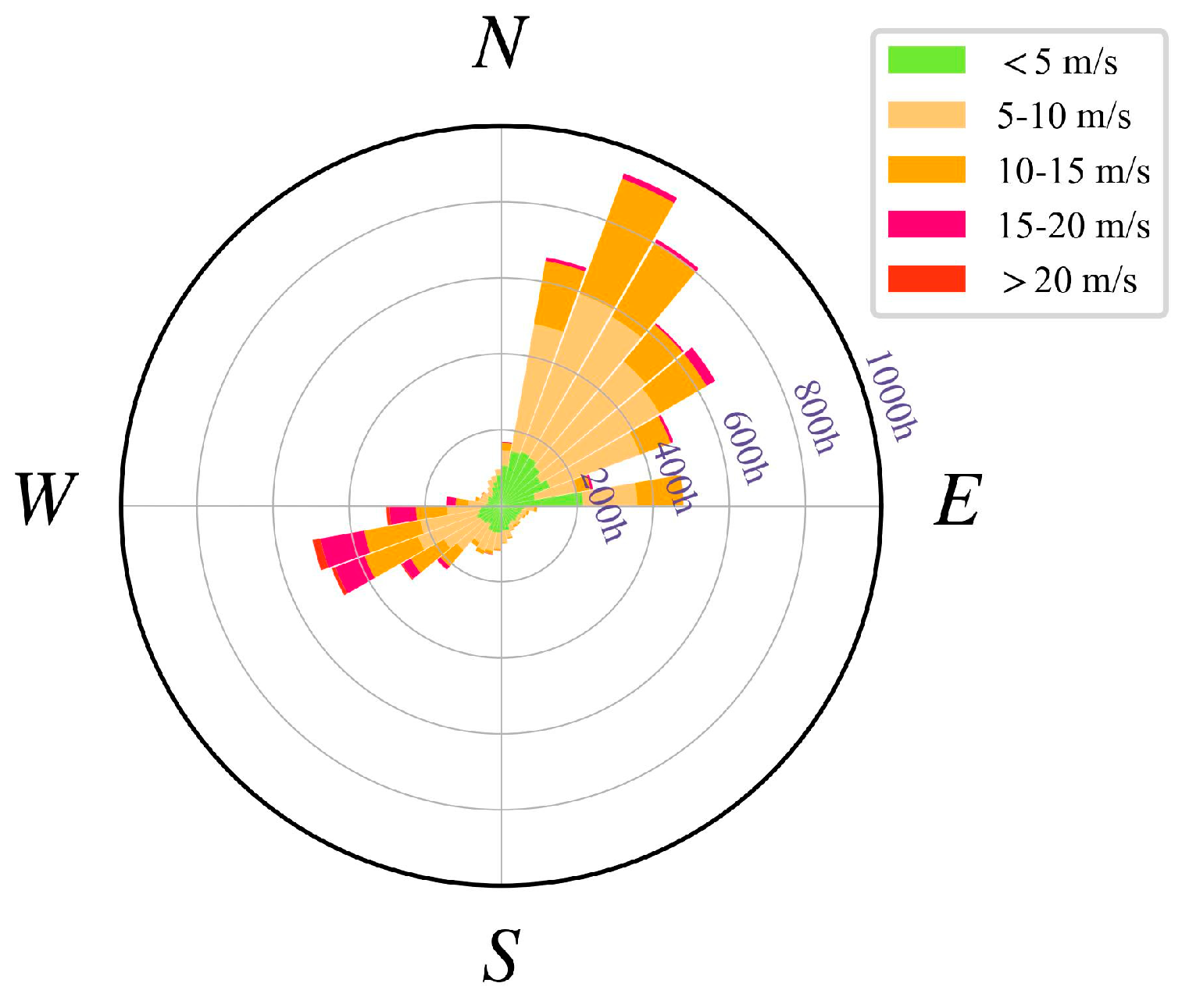
The data comes from the actual operation monitoring records of a single wind turbine in a wind farm from 1 January to 31 December 2018. The data collection interval is 10 min, including the wind direction and wind speed of the location of the unit, theoretical power, and actual output power at the current wind speed. From the monthly wind speed distribution shown in Figure 5, this area has good wind power generation conditions, and the continuously working units can provide sufficient data for our research.

3.1.2. Wind Speed and Power

It can be seen from the power–wind speed curve (Figure 6) that the wind speed fluctuates strongly. There are not only long-term fluctuations in the data, but also unstable random fluctuations in the short term, which are manifested as sawtooth jitters in the power curve. When the wind speed is low and fluctuates frequently, the power does not change frequently, and the change is delayed and gentle due to the primary inertia of the wind turbine. Where the wind speed is greater than the rated wind speed and changes frequently, the power control keeps the output fluctuating around the rated power.
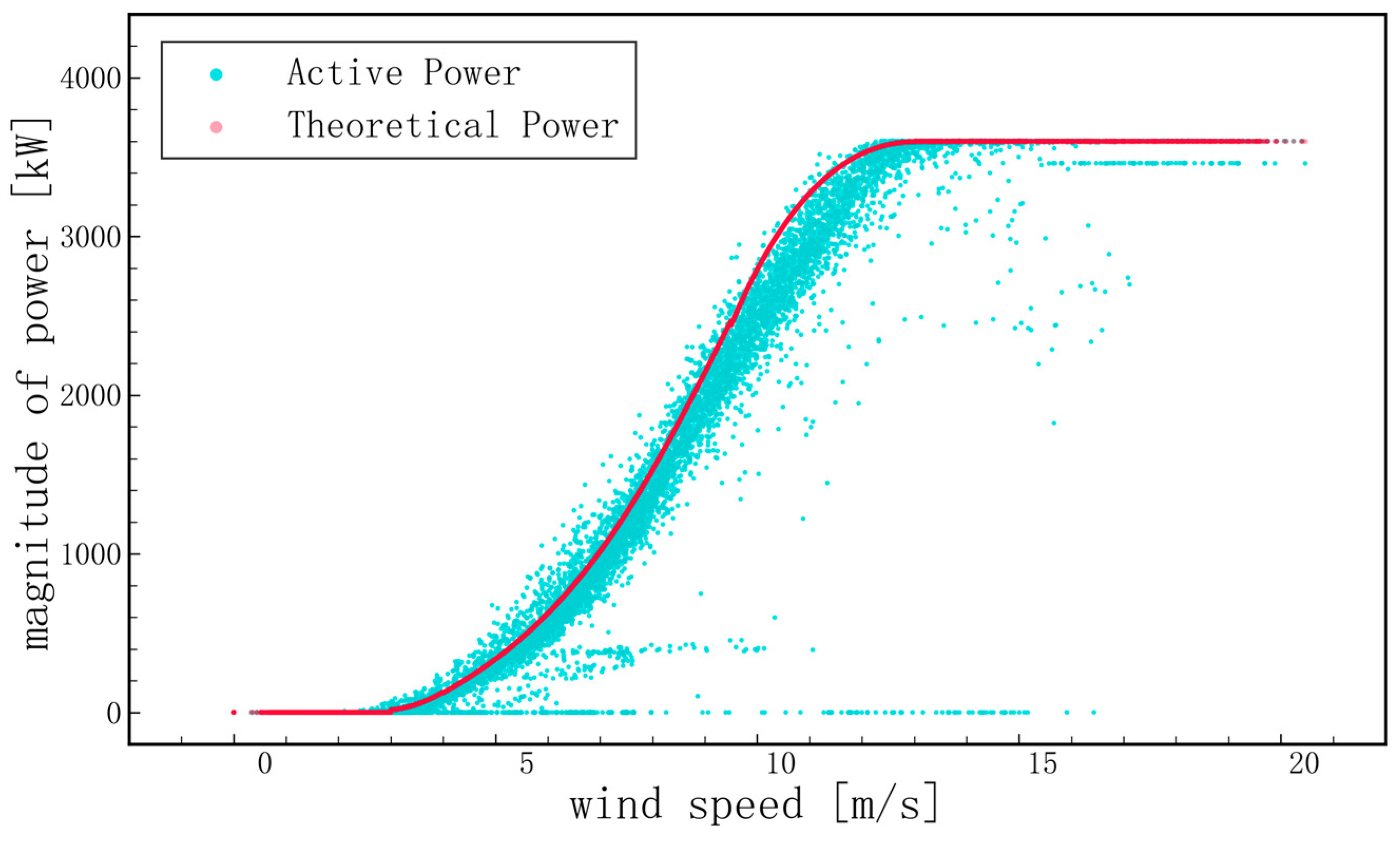
Under ideal operating conditions, the energy captured by the wind turbine can be modeled by Equation (13), which is the theoretical power value indicated in red in Figure 7. It can be seen that the theoretically available power is mainly positively related to the air density, the overflow area, and the wind speed cubic, in addition to the wind energy utilization factor described in Equations (14) and (15). The overflow area is fixed for the equipment, and the wind speed and direction records we collected are the main reference data for short-term predictions, since they contain seasonal variation characteristics and incoming flow characteristics in different directions, from which the machine-learning model can build a mapping to the power output at the next moment.
The wind energy that can be captured by wind turbines is as follows:
P w t b = 1 2 ρ C p ( λ , β ) π R 2 V w 3
The wind energy utilization coefficient is expressed as:
C p ( λ , β ) = 0.5 ( Γ 0.022 β 2 5.6 ) e 0.17 Γ
λ = ω w t b R V w ,   Γ = R λ 3600 1609
P w t b is the output power of the wind turbine (w); ρ is the air density ( k g / m 3 ) ; C p is the power coefficient; λ is the tip speed ratio; R is the blade radius (m); V w is the wind speed ( m / s ) ; ω w t b is the angular velocity of the wind turbine ( rad / s ) ; β is the blade pitch angle (°).
Figure 7 shows the scatter plot of the theoretical and actual power of the wind turbine corresponding to the wind speed. The red dots represent the theoretical power output of the wind turbine and the blue dots represent the actual power. According to the theoretical power calculation method for the wind turbine described before, wind speed is one of the most important direct influencing factors of power. The continuous motion of the atmospheric system is inertial, and the overall wind speed conditions around the turbine are easy to measure, so the power output can be predicted ahead of time in a short period of time based on continuous observation of the local wind speed.

3.1.3. Effect of Wind Direction

The default ideal case for calculating the power output of a wind turbine is to assume that the wind is coming in the direction of the impeller. However, even if the turbine can follow the wind direction in the actual state, the adjustment of the direction needs to overcome the inertia due to the huge size of the turbine equipment and takes some time to achieve. Therefore, the wind direction and turbine orientation are not always consistent, and only if the wind speed consistency is taken into account without considering the wind direction shift will the power prediction in advance lose accuracy.
Further, we can draw some inferences from Figure 8 that winds from another direction will also have different characteristics in terms of spatial velocity and turbulence. This has a non-negligible impact on the short-term power forecasts we are going to make, and wind changes should be used as important input information for the forecasts. It is also evident from Figure 9 that the distribution of significant wind speed intervals at all sample points is clearly correlated with the specific wind direction, and thus the concentrated distribution segments of the power output intervals also show consistency with it. In this study, the self-learning mechanism of neural networks is used for the time series prediction to explore the potential impact of wind speed and direction on the synergy of future short-term power output.

3.2. Evaluation Standard

Mean Absolute Error (MAE), Mean Absolute Error (MAE), Symmetric Mean Absolute Percentage Error (SMAPE), Mean Squared Error (MSE), Root Mean Squared Error (RMSE), and Coefficient of Determination ( R 2 ) are commonly used to evaluate the accuracy of forecasting methods: where y ^ i and y i are the predicted and actual values, and n is the total sample size.
M A E = 1 n i = 1 n y ^ i y i
S M A P E = 1 n i = 1 n y ^ i y i y ^ i + y i / 2 × 100 %
M S E = 1 n i = 1 n y ^ i y i 2
R M S E = 1 n i = 1 n y ^ i y i 2
R 2 = 1 i = 1 n y i y ^ i 2 i = 1 n y i y ¯ i 2

3.3. Pre-Processing of Signals

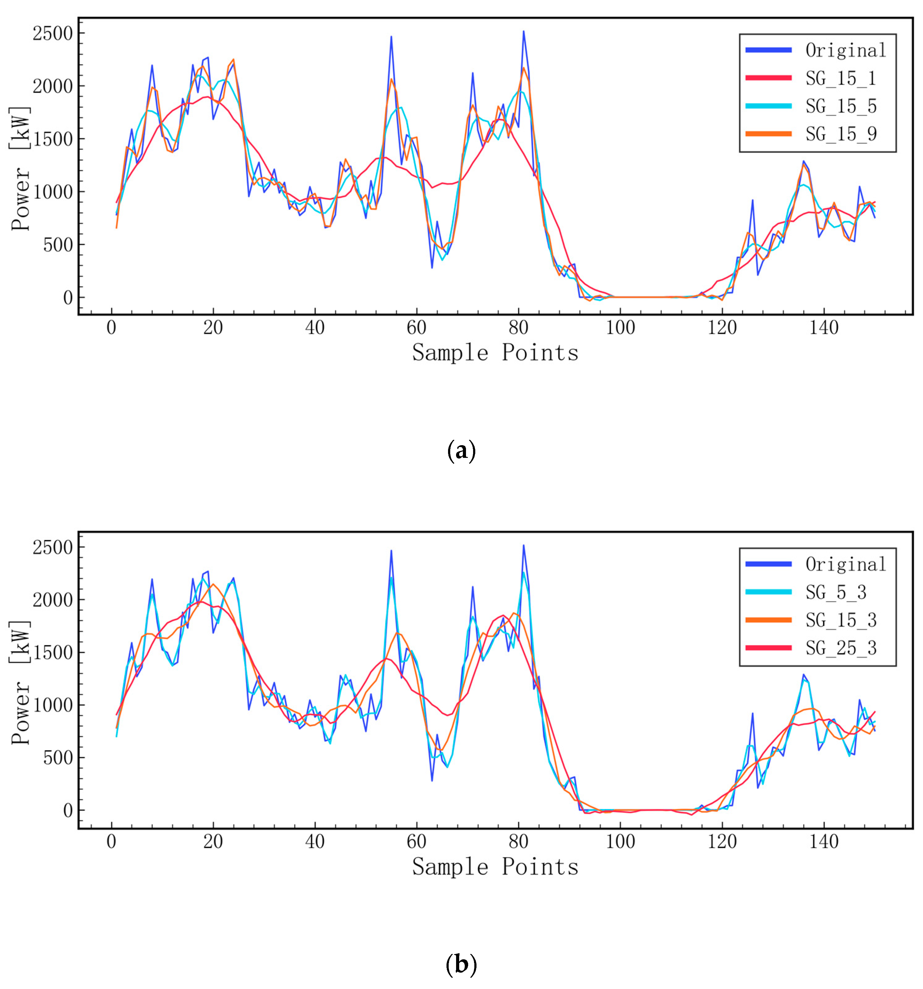
For the SG filter, there are two degrees of freedom that can be adjusted to suit the actual situation: the data frame length, and the polynomial order. From the filtering effect of the SG filter on the power signal demonstrated in Figure 10, it can be seen that the lower the polynomial order, the higher the degree of smoothing when the data frame length is the same (a); and the greater the data frame length, the higher the degree of smoothing when the polynomial order is the same (b).
The purpose of using filters is to degrade the noise, while the signal edge definition should be guaranteed, which is an advantage of the SG filter over the linear Moving Average (MA) filter [36]. To degrade the noise and ensure the signal edge definition, a lower polynomial order and a slightly larger data frame length are desirable. The literature [33] has set the frame length of the SG filter to 5, and the polynomial order to 2. Filters of order 2 but with progressively increasing frame length (3–31) were used for comparison in this study. The over-smoothed signal does not guarantee clear edges, which leads to poor performance of the trained model. The data frame length of 5 and the polynomial order of 2 are also valid in this case. The specific comparative test results are in Section 3.5.2.
Importantly, the input in the training phase was raw unfiltered data, and the output of the training set used filtered data, so the LSTM network that completed the training was able to overcome the noise of the actual signal and predict effectively.

3.4. Improved LSTM Network Model

In the prediction model, the LSTM neural network unit is selected as the component unit, and the weight of each input feature is updated through the backpropagation of the fully connected layer. The tensor calculation process of the predictor part is shown in Figure 11. The neural network node parameters are shown in Table 1. The implementation environment of the neural network model is Tensorflow2, on the Intel platform under the win10 system.
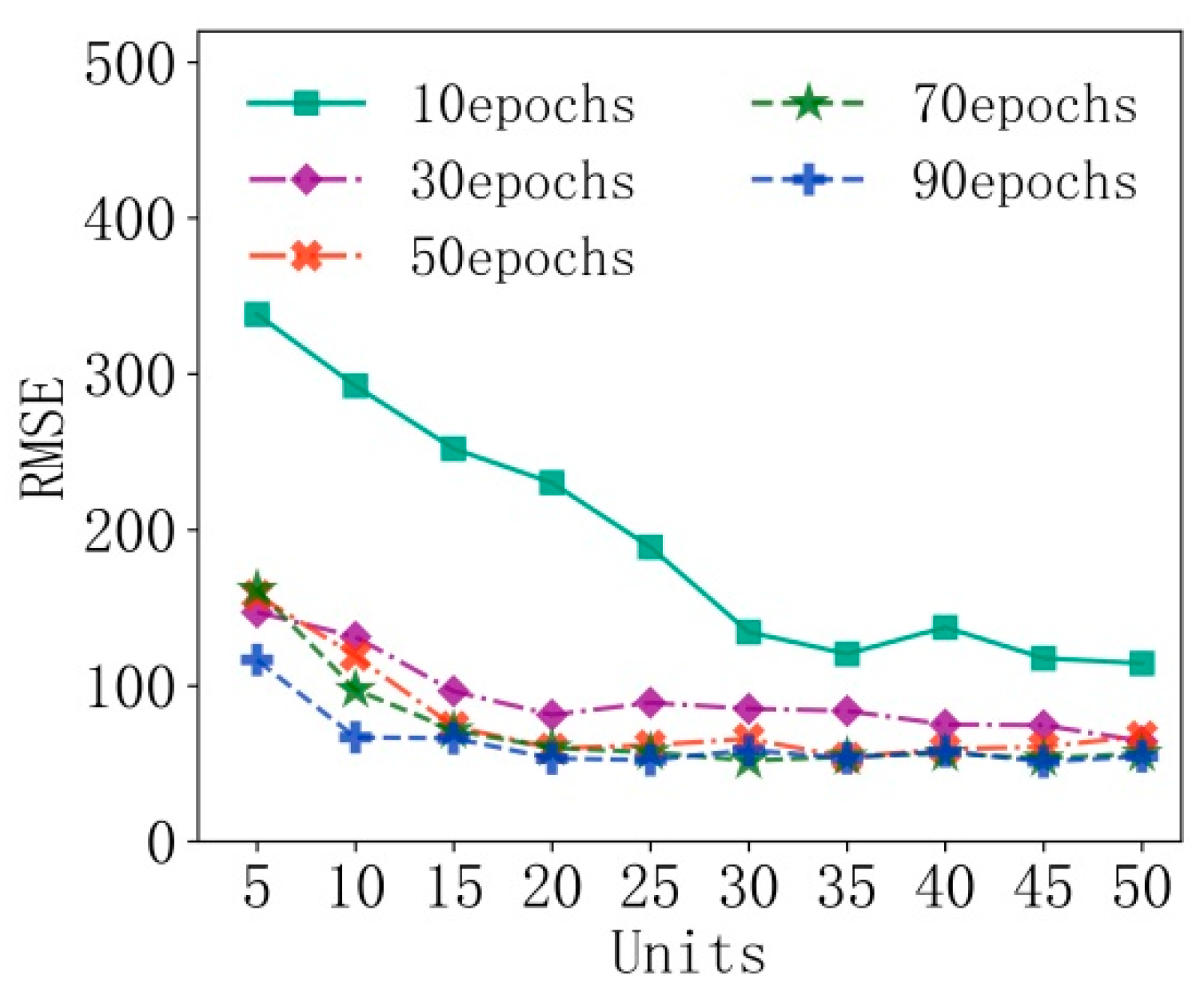
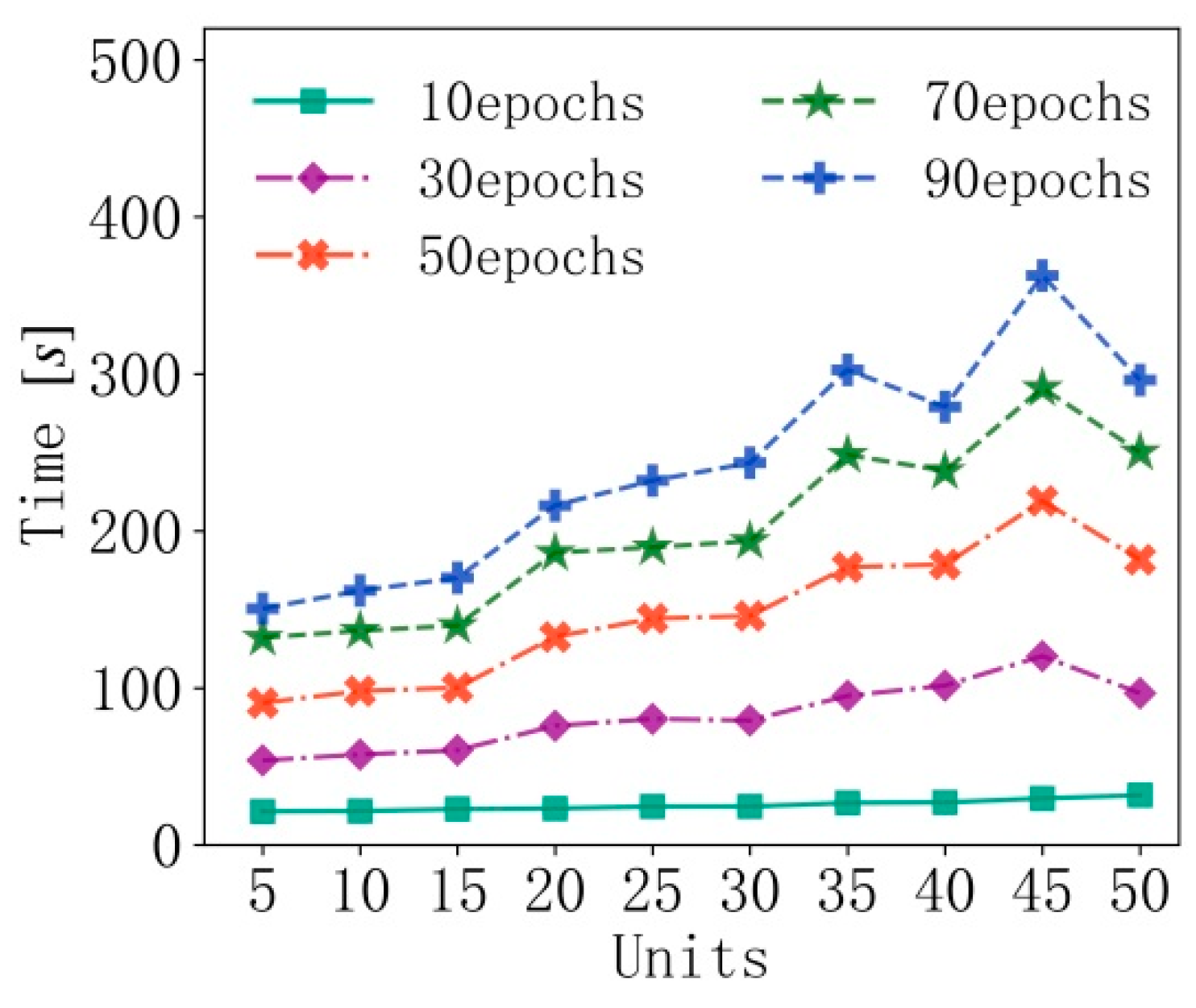
The LSTM neural network prediction model constructed in this study was set to three hidden stakes, and the influence of the number of computing units of and training times on the prediction results was explored. The number of computing units varies from five to 50, and the number of training times for model fitting varies from 10 to 100. As the complexity of the model increases and the number of fitting training increases, the accuracy of model prediction increases (Figure 12), but the computation time required also increases (Figure 13). The network model with the number of fittings increased to 100 and the number of computing units increased to 50 has tended to be consistent in terms of accuracy. The error fluctuation of the power prediction results under this condition was less than 0.5% of the rated power (3500 kW).

3.5. Presentation of Prediction Results and Analysis

3.5.1. Comprehensive Comparison of Models

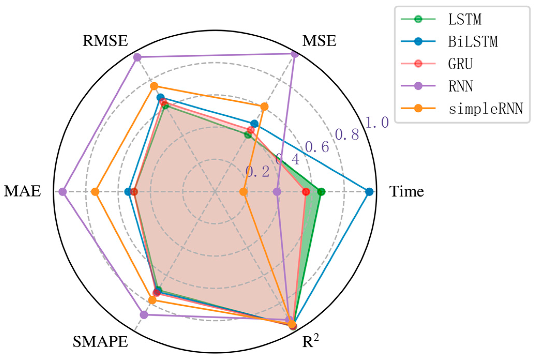
RNN, LSTM, GRU, and BiLSTM all adopted the structure of three hidden stakes, and simpleRNN was set to have only one hidden stake. All hidden stakes were set to have the same number of units, and the models were trained for 200 times with an input time step of 10. The evaluation indexes of the prediction results for several models are referred to in Figure 14 and Table 2.
The RNN series do not perform well in prediction. Although a neural network with multiple hidden stakes can theoretically fit any continuous function, the basic RNN model requires more training time and optimization improvements. The prediction errors of long short-term memory neural networks are all small and close to each other. Among them, BiLSTM is more time-consuming due to the two-way fitting calculation. Comprehensively comparing the accuracy and computational time of different methods, the long short-term memory neural network performs better in this time series information-mining task.

3.5.2. Single-Step Prediction

Machine-learning models perform time series prediction through a supervised learning framework. This training process requires using data from the training set as samples to learn from to obtain the patterns of variation in them. The output in the training set in this study is smoothed by a digital filter in pre-processing, which is equivalent to giving the machine-learning model a noise-filtering learning paradigm so that it can also output noise-reduced results in the prediction phase.
In order to determine the appropriate data frame length of the SG filter, filters of order 2 (N = 2) but with progressively increasing frame length (M = 1~15, frame length = 2M + 1 = 3~31) were used for comparison in this study (Table 3). A data frame length of 5 and a polynomial order of 2 are the most effective filtering parameters (MD2 in Table 3).
For the model that also used a second-order digital filter, the prediction error was not the same because the setting of the frame length changed the degree of smoothing. Values that are too small resulted in ineffective removal of noise (MD1), and values that are too large resulted in filtering out signal features other than noise (MD3–15). The presence of noise caused the model to learn these erroneous fluctuating features and fail to achieve accurate predictions when new data was input, i.e., poor generalization performance. However, the overuse of filters can lead to the loss of useful information, and the model trained in this case cannot effectively make predictions.
Among the series models with the filtering process added, MD2 has the smallest RMSE of 115.52. It has the best setting for the frame length. The RMSE of the LSTM without data processing is 247.4. The RMSE and the power value have the same magnitude, so for the whole power variation range (0–3500), the error reduction is 3.8%.
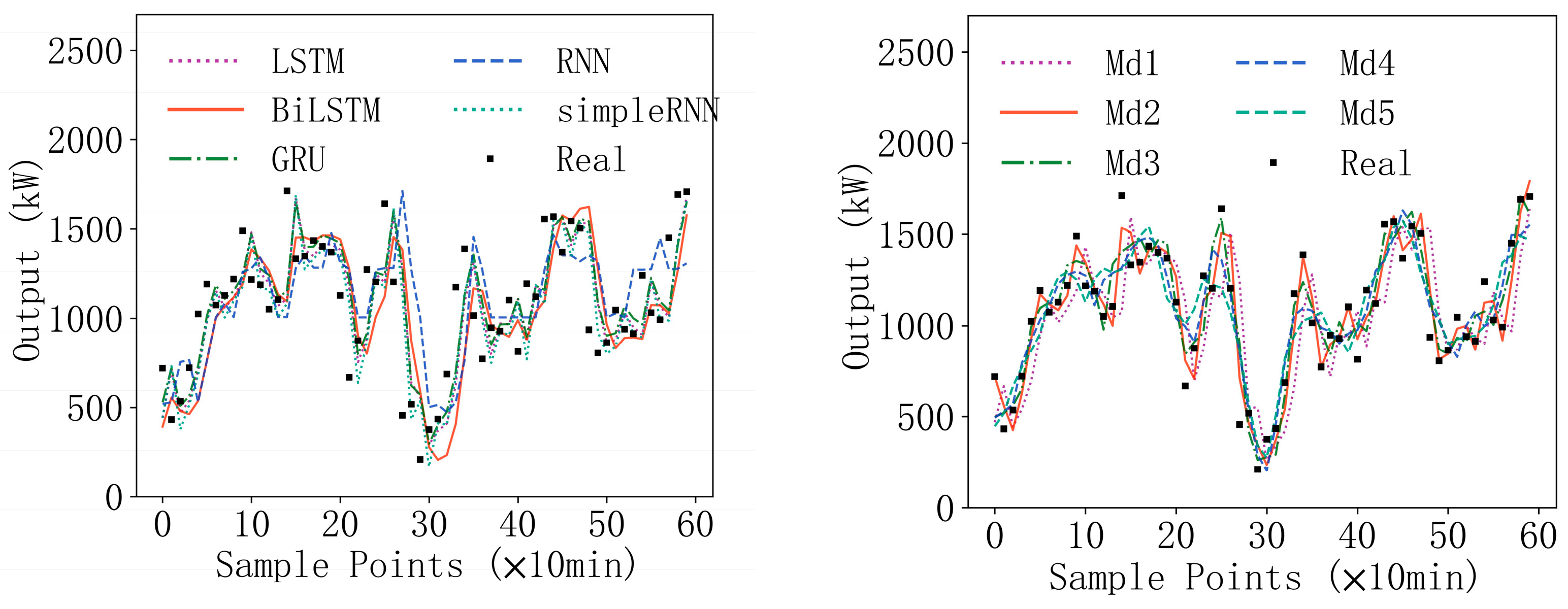
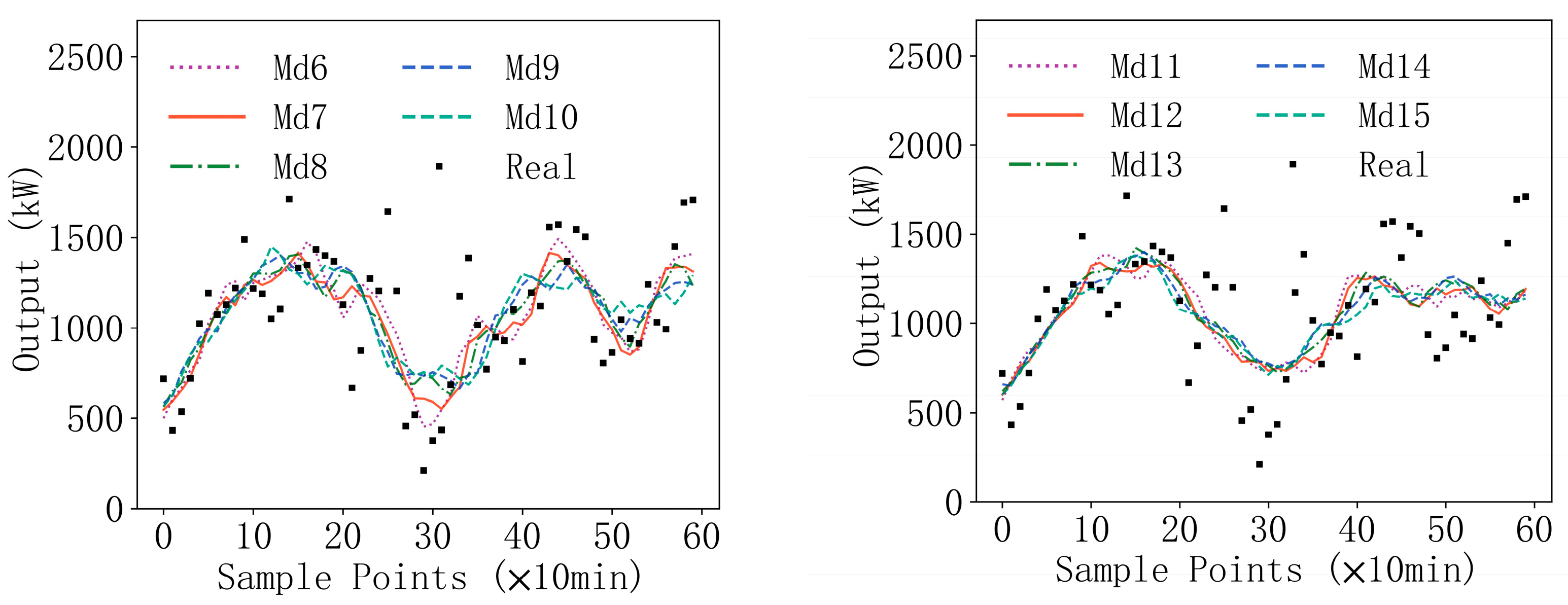
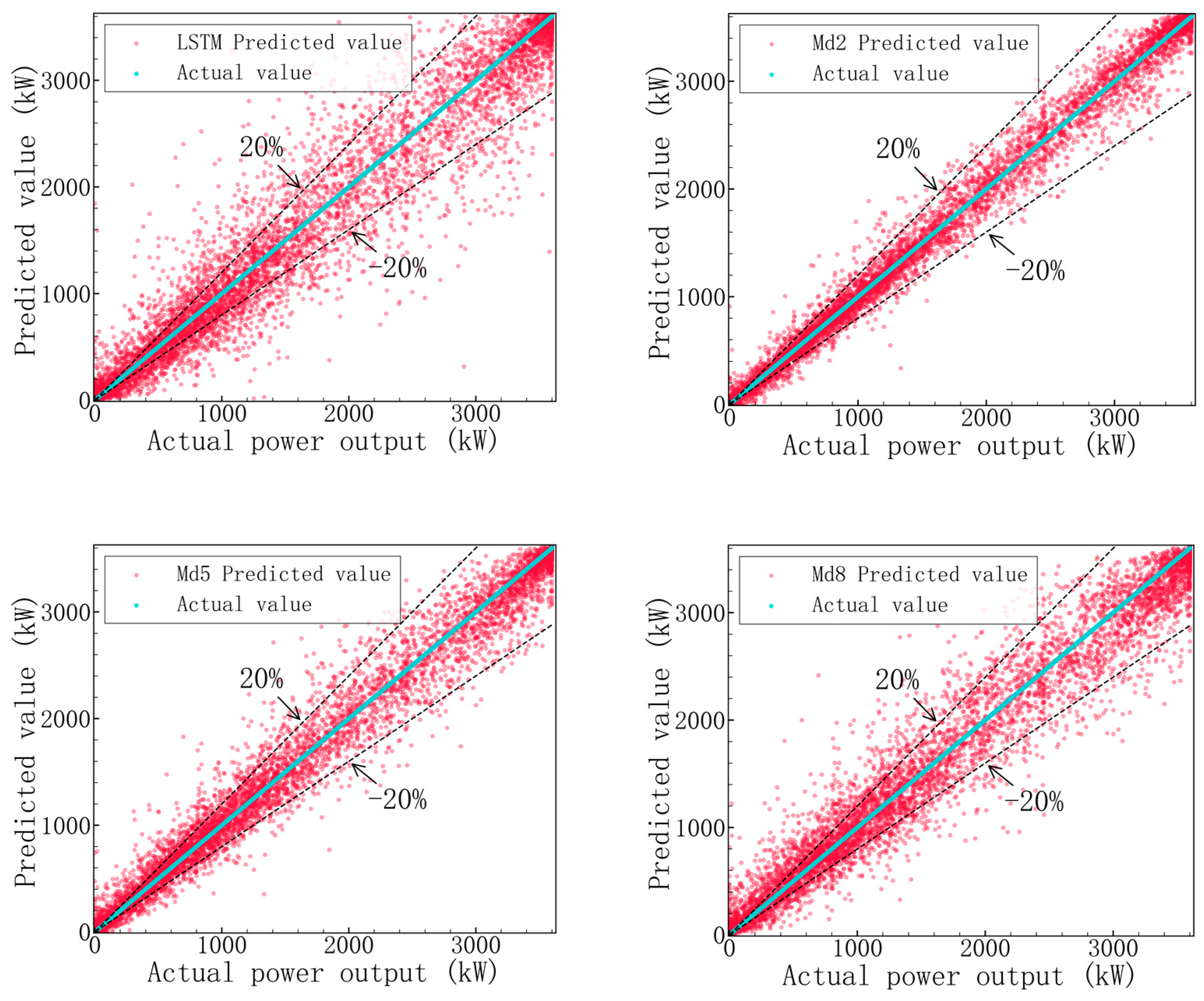
The predicted power curves from the different models are shown in Figure 15. The scatter of prediction results for the original model and several extracted optimization models are shown in Figure 16. The scattering of prediction results shows that the LSTM network model is able to overcome noise to achieve accurate and effective predictions by learning data pre-processed with the appropriate SG filter.

3.5.3. Multi-Step Prediction

Forecasting with multiple steps in advance gives the scheduling mechanism more time to schedule and execute the production plan. Different machine-learning models were used to implement multi-step forecasting with one to six steps, and the evaluation metrics are shown in Table 4. Figure 17 reflects the error variation law of the top ten multi-step prediction results. It can be seen that prediction errors generally tend to increase as the time step increases, so in order to obtain timely and valid prediction information, it is necessary to keep the error in each step as small as possible.
The LSTM controls the flow of information through a gating mechanism, thus avoiding the problem of vanishing or exploding gradients, and this allows the network to be more stable in dealing with long-term dependencies and produce better predictions when dealing with time-series data. In this study, the LSTM made full use of its strengths in this area by the time series modelling of meteorological parameters. Further data optimisation work was also implemented, with Savitzky-Golay filters optimising the expected output of the training set, and the most efficient configuration parameters were identified in the previous subsection. The improved data quality prevented the model from learning insignificant fluctuating features or noise, resulting in better generalisation performance. On the basis of these, the model achieved better results than other methods at all stages of the multi-step prediction. The normalized RMSEs for all six steps are 0.0485, 0.0772, 0.0932, 0.0109, 0.1168, and 0.1299, respectively, and the results of each step are the best among all the compared models. It can still maintain the prediction result at the fifth-step stage with a determination coefficient ( R 2 ) of 0.91. This accurate multi-step forecasting ensures the timeliness of effective forecasting information.

4. Summary and Conclusions

Achieving accurate wind power forecasting helps to specify scientific energy production plans in advance, which can help us to avoid supply and demand imbalance.
To enable the trained LSTM network model to overcome the effect of noise, the SG filter was used to process the output of the training set. Through test comparisons, it can be found that proper filtering parameters help to allow the model to learn data features better, thus showing better generalization performance in the test. The main findings are summarized as follows:
  • For the second-order SG filter, a data frame length setting of 5 is the best solution for signal quality improvement.
  • Optimization of the data used for learning allowed the RMSE of single-step prediction to decrease from 247.4 to 115.52, i.e., a 3.8% reduction in error over the range of values (0–3500 kW). The method is beneficial for improving the model’s generalization performance in testing.
  • From the multi-step prediction results, this method has the smallest prediction error at each step with normalized RMSEs of 0.0485, 0.0772, 0.0932, 0.0109, 0.1168, and 0.1299, respectively. The determination coefficient () remains 0.91 at the fifth step of prediction. The method is effective in increasing the timeliness of the prediction.
This study has not yet been combined with local weather forecasts to make more advanced forecasts of power output capacity. Therefore, numerical weather prediction can be further added to further improve the forecast timeliness.

Author Contributions

Investigation, S.L. and Y.Z.; resources, J.W.; data curation, S.L. and Y.Z.; writing—original draft preparation, S.L. and Y.Z.; visualization, T.X.; project administration, X.D.; funding acquisition, X.D. and J.W. All authors have read and agreed to the published version of the manuscript.

Funding

This research was funded by the Science and Technology Program for Youth of Gansu Province, grant number 21JR7RA262; the Science and Technology Program for Youth of Gansu Province, grant number 20JR10RA195; State Grid Integrated Energy Service Group Co.Ltd, grant number No.52789921001R; and 2022 Gansu Provincial University Industry Support Plan Project, grant number 2022CYZC-21.

Institutional Review Board Statement

Not applicable.

Informed Consent Statement

Not applicable.

Data Availability Statement

The data are available on request from the authors.

Conflicts of Interest

The authors declare no conflict of interest.

References

  1. BP. BP Statistical Review of World Energy; BP: London, UK, 2022. [Google Scholar]
  2. Qin, B.; Wang, M.; Zhang, G.; Zhang, Z. Impact of renewable energy penetration rate on power system frequency stability. Energy Rep. 2022, 8, 997–1003. [Google Scholar] [CrossRef]
  3. Dabar, O.A.; Awaleh, M.O.; Waberi, M.M.; Adan, A.-B.I. Wind resource assessment and techno-economic analysis of wind energy and green hydrogen production in the Republic of Djibouti. Energy Rep. 2022, 8, 8996–9016. [Google Scholar] [CrossRef]
  4. Saxena, A.; Shankar, R. Improved load frequency control considering dynamic demand regulated power system integrating renewable sources and hybrid energy storage system. Sustain. Energy Technol. Assess. 2022, 52, 102245. [Google Scholar] [CrossRef]
  5. Singh, B.; Sharma, A.K. Benefit maximization and optimal scheduling of renewable energy sources integrated system considering the impact of energy storage device and Plug-in Electric vehicle load demand. J. Energy Storage 2022, 54, 105245. [Google Scholar] [CrossRef]
  6. Niu, D.; Sun, L.; Yu, M.; Wang, K. Point and interval forecasting of ultra-short-term wind power based on a data-driven method and hybrid deep learning model. Energy 2022, 254, 124384. [Google Scholar] [CrossRef]
  7. Hu, W.C.; Yang, Q.S.; Zhang, P.; Yuan, Z.T.; Chen, H.P.; Shen, H.T.; Zhou, T.; Guo, K.P.; Li, T. A novel two-stage data-driven model for ultra-short-term wind speed prediction. Energy Rep. 2022, 8, 9467–9480. [Google Scholar] [CrossRef]
  8. Neshat, M.; Nezhad, M.M.; Abbasnejad, E.; Mirjalili, S.; Tjernberg, L.B.; Astiaso Garcia, D.; Alexander, B.; Wagner, M. A deep learning-based evolutionary model for short-term wind speed forecasting: A case study of the Lillgrund offshore wind farm. Energy Convers. Manag. 2021, 236, 114002. [Google Scholar] [CrossRef]
  9. Bett, P.E.; Thornton, H.E.; Troccoli, A.; De Felice, M.; Suckling, E.; Dubus, L.; Saint-Drenan, Y.-M.; Brayshaw, D.J. A simplified seasonal forecasting strategy, applied to wind and solar power in Europe. Clim. Serv. 2022, 27, 100318. [Google Scholar] [CrossRef]
  10. Ahmad, T.; Zhang, H.; Yan, B. A review on renewable energy and electricity requirement forecasting models for smart grid and buildings. Sustain. Cities Soc. 2020, 55, 102052. [Google Scholar] [CrossRef]
  11. Hwang, Y.-H.; Su, D.-T.; Yu, J.-L. A high resolution numerical method for solving atmospheric models. Chin. J. Phys. 2022, 77, 92–111. [Google Scholar] [CrossRef]
  12. Constantin, A.; Johnson, R.S. On the modelling of large-scale atmospheric flow. J. Differ. Equ. 2021, 285, 751–798. [Google Scholar] [CrossRef]
  13. Liu, X.; Lin, Z.; Feng, Z. Short-term offshore wind speed forecast by seasonal ARIMA—A comparison against GRU and LSTM. Energy 2021, 227, 120492. [Google Scholar] [CrossRef]
  14. Wang, Z.-X.; Li, Q.; Pei, L.-L. A seasonal GM(1,1) model for forecasting the electricity consumption of the primary economic sectors. Energy 2018, 154, 522–534. [Google Scholar] [CrossRef]
  15. Ding, S.; Hipel, K.W.; Dang, Y.-g. Forecasting China’s electricity consumption using a new grey prediction model. Energy 2018, 149, 314–328. [Google Scholar] [CrossRef]
  16. Suárez-Cetrulo, A.L.; Burnham-King, L.; Haughton, D.; Carbajo, R.S. Wind power forecasting using ensemble learning for day-ahead energy trading. Renew. Energy 2022, 191, 685–698. [Google Scholar] [CrossRef]
  17. Zhang, Y.; Li, Y.; Zhang, G. Short-term wind power forecasting approach based on Seq2Seq model using NWP data. Energy 2020, 213, 118371. [Google Scholar] [CrossRef]
  18. Blanchard, T.; Samanta, B. Wind speed forecasting using neural networks. Wind Eng. 2020, 44, 33–48. [Google Scholar] [CrossRef]
  19. Corizzo, R.; Ceci, M.; Fanaee-T, H.; Gama, J. Multi-aspect renewable energy forecasting. Inf. Sci. 2021, 546, 701–722. [Google Scholar] [CrossRef]
  20. Meka, R.; Alaeddini, A.; Bhaganagar, K. A robust deep learning framework for short-term wind power forecast of a full-scale wind farm using atmospheric variables. Energy 2021, 221, 119759. [Google Scholar] [CrossRef]
  21. Ding, S.; Tao, Z.; Li, R.; Qin, X. A novel seasonal adaptive grey model with the data-restacking technique for monthly renewable energy consumption forecasting. Expert Syst. Appl. 2022, 208, 118115. [Google Scholar] [CrossRef]
  22. Li, Z.; Luo, X.R.; Liu, M.J.; Cao, X.; Du, S.H.; Sun, H.X. Wind power prediction based on EEMD-Tent-SSA-LS-SVM. Energy Rep. 2022, 8, 3234–3243. [Google Scholar] [CrossRef]
  23. Yan, Y.; Wang, X.; Ren, F.; Shao, Z.; Tian, C. Wind speed prediction using a hybrid model of EEMD and LSTM considering seasonal features. Energy Rep. 2022, 8, 8965–8980. [Google Scholar] [CrossRef]
  24. Jaseena, K.U.; Kovoor, B.C. Decomposition-based hybrid wind speed forecasting model using deep bidirectional LSTM networks. Energy Convers. Manag. 2021, 234, 113944. [Google Scholar] [CrossRef]
  25. Liu, Y.; Guan, L.; Hou, C.; Han, H.; Liu, Z.; Sun, Y.; Zheng, M. Wind Power Short-Term Prediction Based on LSTM and Discrete Wavelet Transform. Appl. Sci. 2019, 9, 1108. [Google Scholar] [CrossRef] [Green Version]
  26. Liao, W.; Bak-Jensen, B.; Pillai, J.R.; Yang, Z.; Liu, K. Short-term power prediction for renewable energy using hybrid graph convolutional network and long short-term memory approach. Electr. Power Syst. Res. 2022, 211, 108614. [Google Scholar] [CrossRef]
  27. Dolatabadi, A.; Abdeltawab, H.; Mohamed, Y. Deep Spatial-Temporal 2-D CNN-BLSTM Model for Ultrashort-Term LiDAR-Assisted Wind Turbine’s Power and Fatigue Load Forecasting. IEEE Trans. Ind. Inform. 2022, 18, 2342–2353. [Google Scholar] [CrossRef]
  28. Li, L.-L.; Zhao, X.; Tseng, M.-L.; Tan, R.R. Short-term wind power forecasting based on support vector machine with improved dragonfly algorithm. J. Clean. Prod. 2020, 242, 118447. [Google Scholar] [CrossRef]
  29. Ewees, A.A.; Al-qaness, M.A.A.; Abualigah, L.; Abd Elaziz, M. HBO-LSTM: Optimized long short term memory with heap-based optimizer for wind power forecasting. Energy Convers. Manag. 2022, 268, 116022. [Google Scholar] [CrossRef]
  30. Neshat, M.; Nezhad, M.M.; Abbasnejad, E.; Mirjalili, S.; Groppi, D.; Heydari, A.; Tjernberg, L.B.; Garcia, D.A.; Alexander, B.; Shi, Q.F.; et al. Wind turbine power output prediction using a new hybrid neuro-evolutionary method. Energy 2021, 229, 120617. [Google Scholar] [CrossRef]
  31. Zhang, Z.; Ye, L.; Qin, H.; Liu, Y.; Wang, C.; Yu, X.; Yin, X.; Li, J. Wind speed prediction method using Shared Weight Long Short-Term Memory Network and Gaussian Process Regression. Appl. Energy 2019, 247, 270–284. [Google Scholar] [CrossRef]
  32. Xiong, B.R.; Lou, L.; Meng, X.Y.; Wang, X.; Ma, H.; Wang, Z.X. Short-term wind power forecasting based on Attention Mechanism and Deep Learning. Electr. Power Syst. Res. 2022, 206, 107776. [Google Scholar] [CrossRef]
  33. Zuo, B.; Cheng, J.; Zhang, Z. Degradation prediction model for proton exchange membrane fuel cells based on long short-term memory neural network and Savitzky-Golay filter. Int. J. Hydrog. Energy 2021, 46, 15928–15937. [Google Scholar] [CrossRef]
  34. Schafer, R.W. What Is a Savitzky-Golay Filter? [Lecture Notes]. IEEE Signal Process. Mag. 2011, 28, 111–117. [Google Scholar] [CrossRef]
  35. Lu, R.; Bai, R.; Huang, Y.; Li, Y.; Jiang, J.; Ding, Y. Data-driven real-time price-based demand response for industrial facilities energy management. Appl. Energy 2021, 283, 116291. [Google Scholar] [CrossRef]
  36. Angrisani, L.; Capriglione, D.; Cerro, G.; Ferrigno, L.; Miele, G. On Employing a Savitzky-Golay Filtering Stage to Improve Performance of Spectrum Sensing in CR Applications Concerning VDSA Approach. Metrol. Meas. Syst. 2016, 23, 295–308. [Google Scholar] [CrossRef]
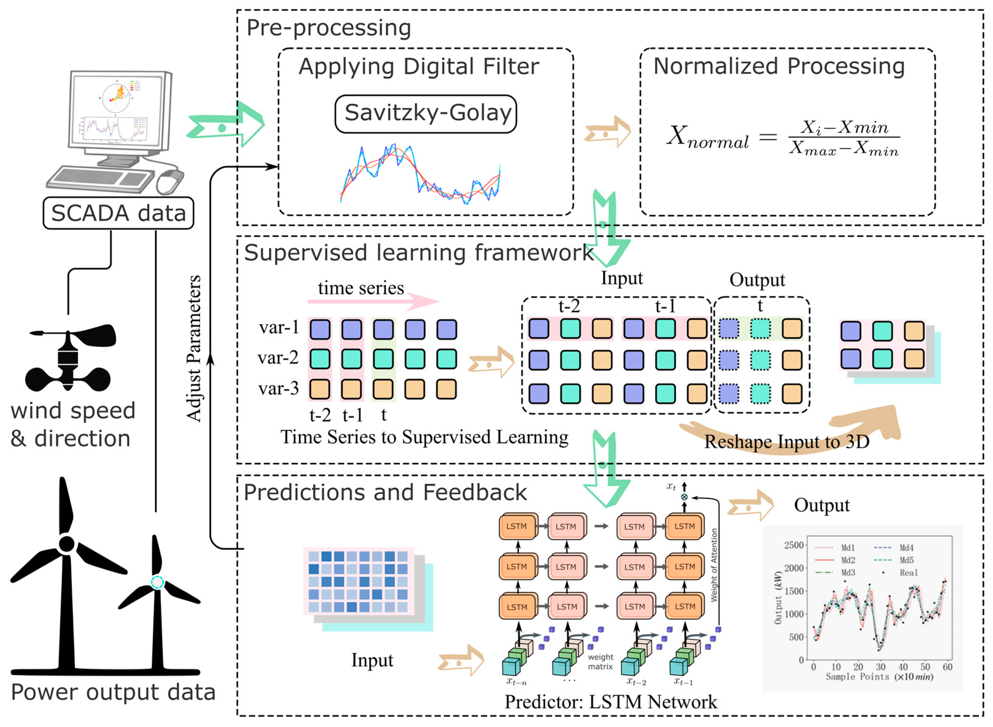
Figure 1. Data flow diagram of wind power short-term forecasting task framework.
Applsci 13 01751 g001
Figure 2. The time-unfolded computational graph of RNN.
Applsci 13 01751 g002
Figure 3. Schematic diagram of logical architecture of LSTM network unit.
Applsci 13 01751 g003
Figure 4. Schematic diagram of data processing flow of supervised learning task.
Applsci 13 01751 g004
Figure 5. Diagram of monthly distribution of wind speed.
Applsci 13 01751 g005
Figure 6. Power–wind speed curve.
Applsci 13 01751 g006
Figure 7. Power–wind speed distribution.
Applsci 13 01751 g007
Figure 8. Wind speed–orientation distribution map.
Applsci 13 01751 g008
Figure 9. Diagram of wind distribution and wind speed and power output corresponding to wind direction.
Applsci 13 01751 g009
Figure 10. Diagram of the effect of digital filtering. (a) The processing effect of filters with the same frame length but different orders. (b) The processing effect of filters with the same order but different frame lengths.
Applsci 13 01751 g010
Figure 11. Schematic diagram of multi-layer LSTM model.
Applsci 13 01751 g011
Figure 12. Schematic diagram of prediction error changing trend with epochs and units.
Applsci 13 01751 g012
Figure 13. Diagram of the variation trend of fitting time with epochs and units.
Applsci 13 01751 g013
Figure 14. Schematic diagram of comparison of prediction effect of basic model.
Applsci 13 01751 g014
Figure 15. Schematic diagram of power prediction results.
Applsci 13 01751 g015aApplsci 13 01751 g015b
Figure 16. Diagram of the scattering of predicted values.
Applsci 13 01751 g016
Figure 17. Error comparison chart of multi-step forecast.
Applsci 13 01751 g017
Table 1. Node parameter table of the neural network model.
Layer (Type)Output ShapeParam #Connected to
input_1 (InputLayer)(, 10, 3)0
lstm_1 (LSTM)(, 10, 64)17,408input_1[0][0]
dropout_1 (Dropout)(, 10, 64)0lstm_1[0][0]
lstm_2 (LSTM)(, 10, 3)816dropout_1[0][0]
dense_1 (Dense)(, 10, 3)12input_1[0][0]
dropout_2 (Dropout)(, 10, 3)0lstm_2[0][0]
attention_vec (Permute)(, 10, 3)0dense_1[0][0]
multiply_1 (Multiply)(, 10, 3)0dropout_2[0][0]
attention_vec[0][0]
flatten_1 (Flatten)(, 30)0multiply_1[0][0]
dense_2 (Dense)(, 1)31flatten_1[0][0]
Table 2. Performance comparison of basic neural network models.
ModelMSERMSEMAESMAPE/%R2Time/s
LSTM61,211.25247.40150.9256.340.965262
BiLSTM72,940.68270.07161.0357.310.957639
GRU66,200.80257.29150.8258.270.964503
RNN148,230.00385.00283.3070.560.913064
simpleRNN91,431.48302.37222.8162.090.941402
The better values for each indicator are marked in bold.
Table 3. Performance comparison between different models.
ModelRMSEMAESMAPE/%R2
LSTM247.40150.9256.340.96
BiLSTM270.07161.0357.310.95
GRU257.29150.8258.270.96
RNN385.00283.3070.560.91
simpleRNN302.37222.8162.090.94
Md1 (N = 2, M = 1)281.25169.7839.600.96
Md2 (N = 2, M = 2)115.5270.7632.270.99
Md3 (N = 2, M = 3)153.50104.5436.810.99
Md4 (N = 2, M = 4)170.99103.1134.700.98
Md5 (N = 2, M = 5)187.61116.9636.090.98
Md6 (N = 2, M = 6)202.78122.2738.390.98
Md7 (N = 2, M = 7)215.09130.5838.240.97
Md8 (N = 2, M = 8)226.97139.5437.130.97
Md9 (N = 2, M = 9)236.80144.9138.960.97
Md10 (N = 2, M = 10)248.04151.0240.060.97
Md11 (N = 2, M = 11)258.54160.9639.030.96
Md12 (N = 2, M = 12)266.47161.8840.730.96
Md13 (N = 2, M = 13)273.91169.6040.800.96
Md14 (N = 2, M = 14)282.26182.4640.310.95
Md15 (N = 2, M = 15)285.25175.5640.970.95
The better values in the accuracy indicators are marked in bold.
Table 4. Performance comparison of different models for forward multi-step power prediction.
MethodsError10 Min20 Min30 Min40 Min50 Min60 Min
Linear
Regression
nRMSE0.06140.08560.10140.11330.12360.1326
nMAE0.03580.05230.06320.07220.080.0868
R20.97270.94690.92550.90710.88940.8728
K-
Neighbors
nRMSE0.07890.10380.1220.13650.14980.1607
nMAE0.04690.06290.07460.08390.09280.1002
R20.95500.92200.89220.86520.83750.8131
RidgenRMSE0.06140.08560.10140.11330.12360.1325
nMAE0.03590.05230.06320.07220.08000.0868
R20.97270.94690.92550.90710.88940.8728
Random
Forest
nRMSE0.06670.09240.11030.12390.13360.1445
nMAE0.03950.05710.07000.07980.08720.0958
R20.96780.93820.91190.88880.87090.8489
xgBoostnRMSE0.06720.09460.11080.12450.13410.1457
nMAE0.03850.05570.06690.07650.08320.0914
R20.96730.93520.91110.88780.86990.8464
AdaboostnRMSE0.15450.18970.19630.20150.19770.1898
nMAE0.13200.15930.16380.17130.16480.1602
R20.82720.73960.72110.70620.71710.7393
SVRnRMSE0.07670.09810.11340.12450.1340.1426
nMAE0.06060.07540.08610.09340.09970.1057
R20.95740.93030.90690.88780.870.8528
MLPnRMSE0.06310.09050.10330.12250.12600.1350
nMAE0.03780.05860.06330.08390.07900.0886
R20.97120.94080.92280.89130.88500.8680
RNNnRMSE0.07190.10370.11780.11790.13060.1499
nMAE0.04660.07130.08430.07970.09010.1142
R20.96260.92220.89950.89940.87660.8373
LSTMnRMSE0.06360.08780.10310.11540.12670.1366
nMAE0.04130.05610.06330.07410.07990.0853
R20.97070.94420.92310.90370.88390.8650
Seq2SeqnRMSE0.15780.17060.12380.14260.15860.1608
nMAE0.12080.12880.08540.08940.11610.1226
R20.81980.78940.88910.85270.81790.8128
SG-LSTMnRMSE0.04850.07720.09320.10920.11680.1299
nMAE0.02970.04820.05780.07410.07510.0872
R20.98280.95630.93630.91260.90820.8763
The better values in each indicator are marked in bold.
Disclaimer/Publisher’s Note: The statements, opinions and data contained in all publications are solely those of the individual author(s) and contributor(s) and not of MDPI and/or the editor(s). MDPI and/or the editor(s) disclaim responsibility for any injury to people or property resulting from any ideas, methods, instructions or products referred to in the content.