Performance Analysis of Hybrid Kinematic Mechanism for Fusion Reactor Maintenance

Abstract

The hybrid kinematic mechanism (HKM) as an alternative remote handling subsystem of the Demonstration Fusion Power Plant (DEMO) breeding blanket (BB) is undergoing extensive theoretical analysis and feasibility verification. In this paper, the forward and inverse kinematic models of the HKM are derived by combining the Newtonian iterative method and the analytical method. Cartesian space trajectory planning is designed based on the trajectories of the HKM lifting of inboard and outboard BBs. The continuous smooth inverse kinematic solutions in the HKM joint space are obtained based on the polynomial interpolation method. For the characteristics of the HKM piston thread driving, the end-effector position error caused by the degradation of the spherical joint into a universal joint is analyzed and calculated. During the lifting of the left inboard BB, there is a maximum absolute error ∆P = 3.1 mm, and as the error continues to expand to the bottom of the BB it causes a risk of collision. Combining the overall effects of driving control, rigid–flexible coupling, etc., on position accuracy, an open-loop variable parameter error compensation plan based on the Levenberg–Marquardt (LM) nonlinear damping least-squares algorithm is proposed and validated in this paper. The simulation results show that the maximum absolute error after compensation is less than 1 mm as the mesh density increases, and the absolute position accuracy can be further improved by local mesh encryption. This study verifies the feasibility of the HKM as a BB remote handling subsystem and provides an option for high-precision control of the HKM.

1. Introduction

Under the European Fusion Development Agreement (EFDA), the EU is conducting a series of concept studies and development activities based on the Demonstration Fusion Power Plant (DEMO) [1]. Remote maintenance of the breeding blanket (BB) is a technical challenge that must be addressed before DEMO can operate commercially [2,3]. As shown in Figure 1, the Tokamak is currently designed to be maintained through 16–18 vertical ports from the top of the vacuum vessel, with each vertical port responsible for maintaining the corresponding five BBs [4,5]. The main functions of the BB are the following: (1) to achieve tritium multiplication and maintain the tritium needed for the fusion reactor; (2) to convert the energy produced by the fusion reactor into usable heat, electricity, etc.; (3) radiation shielding, to reduce the diffusion of reflective material and protect the magnet material. The gap between adjacent BBs in a vacuum vessel is only 20 mm, and with the largest BBs reaching a height of 10 m and a mass of about 80 tons, it is challenging to install and remove them precisely. The expected gamma radiation dosage during vacuum vessel maintenance is about 2000 Gy/h, which means that all operations must be remote, and the radiation level limits the selection of the technical solution.

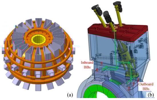
Figure 1. DEMO concept design (a); the process of HKM lifting the BBs (b).

The current design lifetime of BB in the DEMO vacuum vessel is 5 years. To determine the optimal maintenance design, DEMO conducted a large and extensive architectural research study, which concluded that Multi-Module Blanket Segments (MMS) and Vertical Maintenance Schemes (VMS) are the preferred layouts for maintenance [6,7]. For the design of the BB transporter, extensive brainstorming was conducted at an early stage, mainly on the comparison of the series kinematic mechanism (SKM), the parallel kinematic mechanism (PKM), and the hybrid kinematic mechanism (HKM) [8,9]. Through the preliminary evaluation of different structures and the feasibility analysis of the structures’ functions, an alternative BB maintenance scheme is proposed based on the HKM. As shown in Figure 1b, the configuration of the HKM is developed based on the classic Tricept parallel mechanism, which is a 3UPS-PU parallel mechanism with 3-DOFs. The end of the HKM is a series mechanism rotating around three axes, mounted on a Tricept parallel mechanism kinetic platform, which gives the HKM 6-DOFs the ability to meet the end-effector position and orientation control requirements. The maintenance task of the inboard and outboard BBs can be finished separately by the trajectory control of the HKM. The special advantage of the HKM is that it has relatively high stiffness, high load capacity, and high position accuracy [10], and at the same time has a relatively large working space and simple design of the series robot [11,12]. The HKM can achieve relatively large positioning and orientation capabilities; therefore, it is suitable for applications in confined spaces within vacuum vessels.

There are hundreds of existing PKMs, however, not many PKMs are used in the actual industrial production process. The main reason is that PKMs generally require a large number of passive joints in their design, and these passive joints will greatly increase the deformation and geometric errors of the whole machine under disturbance forces and overload conditions [13,14]. Therefore, many researchers have been exploring various hybrid mechanism design options. The development of the HKM based on the Tricept platform can achieve a large working space and positioning requirements, which have attracted a lot of attention [15]. This interest led to the development of the HKM and a large number of related papers. Li et al. [16,17] added 2-3-degree of freedom (DOF) wrists to the Tricept kinetic platform to form a 5-6-DOF hybrid robot and proposed an elastic dynamic modeling and dimensional synthesis method. Based on helical theory and structural dynamics, the kinetic and elastic potential energies of the Tricept mechanism and the series wrist were calculated [18]. Dong et al. [19] built the stiffness model of a novel five-DOF hybrid robot consisting of a Tricept parallel mechanism and a two-DOF wrist. Zheng et al. [20,21] proposed a hybrid mechanism consisting of two 3UPU mechanisms that can perform translational and yaw motions separately. Hu [22] investigated the complete kinematics of a hybrid robot composed of two (3SPS-UP) parallel robots connected in series. Hosseini et al. [23] optimized the workspace of the Tricept using a genetic algorithm.

In recent years, there has been an increasing number of studies on the accuracy analysis of parallel mechanisms considering geometric errors, joint errors, etc. [24]. Since the light link structure has unavoidable elastic deformation under large loads, which further causes large position errors, the position accuracy should be studied [25]. Ding et al. [26,27] simultaneously considered linkage elasticity, spherical joint, and universal joint clearance to evaluate the accuracy of Tricept under load, and the small changes in the link length caused by the clearance and deformation were simulated by a hyperbolic function. Yang et al. [28] proposed a nonlinear kinematic model for the flexible axis parallel mechanism. Wang et al. [29] identified geometric parameters according to the product of the exponentials (POE) formula and compensated for residual errors caused by non-geometric parameters using a multilayer perceptron neural network (MLPNN). Zhao et al. [30,31] proposed a modeling method for flexible parallel robots considering nonlinear friction characteristics, and used the least-squares method to complete parameter identification. Jiao et al. [32,33] proposed a sampling point selection method based on a spatial grid for static identification of kinematic parameters and joint stiffness. Liu et al. [34] established an error prediction model for the Tricept robot using a positional error decomposition strategy and a BP neural network (BPNN) to achieve high-precision real-time compensation. Wu et al. [35] proposed an iterative learning approach to compensate for the external uncertain dynamic loads of a 5-DOF hybrid-connected robot.

In this paper, based on the new HKM mechanism in a BB remote maintenance system, forward and inverse kinematic modeling is built. The trajectory planning of the HKM in Cartesian space and joint space is designed according to the remote maintenance process of the BBs. Due to the high self-weight of BBs and the fact that grease lubrication is not allowed in the vacuum vessel environment, the Tricept spherical joint in the HKM will degrade into a universal joint, causing position errors. Next, we focus on analyzing the possible errors after the degradation of the HKM and assessing the feasibility of engineering applications. To overcome the possible transmission error, control error, and rigid-flexible coupling deformation error, etc., an open-loop variable parameter error compensation algorithm is proposed to meet the actual needs of engineering.

This paper is organized as follows. Section 2 analyzes the forward and inverse kinematic properties of the HKM. Section 3 provides trajectory planning for the process of the HKM lifting BBs. Section 4 analyzes the effect of degradation of the Tricept spherical joint on the position accuracy of the HKM. Section 5 proposes an open-loop variable parameter error compensation method. Finally, Section 6 concludes this paper.

2. HKM Kinematic Analysis

The simplified geometry of the HKM studied in this paper is shown in Figure 2, which contains a parallel mechanism and a series mechanism. The parallel mechanism consists of the classic Tricept (3UPS-PU) mechanism, which contains a kinetic platform, three supporting pistons, a follower prismatic chain, and a static platform. Considering the constraints of the DEMO vacuum vessel, the three support pistons are arranged in an equilateral triangle configuration, and the structural design parameters are shown in Table 1. Since the vacuum vessel does not allow any oil contamination, a motor-threaded drive system is used to achieve motion control of each support piston of the parallel mechanism. By controlling the stroke of the three support pistons, the kinetic platform B₁, B₂, B₃ can be rotated along the x₁ and y₁ axes at the point P of the static platform. At the same time, they can be moved along the z₂ axis on the point O of the kinetic platform. Since the 3UPS-PU parallel mechanism has only three degrees of freedom, it cannot meet the requirement of the end-effector for any orientation adjustment in any position. Therefore, a series mechanism with three axes of rotation is fixed to the parallel mechanism kinetic platform to form the whole HKM, which can meet the requirement of orientation adjustment in any position.

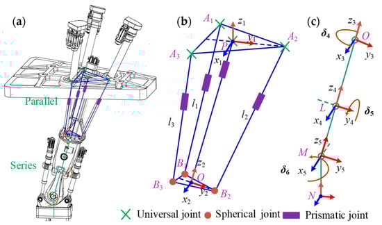
Figure 2. HKM structural features (a); HKM parallel mechanism coordinate system (b); HKM series mechanism coordinate system (c).

Table 1. The structure design parameters of the HKM.

No.	Variable	Value
1	lPAi	1000 mm
2	lA1B1	2510.68 mm
3	lA2B2	3032.78 mm
4	lA3B3	2814.66 mm
5	lOBi	475 mm
6	lOL	1800.00 mm
7	lLM	1250.00 mm
8	lMN	1025.00 mm
9	δ4	5.5°
10	δ5	8.56°
11	δ6	15.72°

2.1. HKM Forward Kinematics

The HKM parallel mechanism forward kinematics is solved by using both numerical and analytical methods. The analytical method mainly uses the elimination method to remove the unknown factors from the constraint equations of the mechanism and obtain a higher-order equation containing only the input and output parameters. This method can obtain all solutions of the mechanism, but the disadvantage is that the elimination process is very complicated, requires high computational accuracy, and is not universally applicable. Therefore, this paper uses the numerical method to solve the forward kinematics of the parallel mechanism. As shown in Figure 2, the nonlinear constraint equations for the parallel mechanism link length l_i are as follows:

$$\{\begin{array}{c}{f}_1\left(\alpha ,\beta ,z\right)=l_1^2-{\left(\stackrel{\rightharpoonup }{\mathit{P}\mathit{O}}+\stackrel{\rightharpoonup }{\mathit{O}{\mathit{B}}_{\mathbf{1}}}-\stackrel{\rightharpoonup }{\mathit{P}{\mathit{A}}_{\mathbf{1}}}\right)}^T\left(\stackrel{\rightharpoonup }{\mathit{P}\mathit{O}}+\stackrel{\rightharpoonup }{\mathit{O}{\mathit{B}}_{\mathbf{1}}}-\stackrel{\rightharpoonup }{\mathit{P}{\mathit{A}}_{\mathbf{1}}}\right)\\ f_2\left(\alpha ,\beta ,z\right)=l_2^2-{\left(\stackrel{\rightharpoonup }{\mathit{P}\mathit{O}}+\stackrel{\rightharpoonup }{\mathit{O}{\mathit{B}}_{\mathbf{2}}}-\stackrel{\rightharpoonup }{\mathit{P}{\mathit{A}}_{\mathbf{2}}}\right)}^T\left(\stackrel{\rightharpoonup }{\mathit{P}\mathit{O}}+\stackrel{\rightharpoonup }{\mathit{O}{\mathit{B}}_{\mathbf{2}}}-\stackrel{\rightharpoonup }{\mathit{P}{\mathit{A}}_{\mathbf{2}}}\right),\\ f_3\left(\alpha ,\beta ,z\right)=l_3^2-{\left(\stackrel{\rightharpoonup }{\mathit{P}\mathit{O}}+\stackrel{\rightharpoonup }{\mathit{O}{\mathit{B}}_{\mathbf{3}}}-\stackrel{\rightharpoonup }{\mathit{P}{\mathit{A}}_{\mathbf{3}}}\right)}^T\left(\stackrel{\rightharpoonup }{\mathit{P}\mathit{O}}+\stackrel{\rightharpoonup }{\mathit{O}{\mathit{B}}_{\mathbf{3}}}-\stackrel{\rightharpoonup }{\mathit{P}{\mathit{A}}_{\mathbf{3}}}\right)\end{array}$$

(1)

where α, β are the rotation angles of the kinetic platform around the x₁ axis and y₁ axis of point P, respectively, and z is the displacement of the follower prismatic chain.

The coordinates of the point O are the following:

$$\mathit{O}=\mathit{R}\mathit{o}\mathit{t}\left(y,\beta \right)\mathit{R}\mathit{o}\mathit{t}\left(x,\alpha \right)\mathit{T}\mathit{r}\mathit{a}\mathit{n}\mathit{s}\left(0, 0, \mathrm{z}\right),$$

(2)

where Rot is the rotation matrix and Trans is the translation matrix. Taking $\mathit{X}={\left[\begin{array}{ccc}\alpha & \beta & z\end{array}\right]}^T$, the following result is obtained after simplification.

$$f_i\left(\mathit{X}\right)=l_i^2-{\left(\mathit{P}\mathit{O}+\mathit{O}{\mathit{B}}_{\mathit{i}}-\mathit{P}{\mathit{A}}_{\mathit{i}}\right)}^T\left(\mathit{P}\mathit{O}+\mathit{O}{\mathit{B}}_{\mathit{i}}-\mathit{P}{\mathit{A}}_{\mathit{i}}\right).$$

(3)

Let the theoretical solution of this system of equations be ${\mathit{X}}^{*}={\left[\begin{array}{ccc}{\alpha }^{*}& {\beta }^{*}& z^{*}\end{array}\right]}^T$, then ${\mathit{X}}^{*}={\mathit{X}}_{\mathit{k}}+\mathit{\gamma }$, ${\mathit{X}}_{\mathit{k}}={\left[\begin{array}{ccc}{\alpha }_k& {\beta }_k& z_k\end{array}\right]}^T$ is the initial value of this nonlinear system of equations, and $\mathit{\gamma }={\left[\begin{array}{ccc}{\gamma }_1& {\gamma }_2& {\gamma }_3\end{array}\right]}^T$ is the error vector.

Expanding the Equation (3) at ${\mathit{X}}_{\mathit{k}}$ according to the Taylor series expansion, neglecting the higher-order partial derivatives and letting $f_i\left({\mathit{X}}_{\mathit{k}}+\mathit{\gamma }\right)$ converge to zero, we obtain

$$f_i\left({\mathit{X}}_{\mathit{k}}+\mathit{\gamma }\right)=f\left({\mathit{X}}_{\mathit{k}}\right)+\frac{\partial f_i}{\partial \alpha }{\gamma }_1+\frac{\partial f_i}{\partial \beta }{\gamma }_2+\frac{\partial f_i}{\partial z}{\gamma }_3.$$

(4)

When $f_i\left({\mathit{X}}_{\mathit{k}}+\mathit{\gamma }\right)=f\left({\mathit{X}}^{*}\right)=0$, a linear system of equations is obtained.

$$\left[\frac{\partial f_i}{\partial X_i}\right]\left[\mathit{\gamma }\right]=-\left[f\left({\mathit{X}}_{\mathit{i}}\right)\right].$$

(5)

Its expanded form is

$$\left[\begin{array}{ccc}\frac{\partial f_1}{\partial \alpha }& \frac{\partial f_1}{\partial \beta }& \frac{\partial f_1}{\partial z}\\ \frac{\partial f_2}{\partial \alpha }& \frac{\partial f_2}{\partial \beta }& \frac{\partial f_2}{\partial z}\\ \frac{\partial f_3}{\partial \alpha }& \frac{\partial f_3}{\partial \beta }& \frac{\partial f_3}{\partial z}\end{array}\right]\left[\begin{array}{c}{\gamma }_1\\ {\gamma }_2\\ {\gamma }_3\end{array}\right]=-\left[\begin{array}{c}{f}_1\\ f_2\\ f_3\end{array}\right].$$

(6)

The forward kinematics of this parallel mechanism can be solved by using the Newton–Raphson iterative method [36]. The constraint equations for the kinetic platform $\left[\alpha ,\beta ,z\right]$ with respect to the static platform and the rod length $l_i$ can be obtained as

$$\{\begin{array}{c}{f}_1\left(\alpha ,\beta ,z,l_1\right)=0\\ f_2\left(\alpha ,\beta ,z,l_2\right)=0\\ f_3\left(\alpha ,\beta ,z,l_3\right)=0\end{array}.$$

(7)

Solving the forward kinematics of the parallel mechanism is the process of finding the kinetic platform position $\left[\alpha ,\beta ,z\right]$ by giving the rod length $l_i$. Thus, when $l_i$ is taken as a known quantity, the system of equations can be abbreviated as

$$\mathit{f}\left(\mathit{x}\right)=0,$$

(8)

where $\mathit{x}={\left[\alpha ,\beta ,z\right]}^T$.

$$\mathit{f}\left(\mathit{x}\right)={\left[f_1\left(x\right),f_2\left(x\right),f_3\left(x\right)\right]}^T.$$

(9)

The iterative format for solving the nonlinear system of equations by Newton’s method is as follows:

$${\mathit{x}}_{\mathit{k}+\mathbf{1}}={\mathit{x}}_{\mathit{k}}+{\left[\mathit{J}\left({\mathit{x}}_{\mathit{k}}\right)\right]}^{-1}\mathit{f}\left({\mathit{x}}_{\mathit{k}}\right), k=0,1,2\cdots ,$$

(10)

$$\mathit{J}\left(\mathit{x}\right)=\left[\begin{array}{ccc}\frac{\partial f_1\left(x\right)}{\partial \alpha }& \frac{\partial f_1\left(x\right)}{\partial \beta }& \frac{\partial f_1\left(x\right)}{\partial z}\\ \frac{\partial f_2\left(x\right)}{\partial \alpha }& \frac{\partial f_2\left(x\right)}{\partial \beta }& \frac{\partial f_2\left(x\right)}{\partial z}\\ \frac{\partial f_3\left(x\right)}{\partial \alpha }& \frac{\partial f_3\left(x\right)}{\partial \beta }& \frac{\partial f_3\left(x\right)}{\partial z}\end{array}\right].$$

(11)

When the static platform of the parallel mechanism is locked in the position of the vertical ports of the vacuum vessel, the whole HKM can be equated to a 6-DOF series robot based on the forward kinematic solution $\left[\alpha ,\beta ,z\right]$. In order to represent the relationship between the motion of each joint, linkage and the end-effector, we use the Denavit–Hartenberg (DH) parameter method to establish the HKM forward kinematic model. The equivalent HKM kinematics equation established by DH parameters is as follows:

$${\mathit{T}}_{\mathbf{6}}^{\mathbf{0}}=\left[\begin{array}{cccc}{n}_x& o_x& a_x& p_x\\ n_y& o_y& a_y& p_y\\ n_z& o_z& a_z& p_z\\ 0& 0& 0& 1\end{array}\right]={\mathit{T}}_{\mathbf{1}}^{\mathbf{0}}\left(\beta \right){\mathit{T}}_{\mathbf{2}}^{\mathbf{1}}\left(\alpha \right){\mathit{T}}_{\mathbf{3}}^{\mathbf{2}}\left(z\right){\mathit{T}}_{\mathbf{4}}^{\mathbf{3}}\left({\delta }_4\right)\cdots {\mathit{T}}_{\mathbf{6}}^{\mathbf{5}}\left({\delta }_6\right),$$

(12)

where $\left[\mathit{n},\mathit{o},\mathit{a}\right]$ represents the end orientation of the HKM, $\left[p_x,p_y,p_z\right]$ represents the end position, and ${\mathit{T}}_{\mathit{i}}^{\mathit{i}-1}$ represents the coordinate transformation of adjacent joints. Based on the coordinate system in Figure 2, the DH parameters for the HKM equivalent to a series robot are shown in Table 2.

Table 2. HKM modified DH parameters.

Rod.i	Variable	Rotation Angle (°)	Distance (mm)
1	α	(14.83, 0, 0)	(0, 0, 0)
2	β	(0,10.04, 0)	(0, 0, 0)
3	z	(0,0,0)	(0, 0, 2740)
4	δ4	(0,0, 5.5)	(0, 0, 0)
5	δ5	(0, 8.56, 0)	(0, 0, −1800)
6	δ6	(15.72, 0, 0)	(0, 0, −1250)

2.2. HKM Inverse Kinematics

The inverse kinematics of the whole HKM are derived using following steps: First, the HKM geometry model is simplified. The HKM is a hybrid structure combining a parallel mechanism and a series mechanism. If both parallel and series mechanisms are considered in the inverse kinematic derivation, they will both determine the position and orientation of the end-effector. The position solution contains 3 independent equations, the orientation solution contains 9 non-independent equations, and 12 equations are solved for six unknowns, leading to a very complex solution process. To solve this problem, we simplify the parallel mechanism of HKM into a series mechanism, and equate the driving functions of the three pistons as the rotation around the x and y axes of the point $\mathit{P}\left(x_1,y_1,z_1\right)$ and the translational motion around the z axis of the point $\mathit{O}\left(x_2,y_2,z_2\right)$. The equivalent model is shown in Figure 3. The parallel mechanism is equated to a series mechanism, and its degrees of freedom are decomposed to a rotational motion around point P y₁ axis and x₂ axis, respectively, which constitute the universal joint. The prismatic motion of the kinetic platform is equated to the translational motion around the z₃ axis of point B. After simplification, the whole HKM can be regarded as a 6-DOF series robot.

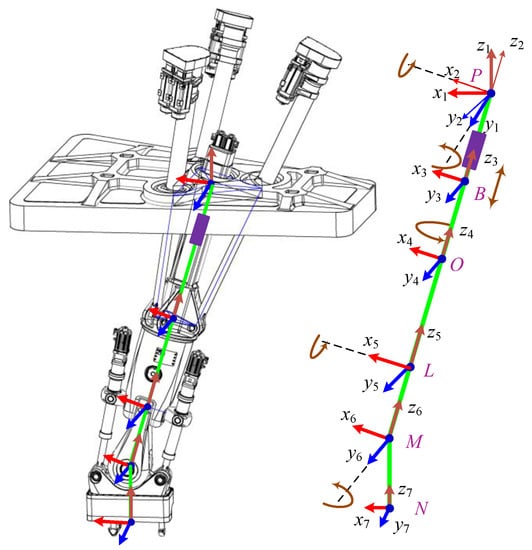
Figure 3. HKM simplified as a series mechanism.

Second, analytical and numerical methods were combined to calculate the HKM inverse kinematics. By analyzing the simplified HKM in Figure 3, we find that joints 1–4 share the same axis, so we can simplify the solution by reducing the number of unknowns in the system of equations by solving in the reverse direction from point N to point P. We assume that the position and orientation of the HKM endpoint N is:

$${\mathit{D}}_N=\left[\begin{array}{cccc}{n}_x& o_x& a_x& p_x\\ n_y& o_y& a_y& p_y\\ n_z& o_z& a_z& p_z\\ 0& 0& 0& 1\end{array}\right],$$

(13)

where $(n_i, o_i,a_i)$ denotes the end orientation and $\left(p_x, p_y,p_z\right)$ denotes the end position. The reverse direction kinematic equation of the HKM is established by the DH method:

$${\mathit{P}}_{\mathit{P}}={\mathit{D}}_{\mathit{N}}\ast {\mathit{D}}_{\mathbf{76}}\ast {\mathit{D}}_{\mathbf{65}}\ast {\mathit{P}}_{\mathbf{51}},$$

(14)

$${\mathit{D}}_{\mathbf{76}}=\left[\begin{array}{cccc}1& 0& 0& 0\\ 0& 1& 0& 0\\ 0& 0& 1& l_{MN}\\ 0& 0& 0& 1\end{array}\right]\ast \left[\begin{array}{cccc}c{\delta }_6& 0& s{\delta }_6& 0\\ 0& 1& 0& 0\\ -s{\delta }_6& 0& c{\delta }_6& 0\\ 0& 0& 0& 1\end{array}\right],$$

(15)

$${\mathit{D}}_{\mathbf{65}}=\left[\begin{array}{cccc}1& 0& 0& 0\\ 0& 1& 0& 0\\ 0& 0& 1& l_{LM}\\ 0& 0& 0& 1\end{array}\right]\ast \left[\begin{array}{cccc}1& 0& 0& 0\\ 0& c{\delta }_5& -s{\delta }_5& 0\\ 0& s{\delta }_5& c{\delta }_5& 0\\ 0& 0& 0& 1\end{array}\right],$$

(16)

$${\mathit{P}}_{\mathbf{51}}=\left[\begin{array}{c}0\\ 0\\ \begin{array}{c}{l}_{OL}+\mathrm{z}\\ 1\end{array}\end{array}\right],$$

(17)

where c denotes cos and s denotes sin. This convention will be adopted in future studies as well. Therefore, we simplify the HKM non-independent inverse kinematic equation system to an independent equation system containing only three unknowns $\mathit{\Phi }\left({\delta }_5,{\delta }_6,\mathrm{z}\right)$, as follows:

$$\{\begin{array}{c}{\mathit{\Phi }}_1=p_x+a_x{l}_{MN}+l_{LM}\left(a_{x}c{\delta }_6+n_{x}s{\delta }_6\right)-\left(l_{OL}+\mathrm{z}\right)\left(o_{x}s{\delta }_5-\mathrm{c}{\delta }_5\left(a_{x}c{\delta }_6+n_{x}s{\delta }_6\right)\right)\\ {\mathit{\Phi }}_2=p_y+a_y{l}_{MN}+l_{LM}\left(a_{y}c{\delta }_6+n_{y}s{\delta }_6\right)-\left(l_{OL}+\mathrm{z}\right)\left(o_{y}s{\delta }_5-\mathrm{c}{\delta }_5\left(a_{y}c{\delta }_6+n_{y}s{\delta }_6\right)\right).\\ {\mathit{\Phi }}_3=p_z+a_y{l}_{MN}+l_{LM}\left(a_{z}c{\delta }_6+n_{z}s{\delta }_6\right)-\left(l_{OL}+\mathrm{z}\right)\left(o_{z}s{\delta }_5-\mathrm{c}{\delta }_5\left(a_{z}c{\delta }_6+n_{z}s{\delta }_6\right)\right) \end{array}$$

(18)

The numerical and analytical methods can be used to solve the nonlinear equation system with three unknowns. Since we do not need the full analysis solution of the whole mechanism, we used the numerical method to solve the inverse kinematic solution of a simplified HKM. The numerical solution of Equation (18) was solved using the Newton–Raphson iterative method. The iterative format for solving the nonlinear system of equations by Newton’s method is shown as follows:

$$x_{k+1}=x_k+{\left[J\left(x_k\right)\right]}^{-1}f\left(x_k\right), k=0,1,2\cdots ,$$

(19)

$$\left[\mathit{J}\left(\mathit{x}\right)\right]=\left[\begin{array}{ccc}\frac{\partial f_1\left(x\right)}{\partial {\delta }_5}& \frac{\partial f_1\left(x\right)}{\partial {\delta }_6}& \frac{\partial f_1\left(x\right)}{\partial z}\\ \frac{\partial f_2\left(x\right)}{\partial {\delta }_5}& \frac{\partial f_2\left(x\right)}{\partial {\delta }_6}& \frac{\partial f_2\left(x\right)}{\partial z}\\ \frac{\partial f_3\left(x\right)}{\partial {\delta }_5}& \frac{\partial f_3\left(x\right)}{\partial {\delta }_6}& \frac{\partial f_3\left(x\right)}{\partial z}\end{array}\right].$$

(20)

By iterative calculation of Equation (19), we can obtain the partial solution of the HKM inverse kinematics $\left[{\delta }_5,{\delta }_6,z\right]$. The rest of the solutions $\left[\alpha ,\beta ,{\delta }_4\right]$ we calculated by the analytical method. Any point $\mathit{U}={\left[x_U,0,0,1\right]}^T.$ on the x₄ axis can be chosen within the coordinate system of point O in Figure 3. The kinematic equations of the point U are established from the points P and N, respectively, based on the DH method. From the equality of the coordinates of the point U in the forward (from point P) and reverse (from point N) kinematic equations, we can obtain:

$$\begin{array}{c}{\mathit{U}}_{\mathit{p}}={\mathit{D}}_{\mathbf{12}}\left(\beta \right){\mathit{D}}_{\mathbf{23}}\left(\alpha \right){\mathit{D}}_{\mathbf{34}}\left(z\right){\mathit{D}}_{\mathbf{54}}\left({\delta }_4\right) \mathit{U} \\ =\left[\begin{array}{c}{x}_U\left(c\beta c{\delta }_4+s\alpha s\beta s{\delta }_4\right)+zc\alpha s\beta \\ x_{U}c\alpha s{\delta }_4-\left(\mathrm{z}-l_{OL}\right)\mathrm{s}\alpha \\ \begin{array}{c}-x_U\left(s\beta c{\delta }_4-s\alpha c\beta s{\delta }_4\right)+zc\alpha c\beta \\ 1\end{array}\end{array}\right],\end{array}$$

(21)

$${\mathit{U}}_{\mathit{n}}={\mathit{D}}_N{\mathit{D}}_{\mathbf{76}}\left({\delta }_6\right){\mathit{D}}_{\mathbf{65}}\left({\delta }_5\right)\mathit{U}.$$

(22)

The parameters $\left[{\delta }_5,{\delta }_6,z\right]$ in the coordinate equation of the point $\mathit{U}$ are known. By letting $x_U=0$, the coordinates of the HKM forward kinematics ${\mathit{U}}_{\mathit{p}}$ and inverse kinematics ${\mathit{U}}_{\mathit{n}}$ at the point $\mathit{U}$ are equal, and we can obtain

$$\alpha =-arcs\left(\frac{{\mathit{U}}_{\mathit{n}}\left(2,1\right)}{z-l_{OL}}\right),$$

(23)

$$\beta =arcs\left(\frac{{\mathit{U}}_{\mathit{n}}\left(1,1\right)}{z\mathrm{c}\alpha }\right).$$

(24)

Letting $x_U\ne 0$, we can obtain

$${\delta }_4=arcs\left(\frac{{\mathit{U}}_{\mathit{n}}\left(2,1\right)+\left(\mathrm{z}-l_{OL}\right)\mathrm{s}\alpha }{x_U\mathrm{c}\alpha }\right).$$

(25)

Third, we calculated the HKM parallel mechanism inverse kinematic solution. Through the above calculations, we obtain the inverse kinematic solution $\left[\alpha ,\beta ,z,{\delta }_4,{\delta }_5,{\delta }_6\right]$ of the HKM equivalent to the series mechanism. The inverse kinematic solution of the HKM parallel mechanism is the process of solving for the stroke $\left(l_1,l_2,l_3\right)$ of each drive piston, by giving the position vector $\left(\alpha ,\beta ,z\right)$ of the end-effector. From Figure 3, we can obtain the position of point O under the coordinate system of point P as

$$\mathit{O}={\mathit{T}}_{\mathbf{1}}^{\mathbf{0}}\left(\beta \right){\mathit{T}}_{\mathbf{2}}^{\mathbf{1}}\left(\alpha \right){\mathit{T}}_{\mathbf{3}}^{\mathbf{2}}\left(z\right).$$

(26)

The stroke vector L_i and stroke length l_i of the piston in this parallel mechanism are

$${\mathit{L}}_{\mathit{i}}=\mathit{P}\mathit{O}+\mathit{O}{\mathit{B}}_{\mathit{i}}-\mathit{P}{\mathit{A}}_{\mathit{i}},$$

(27)

$$l_i=\sqrt{{\mathit{L}}_{\mathit{i}}{}^T{\mathit{L}}_{\mathit{i}}}=f_i\left(\beta ,\alpha ,z\right), i=1,2,3.$$

(28)

3. HKM Trajectory Planning

3.1. Cartesian Space Trajectory Planning

As shown in Figure 4 and Figure 5, to simplify the calculation, the trajectory of the HKM lifting BBs is represented by straight lines. There are five BBs, containing three outboard BBs and two inboard BBs. Here, the left outboard BB (marked in blue in Figure 4a) and left inboard BB (marked in blue in Figure 5a) are taken as examples to illustrate the whole process. Firstly, the center point between the three lifting twist locks of the HKM end-effector was set as the coordinate origin. Secondly the key dimensions and relative coordinate positions on the model were measured and calculated. Finally, the installation and disassembly of the BBs can be accomplished by successive inverse solutions of the HKM. See the online Supplementary Materials for a Video S1 of HKM lifting BBs.

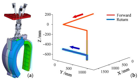
Figure 4. Left outboard BB position (a); lifting left outboard BB trajectory (b).

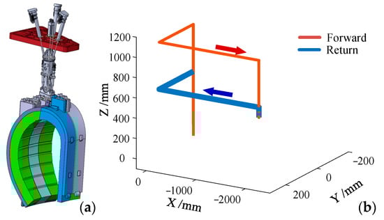
Figure 5. Left inboard BB position (a); lifting left inboard BB trajectory (b).

The motion trajectory is shown in Figure 4b and Figure 5b: the red trajectory shows the forward process of the HKM to engage and connect to the BBs, and the blue trajectory shows the return process of the HKM to remove the BBs.

3.2. Joint Space Trajectory Planning

With the designed Cartesian space trajectory planning, the discrete inverse kinematic solutions for each driving joint can be obtained. Here, the polynomial interpolation method for interpolation and fitting of discrete data are used. To simplify the computation and avoid excessive acceleration during velocity change, the cubic polynomial interpolation method was used to fit the discrete joint space inverse kinematic solutions.

The cubic polynomial interpolation method, as a commonly used interpolation method, has a continuous position and velocity curves and a variable acceleration, but the acceleration is not necessarily continuous. Consider the case of an interpolation between two data points, whose mathematical expression is the following:

$$q\left(t\right)=a_0+a_1\left(t-a_0\right)+a_2{\left(t-a_0\right)}^2+a_3{\left(t-a_0\right)}^3, t_0\le t\le t_1,$$

(29)

where $a_0, a_1, a_2, a_3$ are the coefficients to be determined.

Consider the case where two data points are given for interpolation if the position and velocity information $\left(q_0, q_1, v_0, v_1\right)$ at the initial moment $t_0$ and the final moment $t_1$ are given, and let $h=q_1-q_0, T=t_1-t_0$. Then, these parameters can be calculated using the following equations:

$$\{\begin{array}{c}{a}_0=q_0\\ a_1=v_0\\ \begin{array}{c}{a}_2=\frac{3h-\left(2v_0+v_1\right)T}{T^2}\\ a_3=\frac{-2h+\left(v_0+v_1\right)T}{T^3}\end{array}\end{array}.$$

(30)

For the case of interpolation given a series of n data points, the entire interpolation curve can be computed sequentially by using the above equation for both adjacent data points. Then, the continuous inverse kinematic solution of each driving joint of the HKM can be obtained as shown in Figure 6 and Figure 7.

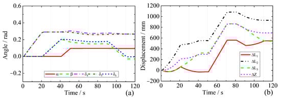
Figure 6. Lifting left outboard BB joint inverse kinematic solution (a); displacement inverse kinematic solution (b).

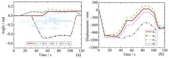
Figure 7. Lifting left inboard BB joint inverse kinematic solution (a); displacement inverse kinematic solution (b).

4. HKM Error Analysis

Since oil is not allowed in the high-temperature clean environment of the vacuum vessel, hydraulic drive and grease lubrication cannot be used. Therefore, each cylinder in the HKM parallel mechanism is driven by electrical power instead of a hydraulic system, as shown in Figure 8. The lubrication between each joint adopts dry friction lubrication. However, the weight of the BB is over 80 tons, thus, during the transportation of the BB, dry friction lubrication will cause a high torque on the spherical joint at one end of the piston, and it will be transferred to the cylinder in reverse. If the rotation between the piston rod and the cylinder is limited, the piston rod may suffer fatigue damage, so it must be allowed to rotate. From the abovementioned limitations, the HKM parallel mechanism spherical joints should be changed to universal joints during the BB lifting remote maintenance, where the rotation requirements of piston will be satisfied by the rotation between the piston and the cylinder, as shown in Figure 8b. The piston is driven by a ball screw, which will produce position error when the piston rotates relative to the cylinder.

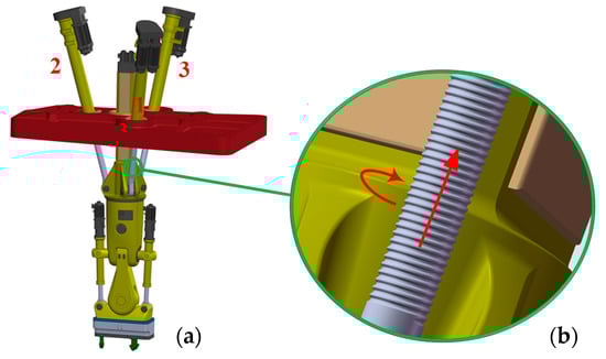
Figure 8. HKM prototype (a); piston thread drive mechanism (b).

In order to calculate the HKM end-effector position error caused by the piston rotation, an HKM simulation model was built in Adams software. Based on the inverse kinematic solution of the HKM lifting left inboard and outboard BBs obtained in Section 3, the piston rotation angle can be calculated by simulation in Adams, as shown in Figure 9. The results show that the piston rotates during the lifting of both the inboard and outboard BBs. During the lifting of the left outboard BB, piston 3 produces the maximum rotation angle $\Delta {\theta }_3=0.13 rad$ at the time of 40 s. During lifting of the left inboard BB, piston 3 produces the maximum rotation angle $\Delta {\theta }_3=0.19 rad$ at the time of 55 s. With the HKM of each piston’s thread at a pitch of $p=15 \mathrm{mm}$, combined with the angular error $\Delta {\theta }_i$, the stroke error of each piston can be obtained:

$$\Delta l_i=\frac{\Delta {\theta }_i}{2\pi }p.$$

(31)

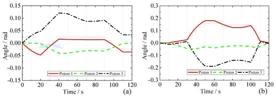
Figure 9. Rotation angle of HKM spherical joint around the link during the left outboard (a) and inboard (b) BB lifting.

By adding the obtained $\Delta l_i$ for each piston stroke error to the HKM inverse kinematic solution, the simulated position error of the HKM end-effector is obtained and is shown in Figure 10. The end-effector position error distribution is similar to the piston rotation angle error distribution. During the lifting of the left outboard BB, the end-effector produces a maximum absolute error $\Delta P=1.5 \mathrm{mm}$ at the moment of 40 s, and during the lifting of the left inboard BB, the end-effector produces a maximum absolute error $\Delta P=3.1 \mathrm{mm}$ at the moment of 55 s. Since the BB height is more than 10 m and the gap between adjacent BBs is only 20 mm, the large position error of the HKM on the $x$ and $y$ axes may hit the adjacent BBs to affect the stable motion of the HKM. In addition, the end position error is also influenced by the overall control error, rigid–flexible coupling deformation error, machining error, assembly error, creep error caused by wear, etc., which further causes the risk of collision. Therefore, it is necessary to compensate the end position error of the HKM to improve the operation accuracy.

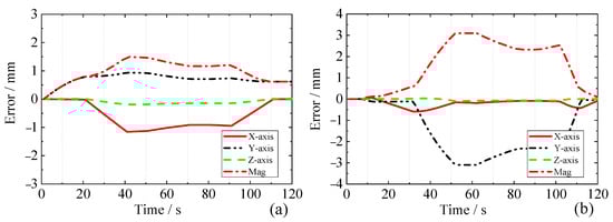
Figure 10. HKM end position error during the left outboard (a) and inboard (b) BB lifting.

5. Error Compensation

5.1. Variable Parameter Error Compensation

The HKM has a large working space, large load capacity and high position accuracy requirements. To avoid excessive stress on the HKM, the center of gravity of the load is always located directly below the HKM end twist locks during operation. Therefore, the requirements for the HKM dexterity are not high and the focus is on positional accuracy. In order to compensate for the global errors (including piston rotation error, control error, rigid–flexible coupling error, etc.) and to meet the requirements for fast adjustment of end position accuracy of the HKM, an open-loop variable parameter error compensation method is proposed, as shown in Figure 11. From the analysis of the HKM end position error in Section 4, the HKM end position error $\Delta \mathit{P}$ is obtained unevenly distributed in space. Therefore, it is not possible to compensate the error for the whole operating process by using a single parameter. Hence, the HKM workspace is meshed according to the error $\Delta \mathit{P}$ distribution. Under certain position accuracy requirements, each grid can adopt a set of parameters at the center point of the grid for error compensation. Different grids are solved separately for the compensation parameters to achieve variable parameter error compensation for the HKM workspace.

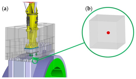
Figure 11. HKM workspace variable density meshing (a); a set of parameters is used to compensate for one grid region (b).

The flowchart of parameter error calculation within each grid is shown in Figure 12. First, we obtained the position error data of the HKM end-effector, and in order to simplify the calculation we take the end-effector position error caused by piston rotation as an example for variable parameter error compensation. Second, error modeling and preliminary meshing were performed. Since all kinds of errors such as piston rotation error, control error, and deformation error have certain influence on the end position accuracy of the HKM, and all of them are coupled with HKM kinematic parameters. Therefore, the errors of each parameter of the HKM can be expressed as a function of joint angle and piston stroke without considering the influence of random errors. The actual position Pr of the HKM end-effector can be expressed as

$${\mathit{P}}_r=\mathit{F}\left(\alpha +\Delta \alpha ,\beta +\Delta \beta ,\cdots ,{\delta }_6+\Delta {\delta }_6\right),$$

(32)

$$\begin{array}{c}\Delta \mathit{P}={\mathit{P}}_r-{\mathit{P}}_t \\ =\mathit{F}\left(\alpha +\Delta \alpha ,\beta +\Delta \beta ,\cdots ,{\delta }_6+\Delta {\delta }_6\right)-\mathit{F}\left(\alpha ,\beta ,\cdots ,{\delta }_6\right)\end{array},$$

(33)

where ${\mathit{P}}_t$ is the theory position of the HKM end-effector, $\Delta \mathit{P}$. is the position error, and the above equation can be linearized by discarding the higher order terms:

$$\Delta \mathit{P}=\frac{\partial \mathit{P}}{\partial \alpha }\Delta \alpha +\frac{\partial \mathit{P}}{\partial \beta }\Delta \beta +\cdots +\frac{\partial \mathit{P}}{\partial {\delta }_6}\Delta {\delta }_6.$$

(34)

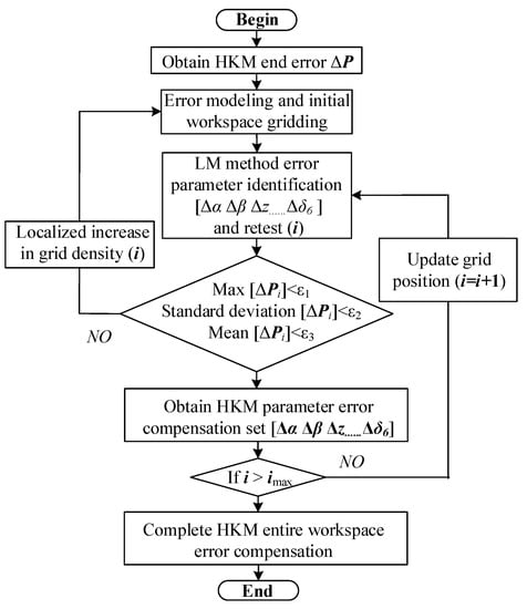
Figure 12. Flowchart of parameter error calculation within each grid.

By bringing in multiple sampling points for parameter identification of the parametric errors $\left[\Delta \alpha ,\Delta \beta ,\cdots ,\Delta {\delta }_6\right].$, the need for position error compensation within a single grid can be achieved.

Third, we performed the Levenberg–Marquardt method of parameter error identification [37]. For a single grid, a single parameter set can be used to compensate under the premise of satisfying a certain position accuracy. Parameter error calculation is a nonlinear parameter identification process.

$$\Delta \mathit{x}={\mathit{J}}^{-\mathbf{1}}\Delta \mathit{P},$$

(35)

where $\Delta \mathit{x}$ is the parametric error matrix and $\mathit{J}$ is the error Jacobian matrix. To solve for the parametric error $\Delta \mathit{x}$, we bring in the Levenberg–Marquardt (LM) nonlinear damped least-squares method for the identification of the parametric error. The LM algorithm is optimized with respect to the Gaussian–Newton method in terms of iteration steps, and the damping factor λ is introduced to avoid problems such as the singularity caused by the generalized inverse matrix. The iterative equation based on the LM algorithm is

$${\mathit{x}}^{k+1}={\mathit{x}}^k-{\left(\mathit{J}{\left({\mathit{x}}^k\right)}^{\mathit{T}}\mathit{J}\left({\mathit{x}}^k\right)+\mu \mathit{I}\right)}^{-1}\mathit{J}{\left({\mathit{x}}^k\right)}^{\mathit{T}}\Delta \mathit{P}\left({\mathit{x}}_k\right).$$

(36)

By iterative calculation, a set of compensation parameters $\left[\Delta \alpha ,\Delta \beta ,\cdots ,\Delta {\delta }_6\right]$ can be obtained, which are brought into the inverse kinematic solution of the HKM trajectory planning to complete the position error compensation.

Fourth, we judged the compensation effect. The maximum value, mean value, and standard deviation of the compensated residual error $\Delta {\mathit{P}}_i$ were calculated to judge whether the accuracy requirement is satisfied. If the accuracy requirement is not satisfied, the grid density was locally increased to identify the parameters again, and if the requirement is satisfied, it will continue to calculate the compensation parameters for the next grid. At the end of the cycle, the parameter error compensation values $\left[\Delta \mathit{\alpha },\Delta \mathit{\beta },\cdots ,\Delta {\mathit{\delta }}_{\mathbf{6}}\right]$ of the whole workspace can be obtained.

5.2. Analysis of Results

To verify the effect of variable parameter error compensation, we meshed the HKM working trajectory along with the time and performed parameter error identification and parameter error compensation, respectively. The compensation results are shown in Figure 13 and Figure 14. The specified estimate errors are shown in Table 3.

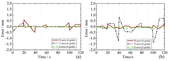
Figure 13. Lifting left outboard (a) and inboard (b) BB process end position error analysis.

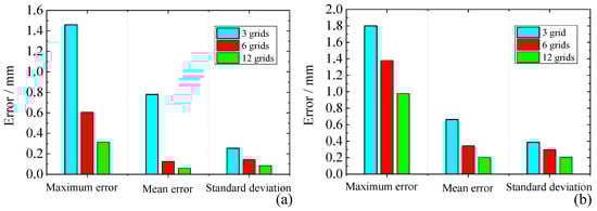
Figure 14. Lifting left outboard (a) and inboard (b) BB variable grid density results analysis.

Table 3. Estimate error of the HKM.

Grid Density	Maximum Error	Mean Error	Standard Deviation
3 grids	1.46 mm	0.78 mm	0.26 mm
6 grids	0.61 mm	0.13 mm	0.14 mm
12 grids	0.32 mm	0.06 mm	0.08 mm

Figure 13a,b show the residual position error of the end-effector during the HKM lifting the outboard and inboard BBs, respectively. After analyzing the results, we can obtain that the end position error is significantly reduced after compensation, but there are still large position errors at the moments of 20 s, 40 s, and 100 s. The main reason is that the grid density of these positions is small. When the HKM end-effector position error varies a large amount on a certain time series, using a set of parameters for error compensation will lead to poor compensation at the start and end moments. The use of local grid encryption can reduce the amount of position error variation within a single grid, which can effectively improve the compensation effect. Figure 14a,b and Table 3 show the compensation effect of the process of the HKM lifting the left outboard and inboard BBs with three grid densities. The results show that the maximum error, mean error, and standard deviation decrease significantly when the grid density increases. The higher the grid density, the higher the accuracy of the HKM end position, but with it, the computational amount also becomes larger. Reasonably limiting the accuracy index of the HKM end-effector and using a local grid encryption method will maximally solve the problems of accuracy and computational amount.

6. Conclusions

This paper first introduces an HKM for BB maintenance in a DEMO vacuum vessel, and then establishes the forward and inverse kinematic models of the HKM using a combination of analytical method and numerical iteration. By simulating the inboard and outboard BB remote maintenance process, the trajectory planning and simulation analysis of the HKM are carried out in Cartesian space and joint space, respectively, which validates the feasibility of the structure design. However, the high self-weight of 80 tons, the high working environment temperature, and the radiation environment in the vacuum vessel limited the selections of drive and lubrication systems for the HKM. The thread driving cylinder and dry friction lubrication degrade the spherical joint at one end of the piston into a universal joint, which causes position errors in the HKM end-effector. Through simulation, we calculated the error distribution caused by changing the spherical joint into a universal joint. During the lifting of the left outboard BB, the end-effector produces a maximum absolute error $\Delta P=1.5 \mathrm{mm}$, and during the lifting of the left inboard BB, the end-effector produces a maximum absolute error $\Delta P=3.1 \mathrm{mm}$. Combined with the overall effects of HKM rigid–flexible coupling deformation, assembly, machining, and other factors on the accuracy, the end position error will be further expanded. To compensate for the global errors, we propose a variable parameter error compensation plan based on the LM nonlinear damped least-squares algorithm. Error compensation can be realized through the HKM workspace gridding and offline parameter error identification. The simulation results show that the maximum error, mean error, and standard deviation at the end of the HKM are significantly reduced, which verifies the effectiveness of the compensation algorithm. The HKM has high stiffness, high load, and high precision compared to SKM, and a large working space compared to the PKM. It can achieve relatively large positioning and orientation capabilities and is suitable for applications in confined spaces within vacuum vessels.

In the future, we will further analyze the HKM end position accuracy by combining the dynamics and rigid–flexible coupling characteristics of the HKM. Then, various error factors will be incorporated into the HKM controller design to achieve HKM closed-loop control and online compensation of end position errors.

References

- Porton, M.; Latham, H.; Vizvary, Z.; Surrey, E. Balance of Plant Challenges for a Near-Term EU Demonstration Power Plant. In Proceedings of the 2013 IEEE 25th Symposium on Fusion Engineering (SOFE), San Francisco, CA, USA, 10–14 June 2013; pp. 1–6. [Google Scholar]
- Crofts, O.; Harman, J. Maintenance duration estimate for a DEMO fusion power plant, based on the EFDA WP12 pre-conceptual studies. Fusion Eng. Des. 2014, 89, 2383–2387. [Google Scholar] [CrossRef]
- Budden, S. Concept Design Description for MMS Blanket Transporter PoP Concept Design; EURO Fusion: Garching, Germany, 2019; EFDA_D_2MRZLG v2.2.; Available online: https://idm.euro-fusion.org/?uid=2MRZLG (accessed on 3 December 2022).
- Coleman, M.; Sykes, N.; Cooper, D.; Iglesias, D.; Bastow, R.; Loving, A.; Harman, J. Concept for a vertical maintenance remote handling system for multi-module blanket segments in DEMO. Fusion Eng. Des. 2014, 89, 2347–2351. [Google Scholar] [CrossRef]
- Fernández-Berceruelo, I.; Palermo, I.; Urgorri, F.R.; Rapisarda, D.; Garcinuño, B.; Ibarra, Á. Remarks on the performance of the EU DCLL breeding blanket adapted to DEMO 2017. Fusion Eng. Des. 2020, 155, 111559. [Google Scholar] [CrossRef]
- Loving, A.; Crofts, O.; Sykes, N.; Iglesias, D.; Coleman, M.; Thomas, J.; Harman, J.; Fischer, U.; Sanz, J.; Siuko, M.; et al. Pre-conceptual design assessment of DEMO remote maintenance. Fusion Eng. Des. 2014, 89, 2246–2250. [Google Scholar] [CrossRef]
- Iglesias, D.; Bastow, R.; Cooper, D.; Crowe, R.; Middleton-Gear, D.; Sibois, R.; Carloni, D.; Vizvary, Z.; Crofts, O.; Harman, J.; et al. Remote handling assessment of attachment concepts for DEMO blanket segments. Fusion Eng. Des. 2015, 98–99, 1500–1504. [Google Scholar] [CrossRef]
- Yen, P.-L.; Wang, C.-H.; Lin, H.-T.; Hung, S.-S. Optimization design for a compact redundant hybrid parallel kinematic machine. Robot. Comput.-Integr. Manuf. 2019, 58, 172–180. [Google Scholar] [CrossRef]
- Xu, P.; Cheung, C.F.; Li, B.; Wang, C.; Zhao, C. Design, Dynamic Analysis, and Experimental Evaluation of a Hybrid Parallel–Serial Polishing Machine With Decoupled Motions. J. Mech. Robot. 2021, 13, 061008. [Google Scholar] [CrossRef]
- Yun, Y.A.; Li, Y. Design and analysis of a novel 6-DOF redundant actuated parallel robot with compliant hinges for high precision positioning. Nonlinear Dynam. 2010, 61, 829–845. [Google Scholar] [CrossRef]
- Uriarte, L.; Zatarain, M.; Axinte, D.; Yagüe-Fabra, J.; Ihlenfeldt, S.; Eguia, J.; Olarra, A. Machine tools for large parts. CIRP Ann. 2013, 62, 731–750. [Google Scholar] [CrossRef]
- Bi, Z.M.; Jin, Y. Kinematic modeling of Exechon parallel kinematic machine. Robot. Comput.-Integr. Manuf. 2011, 27, 186–193. [Google Scholar] [CrossRef]
- Luces, M.; Mills, J.K.; Benhabib, B. A Review of Redundant Parallel Kinematic Mechanisms. J. Intell. Robot. Syst. 2017, 86, 175–198. [Google Scholar] [CrossRef]
- Neumann, K.E. Adaptive in-jig high load Exechon machining & assembly technology. In Proceedings of the 2018 Aerospace Manufacturing and Automated Fastening Conference & Exhibition, North Charleston, SC, USA, 16–18 September 2008; pp. 1–7. [Google Scholar]
- Huang, T.; Dong, C.; Liu, H.; Sun, T.; Chetwynd, D.G. A simple and visually orientated approach for type synthesis of overconstrained 1T2R parallel mechanisms. Robotica 2018, 37, 1161–1173. [Google Scholar] [CrossRef]
- Dong, C.; Liu, H.; Huang, T.; Chetwynd, D.G. A Screw Theory-Based Semi-Analytical Approach for Elastodynamics of the Tricept. Robot. J. Mech. Robot. 2019, 11, 031005. [Google Scholar] [CrossRef]
- Li, J.; Ye, F.; Shen, N.; Wang, Z.; Geng, L. Dimensional synthesis of a 5-DOF hybrid robot. Mech. Mach. Theory. 2020, 150, 103865. [Google Scholar] [CrossRef]
- Xu, Q.S.; Li, Y.M. An investigation on mobility and stiffness of a 3-DOF translational parallel manipulator via screw theory. Robot. Comput.-Integr. Manuf. 2008, 24, 402–414. [Google Scholar] [CrossRef]
- Dong, C.; Liu, H.; Yue, W.; Huang, T. Stiffness modeling and analysis of a novel 5-DOF hybrid robot. Mech. Mach. Theory. 2018, 125, 80–93. [Google Scholar] [CrossRef]
- Zheng, X.Z.; Bin, H.Z.; Luo, Y.G. Kinematic analysis of a hybrid serial-parallel manipulator. Int. J. Adv. Manuf. Technol. 2004, 23, 925–930. [Google Scholar] [CrossRef]
- Gallardo-Alvarado, J.; Posadas-García, J.D. Mobility analysis and kinematics of the semi-general 2(3-RPS) series-parallel manipulator. Robot. Comput.-Integr. Manuf. 2013, 29, 463–472. [Google Scholar] [CrossRef]
- Hu, B. Complete kinematics of a serial–parallel manipulator formed by two Tricept parallel manipulators connected in serials. Nonlinear. Dynam. 2014, 78, 2685–2698. [Google Scholar] [CrossRef]
- Hosseini, M.A.; Daniali, H.M. Cartesian workspace optimization of Tricept parallel manipulator with machining application. Robotica 2014, 33, 1948–1957. [Google Scholar] [CrossRef]
- Wu, J.; Wang, J.; You, Z. An overview of dynamic parameter identification of robots. Robot. Comput.-Integr. Manuf. 2010, 26, 414–419. [Google Scholar] [CrossRef]
- Tang, T.; Zhang, J. Conceptual design and kinetostatic analysis of a modular parallel kinematic machine-based hybrid machine tool for large aeronautic components. Robot. Comput.-Integr. Manuf. 2019, 57, 1–16. [Google Scholar] [CrossRef]
- Ding, J.Z.; Wang, C.J. Accuracy analysis and error compensation for Tricept machine tool under load. J. Mech. Sci. Technol. 2021, 35, 3591–3600. [Google Scholar] [CrossRef]
- Aginaga, J.; Altuzarra, O.; Macho, E.; Iriarte, X. Assessing Position Error Due to Clearances and Deformations of Links in Parallel Manipulators. J. Mech. Design. 2013, 135, 041006. [Google Scholar] [CrossRef]
- Yang, M.; Du, Z.; Chen, F.; Dong, W.; Zhang, D. Kinetostatic modelling of a 3-PRR planar compliant parallel manipulator with flexure pivots. Precis. Eng. 2017, 48, 323–330. [Google Scholar] [CrossRef]
- Wang, Y.; Chen, Z.; Zu, H.; Zhang, X.; Mao, C.; Wang, Z. Improvement of Heavy Load Robot Positioning Accuracy by Combining a Model-Based Identification for Geometric Parameters and an Optimized Neural Network for the Compensation of Nongeometric Errors. Complexity 2020, 30, 5896813. [Google Scholar] [CrossRef]
- Zhao, L.; Zhao, X.-H.; Li, B.; Yang, Y.-W.; Liu, L. Nonlinear friction dynamic modeling and performance analysis of flexible parallel robot. Int. J. Adv. Robot. Syst. 2020, 17, 1729881420972517. [Google Scholar] [CrossRef]
- Grotjahn, M.; Heimann, B.; Abdellatif, H. Identification of Friction and Rigid-Body Dynamics of Parallel Kinematic Structures for Model-Based Control. Multibody Syst. Dyn. 2004, 11, 273–294. [Google Scholar] [CrossRef]
- Jiao, J.; Tian, W.; Zhang, L.; Li, B.; Hu, J. Variable Parameters Stiffness Identification and Modeling for Positional Compensation of Industrial Robots. J. Phys. Conf. Ser. 2020, 1487, 012046. [Google Scholar] [CrossRef]
- Hong, P.; Tian, W.; Mei, D.; Zeng, Y.F. Robotic Variable Parameter Accuracy Compensation Using Space Grid. Robot 2015, 37, 327–335. [Google Scholar]
- Liu, H.T.; Yan, Z.B.; Xiao, J.L. Pose error prediction and real-time compensation of a 5-DOF hybrid robot. Mech. Mach. Theory 2022, 170, 104737. [Google Scholar] [CrossRef]
- Wu, J.; Zhang, B.; Wang, L.; Yu, G. An iterative learning method for realizing accurate dynamic feedforward control of an industrial hybrid robot. Sci. China. Technol. Sci. 2021, 64, 1177–1188. [Google Scholar] [CrossRef]
- Geng, M.; Zhao, T.; Wang, C.; Chen, Y.; Li, E. Forward kinematics analysis of parallel mechanisms with restricted workspace. Proc. Inst. Mech. Eng. Part C J. Mech. Eng. Sci. 2014, 229, 2561–2572. [Google Scholar] [CrossRef]
- Qin, G.; Ji, A.; Cheng, Y.; Zhao, W.; Pan, H.; Shi, S.; Song, Y. Position error compensation of the multi-purpose overload robot in nuclear power plants. Nucl. Eng. Technol. 2021, 53, 2708–2715. [Google Scholar] [CrossRef]
Disclaimer/Publisher’s Note: The statements, opinions and data contained in all publications are solely those of the individual author(s) and contributor(s) and not of MDPI and/or the editor(s). MDPI and/or the editor(s) disclaim responsibility for any injury to people or property resulting from any ideas, methods, instructions or products referred to in the content. |
© 2023 by the authors. Licensee MDPI, Basel, Switzerland. This article is an open access article distributed under the terms and conditions of the Creative Commons Attribution (CC BY) license (https://creativecommons.org/licenses/by/4.0/).