Abstract
In this work, we apply multi-temporal 1D-magnetotelluric (MT) surveys to estimate the space–time variations of the apparent resistivity and correlate these changes with seismic activity in the central part of Colombia (South America). We use the time series of the Earth’s natural electric and magnetic fields registered at two MT stations of the National University of Colombia Seismological Network (RSUNAL), located in the Eastern Andean Cordillera, in the central part of Colombia, over several days. Assuming that large earthquakes may generate these types of anomalies, we identified positive results for the Mesetas earthquake (Mw6.0, Lon = 74.184° W, Lat = 3.462° N, H = 13 km-depth, 24 December 2019, UTC 19:03:55), with anomalies registered eight hours before the mainshock. The depth at which the resistivity anomaly was identified coincides with the depth of the earthquake hypocenter. The origin of these anomalies may be associated with the migration of fluids due to the change in the stress regime before, during, and after the earthquake. We hypothesize that before the occurrence of an earthquake, the stress field generates pore pressure gradients, promoting alterations in fluid migration that change the resistivity of the upper crust.
1. Introduction
Variations in the physical properties of the subsoil, such as electrical resistivity, caused by the occurrence of seismic activity have been studied in recent decades. Authors such as Du et al. [1,2] established a non-linear relationship between the magnitude of the earthquakes and the amplitude–duration of the recorded anomaly in the apparent resistivity . Additionally, various electromagnetic (EM) anomalies have been reported, both in the ionosphere and subsurface, for large-magnitude seismic events [3,4]. These mentioned studies use the maximum entropy method (MEM) and spectral density to analyze their signals.
This study seeks to estimate the variation, both in time and in space (depth), of the of the subsoil using seismic events of magnitude > 4.5 in Colombia, using the magnetotelluric (MT) method. In the MT method, deepened and applied to geophysical exploration by Cagniard [5], relationships are obtained that allow the electrical resistivity and its distribution in the subsoil to be inferred from the relationship between the fluctuations in the orthogonal components of the natural electric and magnetic fields. These equations were coupled in an algorithm developed in Python to obtain variations as a function of time from the time series of the registered electric and magnetic fields. The method allows us to reach depths from tens of meters to hundreds of kilometers [6], considering that this depends on the used time window. By choosing different time windows, we can achieve a depth ranging between ~100 m and ~100 km. It is possible to reach greater depths, for which it would be sufficient to vary the time window used.
2. Materials and Methods
2.1. Electromagnetic Signals of Seismic Origin
The scientific community has studied the possible relationship between electromagnetic phenomena and seismic events since the second half of the 20th century. There is more and more evidence about a connection between the generation of electromagnetic signals and the occurrence of seismic events (in addition to the well-known variations of the Earth’s magnetic field associated with the incidence of the solar wind). This field of study requires combining various disciplines, such as physics, geology, and even biology [7,8]. Anomalies in electromagnetic signals associated with strong seismic events have been identified, and physical mechanisms have been proposed to explain them [9,10,11,12,13].
The study of seismic–electromagnetic phenomena has acquired greater importance since the 1980s [7]. Anomalies were found in the behavior of electromagnetic signals before some strong earthquakes, shedding new light on the study of seismic precursors. Several authors have proposed different mechanisms for generating anomalous electromagnetic signals associated with seismic activity.
For example, (1) a mechanism that could explain the anomalies is the displacement of the limits between cortical blocks of high and low conductivity [14]. Due to this, the electrical currents in the subsoil would be altered, also altering the induced magnetic fields. (2) Another mechanism could be the electrokinetic effect, which consists of the fact that, in the presence of fluids in the subsoil, the solid phase can be electrically charged, while the liquid phase acquires the opposite charge [13]. The latter, when flowing, generates an electric current that can induce magnetic fields. (3) On the other hand, the piezomagnetic effect occurs when the magnetization of ferromagnetic rocks changes when subjected to stress, giving rise to an alteration in the magnetic field in the form of very low-frequency signals [15]. (4) An alternate mechanism could be associated with the formation of microfractures in the rock, in the presence of fluids. As the pressure increases before the seismic event, the rocks dehydrate and lose conductivity. These ruptures can also cause the separation of ionic bonds, generating a variation in the potential difference, which can generate electromagnetic signals [13,15,16].
Zhang and Shen [17] have proposed four stages before large-magnitude earthquakes based on the Wenchuan event, M8.0, on 12 May 2008. The first stage would consist of the accumulation of mechanical stresses. The pressure would close the subsurface microfractures, altering their . In the final phase of this stage, electromagnetic signals would be recorded. In the case of the Wenchuan event, this stage lasted for more than two years. The second stage would consist of a blockade of the subsoil. At this point, the microfractures would have closed entirely, and tectonic activity (and therefore seismicity) would have been reduced to a minimum, avoiding the generation of electromagnetic anomalies. The third stage would consist of an “unblocking” and an expansion of the subsoil. The temperature would rise, generating electromagnetic signals in the infrared. Microfractures would re-form, and small seismic events would occur with very low-frequency electromagnetic emissions. The fourth stage would take place hours or days before the big event and would give rise to anomalies in the electric field of the ionosphere. Although the authors base their model on the observations associated with this specific event, they could be considered for the study of other events.
Solar activity can also be a source of electromagnetic signals, for which it is necessary to distinguish between these and those possibly associated with seismic activity [18]. Likewise, anthropic activity can generate electromagnetic noise, especially in areas where there are electrical power distribution systems [19]. Other problems associated with the identification of very low-frequency anomalies are their low intensity, their similarity with very low-frequency signals that are not of seismic origin, as well as the difficulty in identifying the focus of the earthquake to which the anomalies may be associated, before the earthquake occurs [14].
2.2. Magnetotelluric Sounding (MT)
The magnetotelluric method studies the penetration and propagation of electromagnetic waves inside the Earth, associated with the action of electrical storms and/or the incidence of the solar wind on the Earth. The method is based on measurements of the natural electric fields on the Earth’s surface (by means of 2 perpendicular electric dipoles, Ex and Ey) and magnetic (using 3 coils or triaxial magnetometers, Bx, By, and Bz).
Among the advantages of the magnetotelluric method is the fact that it is based on using a natural electromagnetic source. The Earth’s surface partially reflects the fluctuating electromagnetic fields originating in the ionosphere, and the ionosphere reflects the returning fields again due to its conductive characteristics. This happens repeatedly, so that the fields eventually have a strong vertical component and can be considered as vertically propagating plane waves, characterized by covering a broad spectrum of frequencies. These fields penetrate the ground and induce telluric (electric) currents, which generate secondary magnetic fields. The telluric currents, detected by two pairs of electrodes that make up each pair of dipoles, are oriented in the N–S and E–W directions. The three components of the magnetic fields are measured: the vertical component and two horizontal components, parallel to each one of the electrical components [6,20].
This method provides information about resistivity (conductivity) values for much greater depths than artificial source induction methods. Using long-period signals in the range from 10 to 1000 s, the MT method is relevant to the investigation of the crustal and upper mantle structure [20].
The two electrical and three magnetic components of an MT sounding are recorded continuously during long observation intervals, which can last hours or days. The registered magnetic fields have external contributions from the ionosphere and internal ones related to the distribution of the induced currents. Although an MT sounding can be carried out in a range of infrasound frequencies (ƒ ≈ 10–100 Hz), its main application is the determination of electrical conductivity (resistivity) values at great depths, using very low frequencies (ƒ ≈ 1 Hz) [6,20].
2.3. Magnetotelluric Fundamentals
The theoretical principles of the method lie in Maxwell’s equations, which describe the behavior of electric and magnetic fields, as well as their interaction.
Based on the assumptions of this method [6,21] and the electromagnetic induction phenomena described by Ampere’s and Faraday’s laws, we define skin depth (). This concept describes the distance, in-depth, which the electromagnetic wave has traveled when its amplitude has decreased by a factor of 1/e, assuming a homogeneous half-space. This value depends on the resistivity of the medium () and period () of the electromagnetic wave. Using SI units, the skin depth is approximated as:
Remembering that period (), frequency (), and angular frequency () are related by , we can use this last equation to analyze the behavior of the resistivity () as a function of the period (), and thus obtain a first approximation of the depth of investigation. This depth () is used to approximate the magnetotelluric data.
Transfer Function and Apparent Resistivity
The transfer function term involves an Earth model describing a linear system with a predictable input and output. Here, the transfer function of Schmucker–Weidelt [6,22,23] was used, which depends on the frequency and can be calculated from the field measurements in their orthogonal directions—in other words, by measuring the electric field in the E–W component (Ex-HQE) and the magnetic field in the N–S component (By-HFN), or with their equivalents (Ey-HQN, Bx-HFE), as follows:
Then, we can calculate the , defined as the resistivity’s average of a homogeneous half-space. Like , the is also expressed as a function of frequency [6]:
where is the magnetic permeability of free space.
In this study, we use the apparent resistivity . However, it is essential to note that for MT soundings, being -complex, it is also important to obtain the phase parameter, which, like these previous functions, will also depend on the frequency:
Note that these MT parameters are usually plotted as a function of the period (), as seen in the Results and Discussion Section.
2.4. Kp Index
According to NOAA’s Space Weather Prediction Center [24], this index quantifies the impact on the Earth’s horizontal magnetic field measured on the surface due to the geomagnetic activity, that is, the emission of charges and high solar radiation. This represents a significant source of noise for time series and data. The Kp index activity is classified as follows (Table 1):

Table 1.
Kp index activity classification.
A Kp index > 4 (high solar activity) would imply a high disturbance in the terrestrial magnetic field and insufficient data reliability in the chosen time interval. This value was downloaded from the NOAA (National Oceanic and Atmospheric Administration) database on its website [24].
2.5. Mutiparameter Station
The USME station is a multi-parameter station that is part of the Seismological Network of the National University of Colombia [25]. Figure 1 shows the distribution of the network’s stations in the central region of Colombia. The USME station has a broadband triaxial seismometer, triaxial magnetometer, and non-polarizable electrodes.
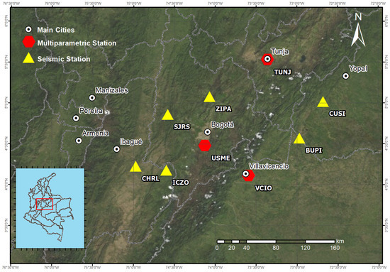
Figure 1.
Distribution of the stations of the Geophysical Network of the National University of Colombia in the central region of Colombia.
2.5.1. Sensors
The sensors used in multi-parameter stations are [26]:
- Broadband Seismometer CME 4311: Electrochemical transducer designed for permanent or portable installation. It is a robust instrument that is easy to install. In addition, it does not require maintenance, mass blocking, or leveling. This sensor offers an effective solution for installations with a noise level close to the low-noise model with a response between 1/60 and 50 Hz [27].
- Non-polarizable electrode for burial Tinker & Rasor DB-A: Copper and copper sulfate (Cu/CuSO4) electrode, non-polarizable, which allows direct exposure of copper sulfate over a large contact area. It has a shelf life of up to 10 years. Its structure is made of PVC/ABS and has a low freezing point and high evaporation point, which makes it robust for most environments. Dimensions: 7 cm in diameter, 12.2 cm high, and a weight of 896 g [28].
- Magnetometer Bartington Mag648L: Low-power, low-noise triaxial magnetometer with ±60 µT range. It has vehicular, perimeter security, and ground measurement applications [29].
Figure 2 shows the instrumental deployment corresponding to the USME station.
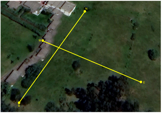
Figure 2.
Schematic representation of the location of the orthogonal dipoles, corresponding to the USME station.
2.5.2. Acquisition Hardware
The digitizer is based on a Raspberry Pi 3 CPU with 1.2 GHz processing and 2 GB of RAM, with an independent video chip. Different peripherals are integrated into it via GPIO or USB. The 24-bit Analog–Digital Converter (ADC) is connected via serial communication protocol, having eight single channels to sample up to 500 sps that can be expanded to 16 channels. To achieve time synchronization with an error of fewer than 10 μs, we use a GPS connected via asynchronous serial communication, with the possibility of an external high-gain antenna to improve the view of the sky. Data transmission is via 3G modem. The power supply is obtained using a 5 V DC source at 2.5 A that is provided using a solar panel. The maximum consumption is around 10 W. The entire system is installed in a hard box.
2.6. Data Processing
The MT data processing in this study begins by converting a time series of magnetic and electrical signals to their frequency domain (using the Fourier transform (FT)), a stacking process over a 1-h time window (it is desired to see changes in the resistivity behavior each hour), to later operate their respective components, calculate the Schmucker–Weidelt transfer function from Equation (2), and finally obtain their associated values of . This procedure was performed by developing our algorithm code in Python, which can be obtained by consulting the authors. The processing was performed following all the mathematical guidelines given in [6].
2.6.1. Time Windows
To estimate the space–time variation, particular time intervals should be defined depending on the changes to be seen. Therefore, we define three principal time windows: total window, partial window, and calculation window.
- Total window: It is the complete time interval on which to work (e.g., you want to analyze six days along which there was seismic activity: total window = 6 days);
- Partial Window: It is the time interval in which you want to see changes in the of the rocks (e.g., you want to see changes every hour: partial window = 1 h);
- Calculation window: It is the time interval over which we will calculate the Fourier Transform (FT) and, therefore, the variable used as the period () in the MT method equations (e.g., 10 s, 100 s, or 1000 s, depending on the depth of penetration to be obtained).
In this study:
- Total window: 6 days;
- Partial window: 1 h;
- Calculation window: 1000 s.
2.6.2. Apparent Resistivity Dispersion—Apparent Resistivity Curve
The parameter (), using Equations (2) and (3), will result in several dispersion points, as observed in Figure 3. Note how the figure is plotted as a function of the period () for ease of analysis (the longer the period, the greater the skin depth). After obtaining all the associated , a statistical data treatment is carried out for values of frequencies (periods) chosen in such a way that a reliable resistivity curve is obtained.
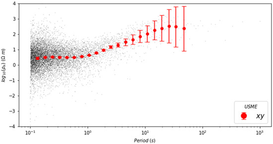
Figure 3.
Apparent resistivity dispersion as a function of the period (). The gray dots represent the raw data computed from Equation (3). The red dots represent the fitted curve used for the apparent resistivities of the partial time window (‘xy’ means HQE-HFN).
To choose the period points to be evaluated, we consider the conditions stipulated in [6]:
- The chosen periods (or frequencies) must be equally spaced on a logarithmic scale;
- Ideally, it would help to have between 6–10 frequencies per magnitude. More frequencies are unnecessary, and fewer may result in unreliable values.
Points are selected as follows:
where (sample rate = 20 Hz).
After obtaining the desired frequencies, we observe that the dispersion of the data for each point will have a Gaussian behavior, as seen in Figure 4. This allows us to find a single value associated with a single frequency/period and the corresponding standard deviation. Figure 3 shows an example of a curve obtained from fitting our dispersion data.
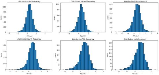
Figure 4.
Distribution of the first six frequencies chosen to represent the apparent resistivity curve.
Now that we have the curve for each hour, an map is made in the total window (days), thus allowing precise observation of the space–time changes where the target seismic event occurred.
2.6.3. Apparent-Resistivity Map
The map (Figure 5), which is obtained from our algorithm code, can be seen as a matrix of values of N rows and M columns (Equation (6)) where each column represents a 1-h time window, and each row represents each frequency/period point (N = ‘Number of point periods’ and M = ‘Number of partial windows’). Each column corresponds to the apparent resistivity-fitted curve (Figure 3); the only difference is the color assigned to each resistivity value (Figure 5).
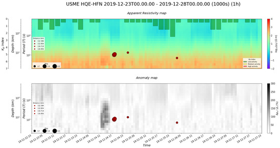
Figure 5.
Anomaly registered before the 6.0 Mw Mesetas earthquake calculating the apparent resistivity from USME HQE-HFN channels. (Format of digitized data on the time axis: year-month-day hour).
As a second option, moving on to the interpretation of the map, this can also be seen as a depth profile. Each period in each column means a different and greater depth; let us remember the relation of Equation (1), which tells us that the longer the period, the greater the skin depth (keeping in mind that this parameter also depends on the resistivity of the medium).
2.6.4. Anomaly Map
As the color map can show some anomalous behaviors at specific depths (space–time variations), sometimes this phenomenon cannot be seen clearly. Therefore, it is necessary to create an anomaly map that represents the same time interval and depth ranges.
The values of the anomaly map (shown in the lower part of Figure 5) are the result of finding how anomalous each value of the map is, that is, quantifying how much each one varies according to the average of the total window. First, the average value of the window is found, which will be a column of N rows resulting from the average resistivity for each period:
Starting from the matrix, which represents the apparent resistivity map (left part), then () we average each row (middle part), which is equivalent (=) to an average value corresponding to each row (period); we get:
thus, obtaining an average value for each period.
Finally, each value of the initial apparent resistivity matrix () is operated with its corresponding average () as follows:
to obtain a percentage of the anomaly. This value means how different each value () is from the average () of the total window, e.g., getting an anomaly value of 300% means that we have a value three times greater than the average.
By obtaining all values of the anomalies, we will be able to plot a map with the same dimensions as the map. This map is presented in grayscale (Figure 5) and allows us to see more clearly the area where an anomalous resistivity value occurs according to the average value of the total window.
3. Results and Discussion
Considering several variables such as solar activity, , and associated anomalies, the results of this study provide visual information for interpreting in a simpler and more complete way. Figure 5 shows the space–time changes of the for the USME station during the time interval when the Mesetas earthquake occurred (Mw6.0, Lon = 74.184° W, Lat = 3.462° N, H = 13 km-depth, 24 December 2019, UTC 19:03:55) and its associated aftershocks.
Solar activity (Kp index): Average low solar activity (<2). A behavior without significant variation is observed throughout the time window, except for a small peak of 2.5 on 26 December.
Apparent resistivity: The variation of the depending on the depth H can be classified into three ranges of periods (Table 2):
Table 2.
Variations of the depending on the depth H.
Associated anomalies: There is a clear anomaly presented 11–16 h before 24 January (Table 3):
Table 3.
anomaly depending on the depth H.
Figure 6 shows the curves found for a partial window before, during, and after the anomaly found (black: curve before the anomaly, red: curve during the anomaly, blue: curve after the anomaly). A slight increase can be observed in the periods (depths) involved in the red curve, which means that at this specific time interval, there was a slight increase in the of the subsurface between the periods shown in Figure 5. Geologically speaking, and because resistivity in rocks largely depends on their saturation fluids, this anomaly can be related to a momentary migration of fluids in the rock due to stresses produced in the mainshock, and then a return to initial equilibrium.
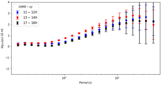
Figure 6.
Comparison between three apparent resistivity curves, each corresponding to a different hour interval of December 24 (UTC). The red curve represents the time when the anomaly is observed.
The same procedure was done for the TUNJ station (also RSUNAL station) to rule out the idea that the found anomaly simply meant instrumental noise at the station. The results are illustrated in Figure 7. In this case, we see more anomalies, which are interpreted as external noise due to their periodicity. It is observed that there is also a disturbance of lesser magnitude in a depth range (periods) close to the depth of the seismic event, even if the event occurred at a greater distance from the station (~250 km).
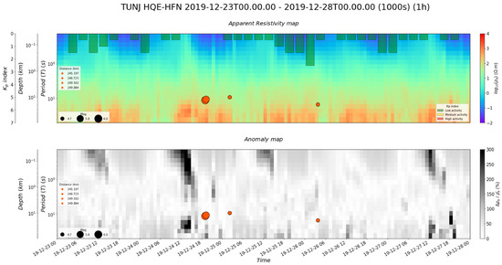
Figure 7.
Anomalies registered at TUNJ station for the same Mesetas events.
4. Conclusions
The particularities identified in the case of the earthquakes in Mesetas yield suggestive results of an anomaly in the subsoil eight hours before the first recorded seismic event (6.0 Mw), a duration 4–5 h from the start of the anomaly and within a range of periods between 1–30 s (depths between 1.5–40 km). It is also shown that this disturbance does not correspond to instrumental noise since it also exists and is registered at the TUNJ station. The origin of these anomalies may be associated with the migration of fluids due to the change in the stress regime before, during, and after the earthquake. We hypothesize that before the occurrence of an earthquake, the stress field generates pore pressure gradients, promoting alterations in fluid migration that change the resistivity of the upper crust.
The anomalies detected and observed at the USME multi-parameter station do not show a direct and causal relationship with seismic events of less than 5.8 Mw or distances greater than 120 km. However, since the notable anomalies in the designed algorithm must exceed 100% (double the average value), it is not ruled out that there are patterns of changes in the of the subsoil of lower percentages related to these events. For these cases, we have used a minor anomaly scale.
Author Contributions
Conceptualization, C.A.V., J.S.G., J.J.G., J.M.S. and A.C.; Methodology, C.A.V., J.S.G. and J.J.G.; Software, J.S.G. and J.J.G.; Validation, J.S.G. and J.J.G.; Formal analysis, C.A.V., J.S.G. and A.C.; Writing, C.A.V., J.S.G. and A.C.; All authors have read and agreed to the published version of the manuscript.
Funding
Colombia Móvil–TIGO (Colombia) contributed with the data transmission, through mobile network, from remote sites to the data processing center, located at the National University of Colombia at Bogota.
Institutional Review Board Statement
Not applicable.
Informed Consent Statement
Not applicable.
Data Availability Statement
Once the paper is approved, the dataset will be openly available.
Acknowledgments
The authors want to express their gratitude to the Universidad Nacional Colombia at Bogotá and Universidad Antonio Nariño at Bogotá. Without their support and mutual collaboration, the permanent operation of the multi-parameter network would not be possible. The authors thank the Special Issue Editors (Guest Editors), for their patience, as well as two anonymous reviewers, for their valuable comments and suggestions.
Conflicts of Interest
The authors declare no conflict of interest.
References
- Du, X.-B.; Xue, S.-Z.; Hao, Z.; Zhang, S.-Z. On the relation of moderate-short term anomaly of earth resistivity to earthquake. Acta Seism. Sin. 2000, 13, 393–403. [Google Scholar] [CrossRef]
- Du, X.-B.; Li, N.; Ye, Q.; Ma, Z.-H.; Yan, R. A Possible Reason for the Anisotropic Changes in Apparent Resistivity Near the Focal Region of Strong Earthquake. Chin. J. Geophys. 2007, 50, 1555–1565. [Google Scholar] [CrossRef]
- Fan, Y.-Y.; Du, X.-B.; Jacques, Z.; Tan, D.-C.; An, Z.-H.; Chen, J.-Y.; Zheng, G.-L.; Liu, J.; Xie, T. The Electromagnetic Phenomena Before theMs8.0 Wenchuan Earthquake. Chin. J. Geophys. 2010, 53, 997–1010. [Google Scholar] [CrossRef]
- Liu, J.; Du, X.B.; Zlotnicki, J.; Fan, Y.Y.; An, Z.H.; Xie, T.; Zheng, G.L.; Tan, D.C.; Chen, J.Y. The changes of the ground and ionosphere electric/magnetic fields before several great earthquakes. Chin. J. Geophys. 2011, 54, 2885–2897. [Google Scholar] [CrossRef]
- Cagniard, L. Basic Theory of the Magneto Telluric Method of Geophysical Prospecting. Geophysics 1953, 18, 605–635. [Google Scholar] [CrossRef]
- Simpson, F.; Bahr, K. Practical Magnetotellurics; Cambridge University Press: Cambridge, UK, 2005. [Google Scholar] [CrossRef]
- Uyeda, S.; Nagao, T.; Kamogawa, M. Short-term earthquake prediction: Current status of seismo-electromagnetics. Tectonophysics 2008, 470, 205–213. [Google Scholar] [CrossRef]
- Uyeda, S.; Nagao, T.; Kamogawa, M. Earthquake Precursors and Prediction. In Encyclopedia of Solid Earth Geophysics; Gupta, H.K., Ed.; Encyclopedia of Earth Sciences Series; Springer: Dordrecht, The Netherlands, 2011. [Google Scholar]
- Sarlis, N.V.; Skordas, E.S.; Varotsos, P.A. Natural Time Analysis: Results Related to Two Earthquakes in Greece during 2019. In Proceedings of the 2nd International Electronic Conference on Geosciences, Online, 8–15 June 2019; Available online: https://iecg2019.sciforum.net/ (accessed on 26 January 2023).
- Cicerone, R.D.; Ebel, J.E.; Britton, J. A systematic compilation of earthquake precursors. Tectonophysics 2009, 476, 371–396. [Google Scholar] [CrossRef]
- Varotsos, P.A.; Sarlis, N.V.; Skordas, E.S.; Lazaridou, M.S. Electric pulses some minutes before earthquake occurrences. Appl. Phys. Lett. 2007, 90, 064104. [Google Scholar] [CrossRef]
- Varotsos, P.; Sarlis, N.; Skordas, E.; Lazaridou, M. Additional evidence on some relationship between Seismic Electric Signals (SES) and earthqueake focal mechanism. Tectonophysics 2006, 412, 279–288. [Google Scholar] [CrossRef]
- Johnston, M.J.S. Review of Electric and Magnetic Fields Accompanying Seismic and Volcanic Activity. Surv. Geophys. 1997, 18, 441–476. [Google Scholar] [CrossRef]
- Shrivastava, A. Are pre-seismic ULF electromagnetic emissions considered as a reliable diagnostics for earthquake prediction? Curr. Sci. 2014, 107, 596–600. [Google Scholar]
- Petraki, E.; Nikolopoulos, D.; Nomicos, C.; Stonham, J.; Cantzos, D.; Yannakopoulos, P.; Kottou, S. Electromagnetic pre-earthquake precursors: Mechanisms, data and models-a review. J. Earth Sci. Clim. Chang. 2015, 6, 250. [Google Scholar]
- Stanica, D.; Stanica, D.A. Anomalous pre-seismic behavior of the electromagnetic normalized functions related to the intermediate depth earthquakes occurred in Vrancea zone, Romania. Nat. Hazards Earth Syst. Sci. 2011, 11, 3151–3156. [Google Scholar] [CrossRef]
- Zhang, X.; Shen, X. Electromagnetic Anomalies around the Wenchuan earthquake and their relationship with earthquake preparation. Int. J. Geophys. 2011, 2011, 904132. [Google Scholar] [CrossRef]
- Koulouras, G.; Balasis, G.; Kiourktsidis, I.; Nannos, E.; Kontakos, K.; Stonham, J.; Ruzhin, Y.; Eftaxias, K.; Cavouras, D.; Nomicos, C. Discrimination between pre-seismic electromagnetic anomalies and solar activity effects. Phys. Scr. 2009, 79, 045901. [Google Scholar] [CrossRef]
- Febriani, F.; Han, P.; Yoshino, C.; Hattori, K.; Nurdiyanto, B.; Effendi, N.; Maulana, I.; Gaffar, E.Z. Ultra low frequency (ULF) electromagnetic anomalies associated with large earthquakes in Java Island, Indonesia by using wavelet transform and detrended fluctuation analysis. Nat. Hazards Earth Syst. Sci. 2014, 14, 789–798. [Google Scholar] [CrossRef]
- Lowrie, W. Fundamentals of Geophysics, 2nd ed.; Cambridge University Press: New York, NY, USA, 2007; 393p. [Google Scholar]
- Chave, A.; Jones, A. The Magnetotelluric Method, Theory and Practice; Cambridge University Press: Cambridge, UK, 2012. [Google Scholar] [CrossRef]
- Weidelt, P. The inverse problem of geomagnetic induction. Z. Geophys. 1972, 38, 257–289. [Google Scholar] [CrossRef]
- Schmucker, U. Regional induction studies: A review of methods and results. Phys. Earth Planet. Inter. 1973, 7, 365–378. [Google Scholar] [CrossRef]
- NOAA (National Oceanic and Atmospheric Administration). Available online: https://www.swpc.noaa.gov/products/planetary-k-index. (accessed on 19 December 2022).
- Vargas, C.A.; Caneva, A.; Monsalve, H.; Salcedo, E.; Mora, H. Geophysical Networks in Colombia. Seism. Res. Lett. 2018, 89, 440–445. [Google Scholar] [CrossRef]
- Fino, J.M.S.; Caneva, A.; Jiménez, C.A.V.; Ochoa, L.H. Electrical and magnetic data time series’ observations as an approach to identify the seismic activity of non-anthropic origin. Earth Sci. Res. J. 2021, 25, 297–307. [Google Scholar] [CrossRef]
- CME. Broadband Seismometer Model CME-4111. Available online: http://r-sensors.ru/en/products/digital_seismometers_eng/cme-4211nd-eng/ (accessed on 19 December 2022).
- Tinker-Rasor. Direct Burial—Tinker & Rasor. 2021. Available online: https://www.tinker-rasor.com/direct-burial (accessed on 19 December 2022).
- Bartington Instruments. Mag648 & Mag649 Low Power Three-Axis Magnetic Field Sensors. Available online: https://www.bartington.com/products/low-power-magnetometers/mag648-649/ (accessed on 19 December 2022).


Disclaimer/Publisher’s Note: The statements, opinions and data contained in all publications are solely those of the individual author(s) and contributor(s) and not of MDPI and/or the editor(s). MDPI and/or the editor(s) disclaim responsibility for any injury to people or property resulting from any ideas, methods, instructions or products referred to in the content. |
© 2023 by the authors. Licensee MDPI, Basel, Switzerland. This article is an open access article distributed under the terms and conditions of the Creative Commons Attribution (CC BY) license (https://creativecommons.org/licenses/by/4.0/).