Monocular 3D Object Detection Based on Pseudo Multimodal Information Extraction and Keypoint Estimation

Abstract

Three-dimensional object detection is an essential and fundamental task in the field of computer vision which can be widely used in various scenarios such as autonomous driving and visual navigation. In view of the current insufficient utilization of image information in current monocular camera-based 3D object detection algorithms, we propose a monocular 3D object detection algorithm based on pseudo-multimodal information extraction and keypoint estimation. We utilize the original image to generate pseudo-lidar and a bird’s-eye view, and then feed the fused data of the original image and pseudo-lidar to the keypoint-based network for an initial 3D box estimation, finally using the bird’s-eye view to refine the initial 3D box. The experimental performance of our method exceeds state-of-the-art algorithms under the evaluation criteria of 3D object detection and localization on the KITTI dataset, achieving the best experimental performance so far.

1. Introduction

Three-dimensional object detection is an essential and important environmental perception task in autonomous driving which can provide the precise location of the surroundings within a certain distance for a moving car. In recent years, 3D object detection algorithms based on lidar [1,2,3] or stereo cameras [4,5,6] have achieved an excellent detection performance by virtue of their direct or indirect depth information, however, due to the inherent high cost or low robustness to adverse weather conditions of lidar-based detectors and cumbersome online calibration problems of stereo cameras, the application and development of these two detection methods have been limited.

On the contrary, the research of monocular 3D object detection algorithms [7,8,9,10,11,12,13] has become a promising research direction by virtue of its advantages of a low cost and easy operation. Monocular 3D object detection means to classify and locate each object within a certain distance in a surrounding environment by only a single camera; the goal of monocular 3D object detection is to estimate a minimal 3D bounding box tightly wrapping the object. In KITTI [14], the 3D bounding box can be parameterized as follows: (i) the object’s position (x, y, z), meaning the position of the center point of the 3D box in the camera coordinate system (unit: meters); (ii) the object’s dimensions (l, w, h), representing the length, width, and height of the 3D bounding box (in meters); and (iii) the object’s angle, which is the orientation angle of the 3D box. The biggest challenge in improving the performance of a 3D object detection algorithm is how to accurately estimate the object’s position (x, y, z), among which the estimation of the depth value is the most important. Therefore, how to obtain accurate depth information is an import role of monocular 3D object detection. Previous methods [7,9,15,16] perform 3D object detection by virtue of geometric constraints between 2D images and 3D objects, but their experimental performances are worse on account of the lack of direct or indirect depth information. For example, Deep3D box [16] performs 3D object detection by right of strong geometric constraint information from the 2D bounding box, and the estimated 3D bounding box closely fits the 2D bounding box. The performance of such algorithms largely depends on the precision of 2D object detection because of the strong dependency between 3D object detection and 2D detection. Other methods [17,18,19] generate pseudo-lidar by introducing extra depth information and utilize existing mature lidar-based detection framework to perform 3D object detection, whereas such algorithms are computationally inefficient because it has to deal with a huge number of pseudo-lidar points.

The paper proposes a monocular 3D object detection algorithm based on pseudo-multimodal information extraction and keypoint estimation. First, we utilize mature 2D detection framework to accomplish 2D object detection. Second, we fuse the two different modalities: the 2D region of interest and the region pseudo-lidar to perform the keypoint-based initial 3D object detection. Finally, we utilize the bird’s-eye view features generated by the pseudo-lidar to refine the initial 3D box, consequently achieving the purpose of extracting three different modal information of the original image for 3D object detection.

In summary, our main contributions are as follows:

1. We propose a monocular 3D object detection algorithm based on pseudo-multimodal information extraction and keypoint estimation.

2. It is the first time that multi-modal information has been extracted from an original image for 3D object detection, which makes the extracted information more comprehensive and richer.

3. Our method achieves a state-of-the-art experimental performance on the KITTI dataset.

2. Related Work

This part briefly introduces the latest research progress of 3D object detection algorithms based on lidar, stereo cameras, and the monocular camera.

2.1. LiDAR-Based Methods

Lidar-based methods [1,2,3,10,11,20,21,22,23] represent the 3D object detection algorithms with the best performance at the moment; these methods deal with lidar points in different ways. For example, VoxelNet [20] and SECOND [21] convert the point cloud to voxels for 3D detection and MV3D [13], PIXOR [22], and AVOD [11] project the point cloud to the front view or bird’s-eye view for 3D detection. PointPillar [1] directly generates pseudo images from the point cloud and then utilizes 2D methods to process the pseudo images. These methods will cause serious quantization errors in the process of converting data types. Point RCNN [3] extracts an original point cloud feature and generates point cloud-based region proposals on the original point cloud. IA-SSD [2] utilizes two kinds of learnable task-oriented and instance-aware down sampling strategies to hierarchically select the foreground points belonging to objects of interest in the original point cloud.

2.2. Stereo-Based Methods

The performance of 3D object detection algorithms based on stereo cameras [4,5,6,24,25,26,27,28,29] has also been greatly improved recently. For example, Stereo R-CNN [5] utilizes the dual RPN structure to fuse the stereo features and construct the stereo geometric relationship for 3D object detection and refines the 3D bounding box by the pixel-by-pixel matching of the left and right images. Object-Centric [6] only performs stereo matching on the object of interest in the stereo images, solving the problem of a pixel imbalance between far and near objects. DSGN [4] performs 3D object detection by constructing a derivable 3D geometry volume, thus narrowing the gap between image-based methods and LiDAR-based methods. Pseudo-lidar++ [25] utilizes sparse lidar to correct the depth of the pseudo-lidar point cloud generated based on stereo images, thereby improving the accuracy of 3D object detection without increasing the cost significantly. PLUMENet [24] constructs a pseudo-lidar feature volume directly in 3D space for both the depth estimation and 3D object detection. The stereo cameras can provide more abundant information than the monocular camera and include the depth information required for positioning, but the installation and setting requirements of stereo cameras are relatively high. In comparison, our monocular camera-based 3D object detection is more flexible and less expensive.

2.3. Monocular-Based Methods

The cost of lidar-based 3D object detection algorithms is relatively high and the installation of stereo cameras is more complicated considering the calibration problem between the two cameras. Therefore, monocular 3D object detection [7,12,13,17,21,30,31,32,33] is gaining popularity. In general, monocular 3D object detection can be mainly divided into two types: keypoint regression-based methods [33,34,35] and depth maps-based methods [10,18,30,36,37].

2.3.1. Keypoint-Based Methods

Keypoint-based monocular 3D object detection such as CenterNet [35], SMOKE [34], and MonoCon [33] regard the object as a key point for estimation, which reduces the difficulty of 3D object detection. These methods usually use a lightweight convolutional neural network (CNN) for the features’ extraction; therefore, the algorithm’s structure is simple and the computational efficiency is relatively high. Referring to the key-point detection technology in human pose estimation, some other algorithms construct the geometric constraints between specific keypoints and 2D objects for 3D object detection. Gupta [38] solved the 3D localization problem by predicting the 2D projection of the bottom center of the 3D bounding box and uses a lookup table-based approach to re-project the bottom center of the 3D bounding box in 3D space. RTM3D [8] estimates nine keypoints of the 3D bounding box and then uses the geometric relationship between 2D and 3D views to recover the key information.

2.3.2. Depth-Based Methods

Most of these algorithms utilize the depth estimation network to generate a depth map, which can be directly used as an input or combined with the original image or converted into pseudo-lidar for 3D object detection. M3D-RPN [30] and D4LCN [18] use depth maps to generate depth-aware convolutions to extract the key information from 2D images more flexibly and accurately. Xinshuo Weng [10] and MultiFusion [36] make use of the depth map to generate pseudo-lidar information for 3D object detection. There are also some depth-based algorithms, such as CaDDN [37], which assigns discrete depth buckets to each pixel position to predict the probability that it belongs to, avoiding the network’s excessive dependence on the accuracy of the depth estimation.

3. Methods

The method we propose is mainly aimed at the situation of using a single camera to perform monocular 3D object detection in the autonomous driving environment. The 3D bounding box wrapping tightly around the object can be parameterized as $(\mathrm{x},y,z,l,w,h,\theta )$. $(x,y,z)$ represents the position of the object, (l, w, h) represents the length, width, and height of the object, and $\theta$ represents the rotation angle of the object relative to the Y-axis in the camera coordinate system. Consistent with KITTI, we assume that the rotation angle of the object relative to the X-axis and Z-axis is zero and the camera internal parameter matrix K is known.

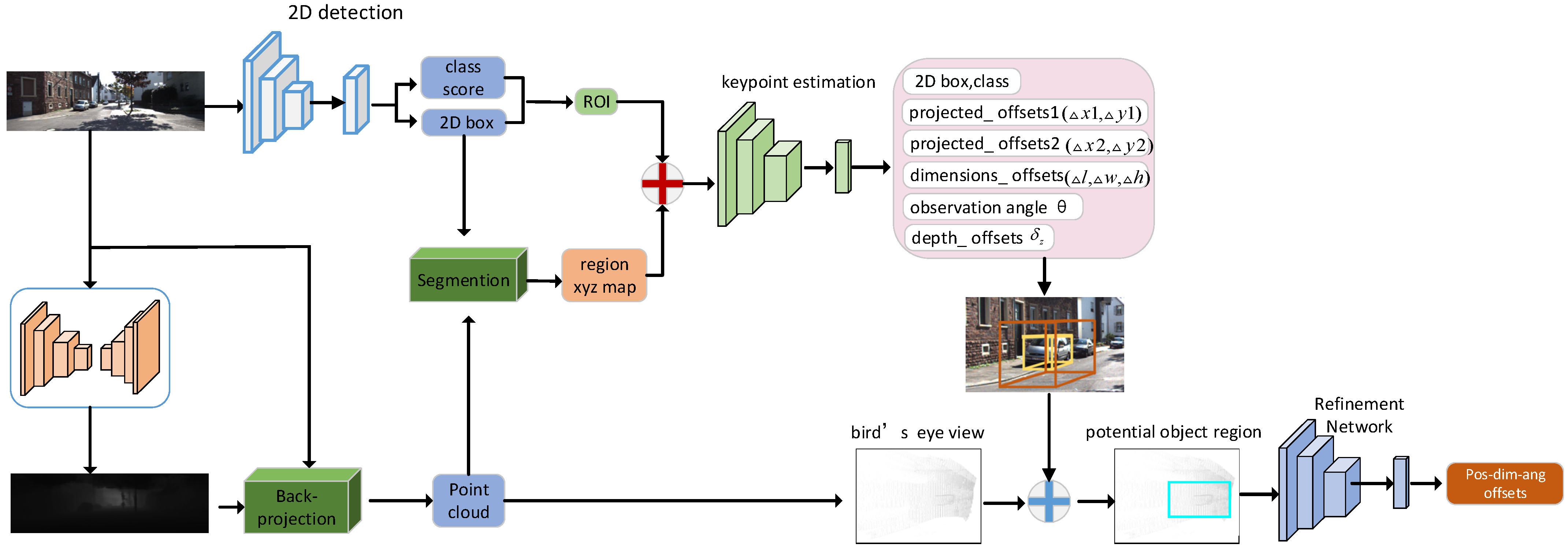
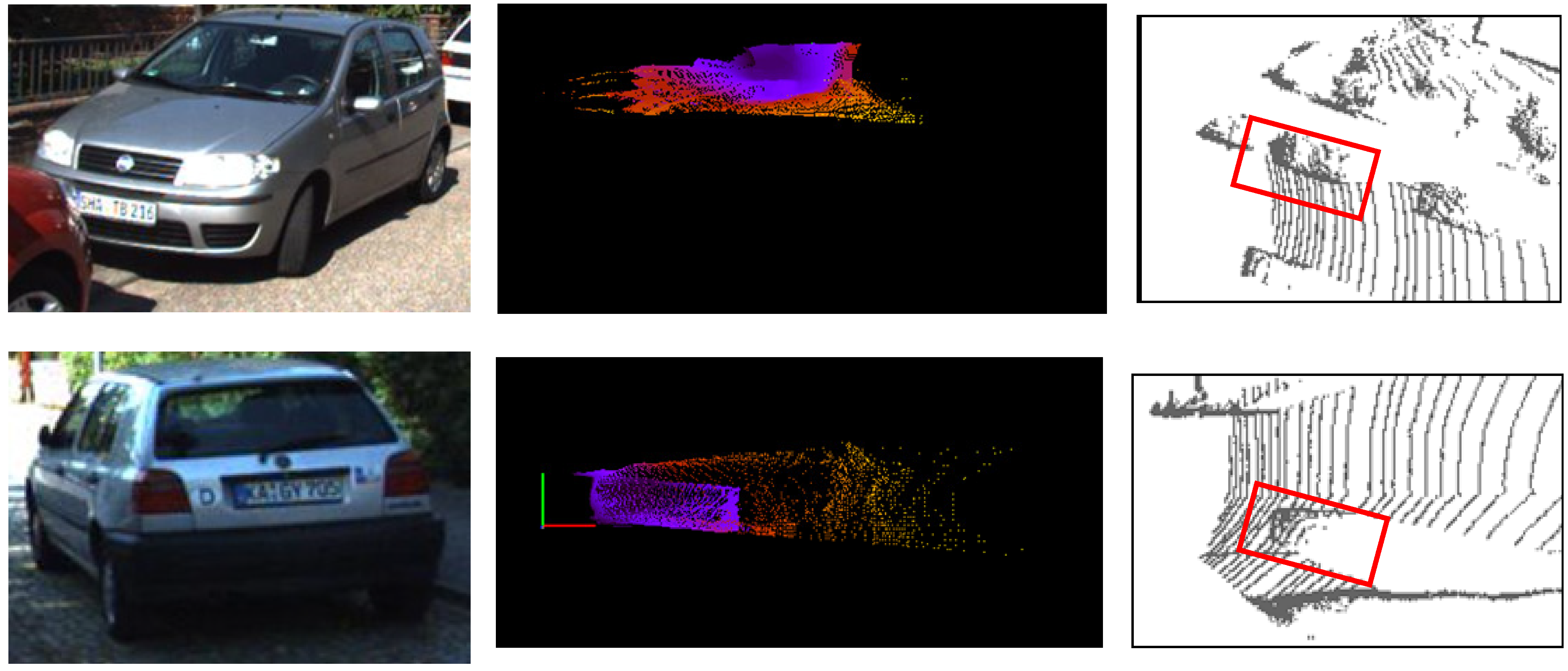
Our algorithm framework is shown in Figure 1. In the first place, we perform 2D detection and depth estimation to obtain the 2D region of interest and depth map. Then, we fuse the 2D region of interest and region pseudo-lidar generated from the depth map and also feed the fused data to the keypoint estimation network for the estimation of the coarse initial 3D box. For the purpose of auxiliary learning, we again estimate the 2D parameters when performing 3D object detection, hoping to utilize the high-precision characteristics of 2D detection to help the learning of the 3D parameters. Finally, we use the bird’s-eye view features generated from the pseudo-lidar information to refine the initial 3D box. The visualization illustration of the original image, pseudo-lidar, and bird’s-eye view used in our algorithm is shown in Figure 2.

3.1. Estimation of the Initial 3D Box

3.1.1. Generation of the 2D Roi

In order to complete the 3D object detection, we primarily need to perform 2D object detection to generate the 2D region of interest. We adopt the multi-scale detection framework of MS-CNN [39] as our 2D detection framework, which is conducive to a more accurate detection of distant objects and smaller objects in the near distance.

3.1.2. Generation of the Region Pseudo-Lidar

Directly utilizing a 2D image for 3D object detection will result in a low performance due to the lack of depth information. Therefore, we choose to fuse the stereoscopic information of the pseudo-lidar into the 2D image’s features to improve the precision of the 3D detection. In order to generate the region pseudo-lidar, we firstly utilize a mature depth estimator DORN [40] to generate a depth map and convert the depth map to the dense pseudo-lidar. PatchNet [12] transforms the pseudo-lidar point cloud into an XYZ three-channel model and utilizes a 2D CNN to extract the pseudo-lidar points’ features and estimate the 3D parameters, which simplifies the network’s structure and reduces the difficulty of training. In this paper, inspired by PatchNet [12], we correspond the pseudo-lidar points to each pixel in the 2D image and rearrange them in the form of three-channel XYZ. Finally, we project the 2D detection box onto the pseudo-lidar (XYZ map) to filter out a large number of background point clouds and we obtain a region pseudo-lidar of the same size as the 2D detection box.

3.1.3. Fusion of Different Modal Information

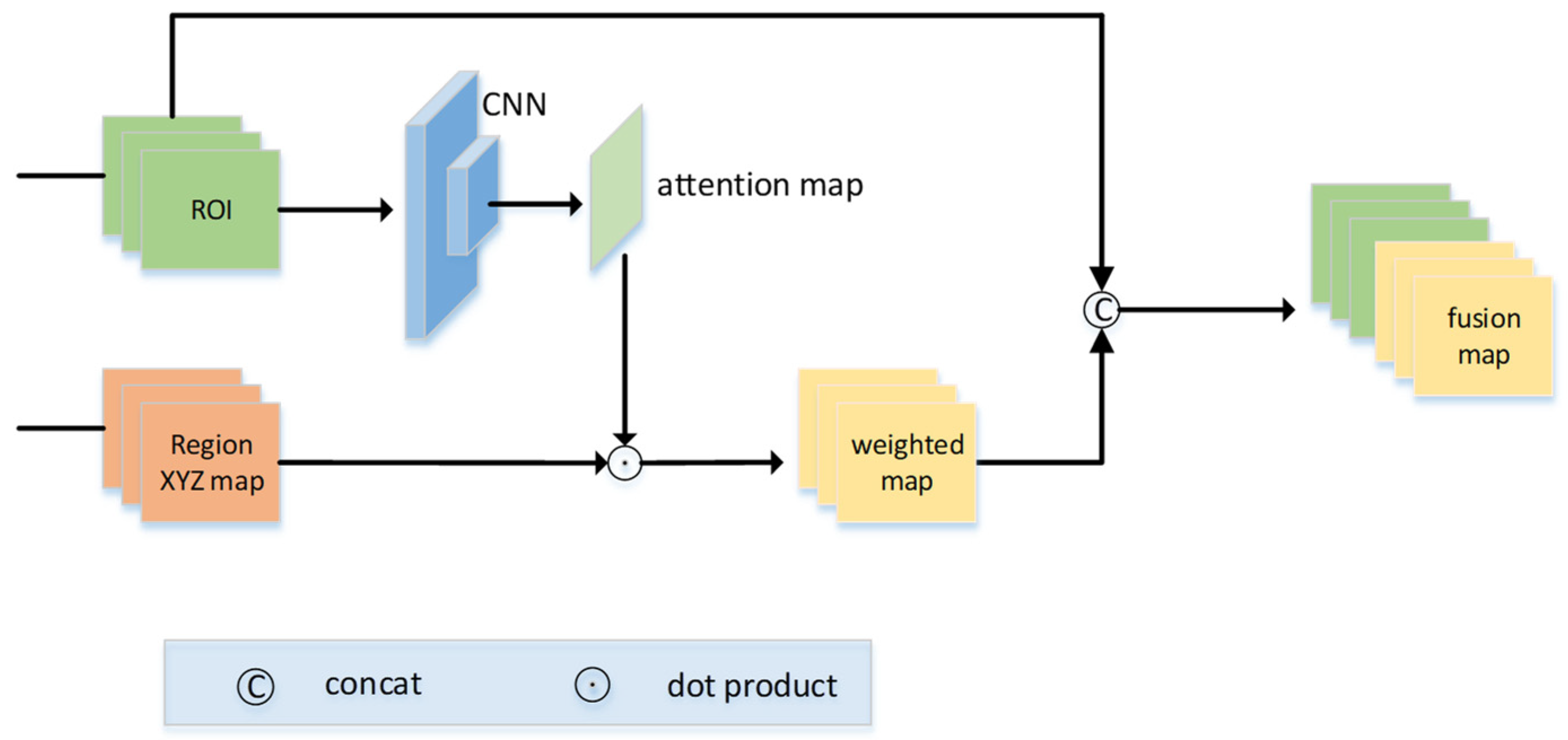
The value at each pixel position of the 2D region of interest represents the RGB value of the color image and the value at each position of the regional pseudo-lidar represents the physical position of the pixel in the 3D space. It is difficult to achieve a good experimental performance by adding together these two-modal data for 3D object detection. AM3D [17] uses the attention map generated by the pseudo-lidar to selectively incorporate useful RGB image information into the position information of the pseudo-lidar. Considering that the pseudo-lidar generated by the 2D image has a certain error, the process of utilizing the pseudo-lidar to generate the attention map will amplify this error. Therefore, we design the following attention mechanism shown in Figure 3. Primarily, we feed the region of interest to a two-layer CNN to generate an attention map and perform a dot product between the attention map and the region pseudo-lidar to obtain a weighted region pseudo-lidar. Then, we superimpose the weighted region pseudo-lidar and the 2D region of interest on the channel to complete the fusion of two different modal information. The operation of the point product between the attention map and the regional pseudo-lidar promotes a competitive mechanism between the values of the region pseudo-lidar, encouraging the values at important positions and suppressing the values at unimportant positions, which can highlight the more important position. The mechanism helps the two-modal information to be more fully fused so as to better perform subsequent initial 3D object detection. Compared with AM3D [17], our attention map is derived from the more accurate 2D region of interest rather than the pseudo-lidar with a large error, which reduces the source of error and is beneficial to improving the precision of the 3D object detection. Considering the subsequent feature extraction problem of pseudo-lidar, AM3D [17], Frustum Points [41], Pseudo-Lidar [19], etc., directly use the existing lidar-based detection framework for 3D object detection. Most of these algorithms have high memory requirements and time-consuming training. In this paper, we use a lightweight two-dimensional convolutional neural network to process the pseudo-lidar fused with image information in the image mode. The convolutional neural network has a simple structure and short training time. The computing power and storage requirements are relatively low, which greatly improves the detection speed without reducing the detection accuracy.

3.1.4. Keypoint Estimation

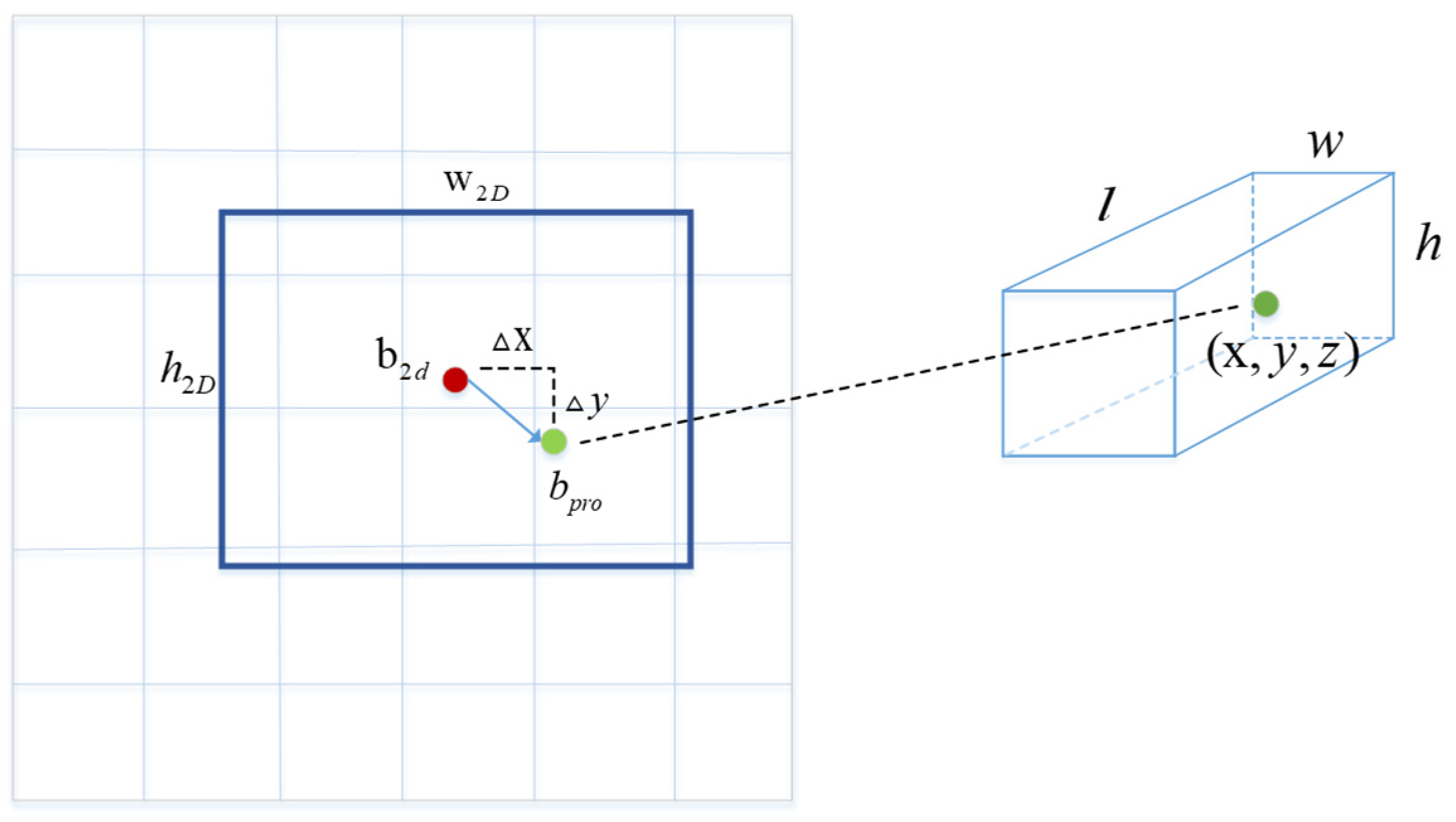
If we directly perform 3D parameters estimation using the fused feature, that is directly perform 3D object detection in 3D space, the search range is too large and the cost is too high. Considering that the projection point of the 3D box is relatively close to the center point of the 2D box, as shown in Figure 4, the red point is the center point of the 2D box and the green point is the projection point of the 3D box. Therefore, we estimate the projection point of the 3D box based on the center point of the 2D box; that is to say we regard the projection point as a key point for estimation and then back-project the projection point to 3D space to obtain the center point coordinates of the 3D box.

The relationship between the projection point of the 3D box $b_{pro}(x_{pro},y_{pro})$ and the center point of the 2D box ${\mathrm{b}}_{2d}(x_{2d},y_{2d})$ is as follows.

$$b_{pro}(x_{pro},y_{pro})=b_{2d}(x_{2d},y_{2d})+(△x,△y)$$

(1)

In the experiment, it was found that when estimating the offsets between the projection point of the 3D box and the center point of the 2D box, the experimental performance of carrying out twice offsets estimations better than the experimental performance of carrying out once offsets estimation. That is because we perform the offsets loss calculation twice, which increases the constraints and make the keypoint estimation more accurately. Thus, our keypoint estimation is designed according to the following formula:

$$b_{pro}(x_{pro},y_{pro})=b_{2d}(x_{2d},y_{2d})+(△x_1,△y_1)+(△x_2,△y_2)$$

(2)

An important part of the keypoint estimation is the generation of keypoint labels $b_{pro}^{gt}(x_{pro}^{gt},y_{pro}^{gt})$. For each object, we project the ground truth of the center point of the 3D box to the image plane through the known camera internal parameter matrix K, and then obtain the label of the key point. The formula is as follows:

$$z_{3d}^{gt}{b}_{pro}^{gt}(x_{pro}^{gt},y_{pro}^{gt})=K{B}_{3d}^{gt}(x_{3d}^{gt},y_{3d}^{gt},z_{3d}^{gt})\begin{array}{ccc}& & \end{array}$$

$$\left[\begin{array}{c}{z}_{3d}^{gt}\cdot x_{pro}^{gt}\\ z_{3d}^{gt}\cdot {\mathrm{y}}_{pro}^{gt}\\ z_{3d}^{gt}\end{array}\right]=K\cdot \left[\begin{array}{c}{z}_{3d}^{gt}\\ {\mathrm{y}}_{3d}^{gt}\\ z_{3d}^{gt}\end{array}\right]$$

(3)

Knowing the camera internal parameter matrix K, the projection formula for the center point of the 3D box $B_{3d}(x,y,z)$ projected onto the image plane to obtain the 2D projection point $b_{pro}(x_{pro},y_{pro})$ is as follows.

$$z\cdot b_{pro}(x_{pro},y_{pro})=K\cdot B_{3d}(x,y,z)\begin{array}{ccc}& & \end{array}$$

$$\left[\begin{array}{c}z\cdot x_{pro}^{}\\ z\cdot {\mathrm{y}}_{pro}^{}\\ z\end{array}\right]=K\cdot \left[\begin{array}{c}x\\ y\\ z\end{array}\right],K=\left[\begin{array}{ccc}{f}_x& 0& c_x\\ 0& f_y& c_y\\ 0& 0& 1\end{array}\right]$$

(4)

where $f_x$ and $f_{\mathrm{y}}$ are the focal lengths of the x-axis and y-axis directions and $c_x$ and $c_y$ are the projections of the camera’s optical center on the image plane.

According to the projection Formula (3), when the projection point $b_{pro}(x_{pro},y_{pro})$ is back-projected to the 3D space to obtain the center point coordinate of the 3D box, the back-projection formula is as follows:

$$B_{3d}(x,y,z)=K^{-1}\cdot z\cdot b_{pro}(x_{pro},y_{pro})\begin{array}{ccc}& & \end{array}$$

$$\left[\begin{array}{c}x\\ y\\ z\end{array}\right]=K^{-1}\cdot \mathrm{z}\cdot \left[\begin{array}{c}{x}_{pro}\\ y_{pro}\\ 1\end{array}\right]=K^{-1}\cdot \mathrm{z}\cdot \left[\begin{array}{c}{x}_{2d}+△x_1+△x_2\\ y_{2d}+△y_1+△y_2\\ 1\end{array}\right]$$

(5)

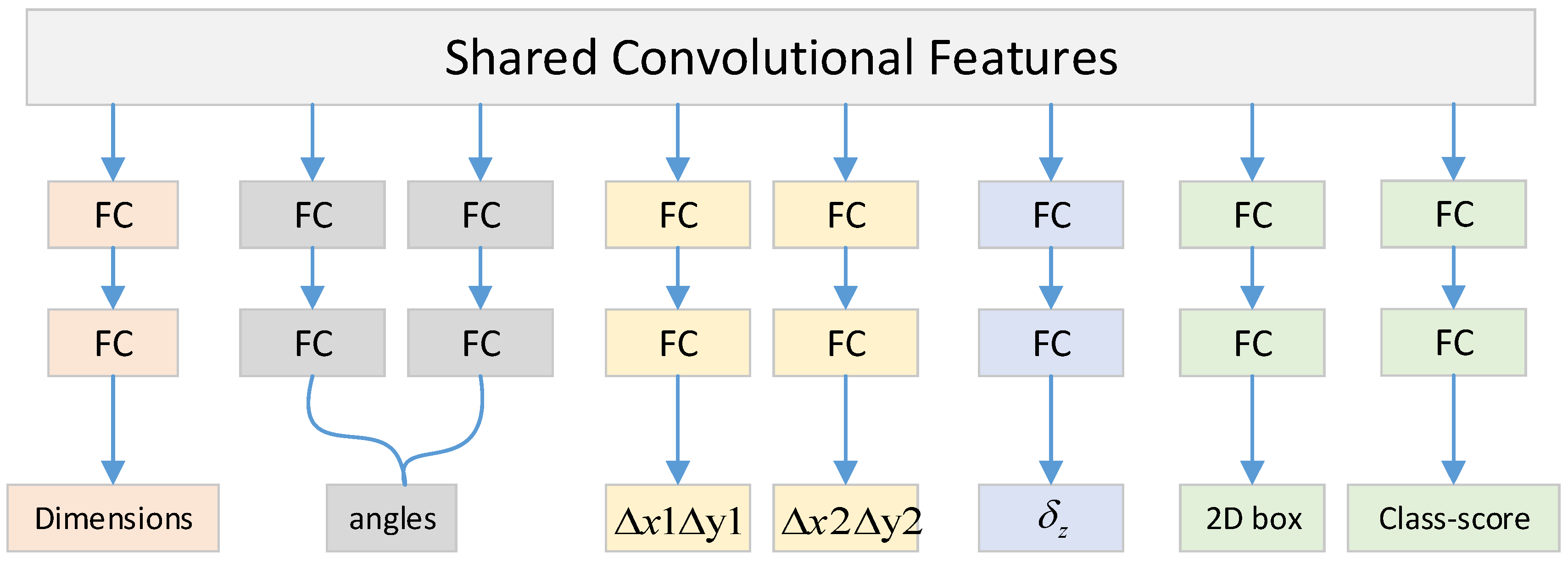
It can be seen from Formula (4) that in order to obtain the center point coordinates of the 3D box, we need to estimate not only the position of the projection point but also the depth value of the center point of the 3D box. As shown in Figure 5, at the end of the keypoint estimation network, there are three fully connected layers, after which is the detection head corresponding to the 3D box’s parameters. The depth detection head branch estimates a depth offset ${\delta }_z$ which is combined with the depth adjustment parameters ${\mu }_{\mathrm{z}}$ and ${\sigma }_z$ (${\mu }_{\mathrm{z}}$ and ${\sigma }_z$ are known parameters obtained from statistics of the same category in the dataset) to obtain the depth of the center of the 3D box by the following formula:

$$z={\mu }_z+{\delta }_z{\sigma }_z$$

(6)

After obtaining the depth value of the center point of the 3D box, the center point coordinates of the 3D box in the camera coordinate system can be obtained through the back-projection Formula (4).

3.1.5. Estimation of Angle and Dimension

As shown in Figure 5, in addition to regress the center position of the 3D box, we also need to regress the dimension and angle. The dimension regression branch estimates the dimension offsets $({\delta }_l,{\delta }_w,{\delta }_h)$ of the 3D box. Knowing the average value $(\overline{l},\overline{w},\overline{h})$ of the dimension of the 3D box in the dataset, the dimension of the 3D box can be calculated by the following formulas:

$$\left[\begin{array}{c}l\\ w\\ h\end{array}\right]=\left[\begin{array}{c}\overline{l}\cdot e^{{\delta }_1}\\ \overline{w}\cdot e^{{\delta }_w}\\ \overline{h}\cdot e^{{\delta }_h}\end{array}\right]$$

(7)

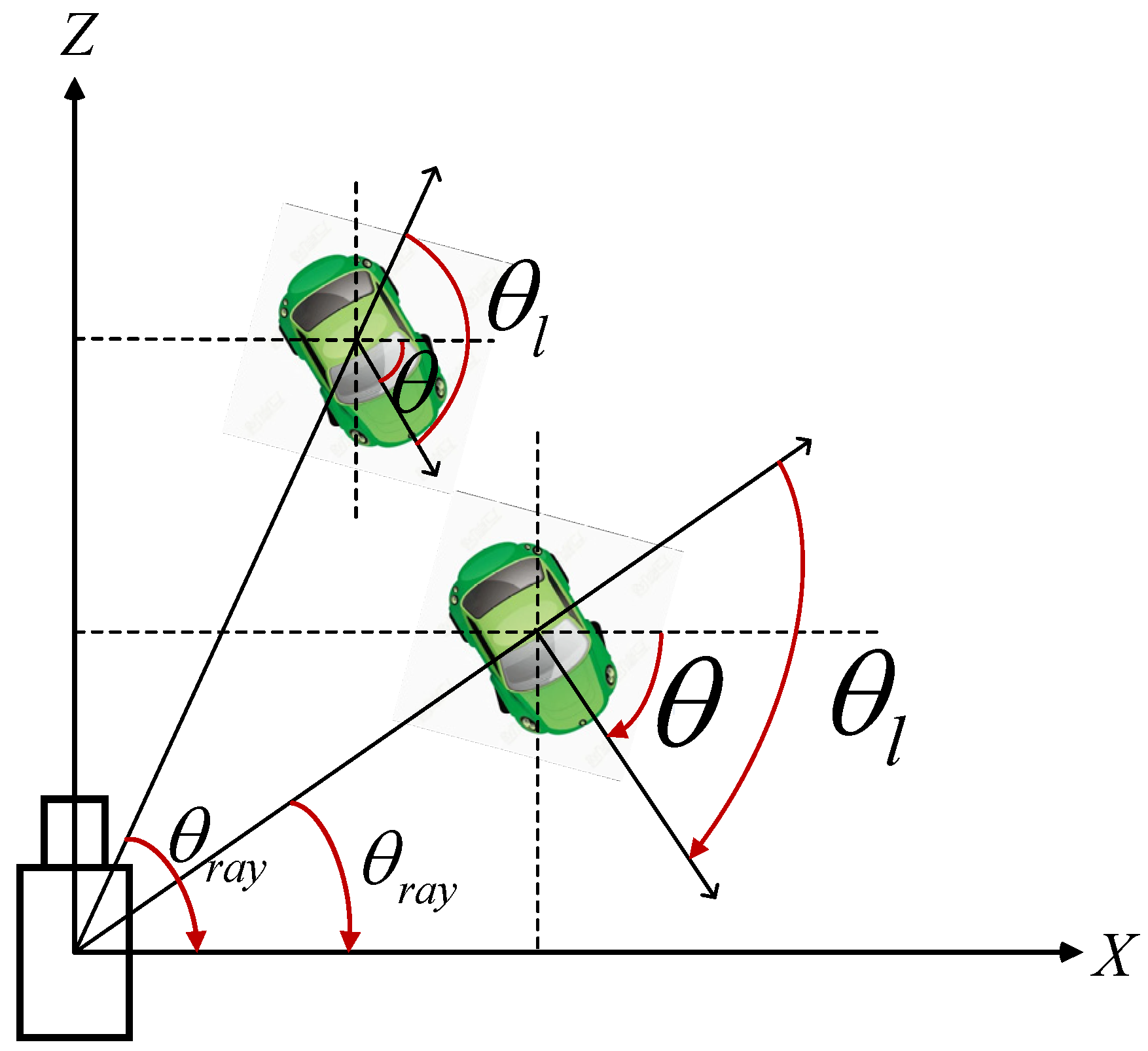
The angle detection branch estimates the heading angle of the object, which is the global angle $\theta$. As shown in Figure 6, when the car drives in a straight line, the global angle $\theta$ of the car remains unchanged, the imaging angle of the car on the image plane follows the angle ${\theta }_{ray}$ in a constant change, and the local angle ${\theta }_l$ changes accordingly. In view of the high correlation between the imaging angle of the object on the image plane and the local angle of the object, we first estimate the local angle ${\theta }_l$ and then utilize the following formula to obtain the global angle $\theta$.

$$\theta ={\theta }_l-{\theta }_{ray}={\theta }_l-\arctan \left(\frac{z}{x}\right)$$

(8)

Referring to the multi-bin regression method of Deep3Dbox [16], we estimate the local angle ${\theta }_l$ of the object by means of a multi-interval classification and residual regression.

3.1.6. Auxiliary Learning

Different from GS3D [9], Decoupled-3D [42], SMOKE [34], and other 3D object detection algorithms that only estimate the 3D parameters, our keypoint estimation network estimates not only the 3D box’s parameters but also the 2D box’s parameters. We hope to utilize the high precision of 2D object detection to aid in the learning of the 3D box’s parameters. The auxiliary learning increases the constraints of the algorithm and is conducive to the improvement of the algorithm’s precision. Refer to Faster-RCNN [43] for the implementation details of the classification and localization for 2D detection.

Loss function of the initial 3D information estimation.

The loss function of the first stage of the algorithm is as follows:

$$L_1=L_{\theta }+L_{\dim }+L_{depth}+L_{xy}+\alpha L_{2d}$$

(9)

where $L_{\theta }$ represents the local angle estimation loss, the including multi-interval classification loss and interval residual regression loss, the classification loss adopts the standard cross entropy loss function, and the residual regression loss adopts the L1 loss function; $L_{\dim }$ represents the dimension estimation loss, using the L1 loss function; and $L_{depth}$ represents the depth offset estimation loss, using the SmoothL1 loss function. $L_{xy}$ represents the position offset loss of the center point; we use the SmoothL1 loss function to perform a two-stage supervised regression on the keypoints $L_{xy}$ as follows:

$$\begin{array}{l}{L}_{xy}=smooth{L}_1\left(b_{2d}\left(x_{2d},y_{2d}\right)+\left(△x_1,△y_1\right),b_{pro}^{gt}\right)\\ +smooth{L}_1\left(b_{2d}\left(x_{2d},y_{2d}\right)+\left(△x_1,△y_1\right)+\left(△x_2,△y_2\right),b_{pro}^{gt}\right)\end{array}$$

(10)

$L_{2d}$ represents the classification loss and regression loss of the again estimated 2D box. The classification loss utilizes the cross-entropy loss function and the regression loss utilizes the SmoothL1 loss function. $\alpha =0.25$ is the loss scaling factor.

3.2. Refinement of the 3D Box

When MultiFusion [36], PatchNet [12], etc., feed the generated pseudo-lidar to the CNN in the form of the XYZ map for the feature extraction, operations such as convolution and pooling will continuously reduce the resolution of the feature map, resulting in the loss of some key information, which seriously affects the precision of the algorithm. Considering the above problems, when we feed the data fused with pseudo-lidar and image information into the CNN for the keypoint-based initial 3D box estimation, there is another data processing method of the pseudo-lidar. We project the pseudo-lidar onto the bird’s-eye view and use the bird’s-eye view features to refine the initial 3D box on the XZ plane, which compensates for the information lost in the keypoint estimation branch to a certain extent.

The method of generating a bird’s-eye view refers to AVOD [11]. We clip the pseudo-lidar to the [−40, 40] × [0, 70] range of the XZ plane to include all the points in the camera’s field of view and then divide the grid evenly in the XZ plane, finally filling each grid with the maximum height of the point clouds as the content of the grid, and a bird’s-eye view containing direct spatial information is obtained. We take the center point of the initial 3D box as the reference point, enlarge its length, width, and height to double the original box to obtain a larger 3D box, and then project the larger 3D box onto the bird’s-eye view to obtain the region bird’s-eye view, finally feeding it into a deep neural network for the information’s extraction, estimating the offsets $x,y,z,l,w,h,\theta$ of the initial 3D box. At last, these offsets and the parameters of the initial 3D box are added together to obtain a more accurate 3D box.

Compared with Decoupled-3D [42], MultiFusion [36], PatchNet [12], and other algorithms that also introduce extra depth information for detection, Decoupled-3D [42] uses the bird’s-eye view generated by the pseudo-lidar for the refinement of the initial 3D box, lacking the direct use for the pseudo-lidar stereo information. MultiFusion [36] and PatchNet [12] do not utilize the bird’s-eye view information to compensate for the lost information of the pseudo-lidar in the keypoint estimation branch. On the basis of a single image, for the first time, we gradually fuse the image, point cloud, and bird’s-eye view, three different modal data to fully extract the rich information of the original image, which achieves the goal of using the different modal information of the original image to detect and refine the 3D box.

Loss function of the refinement stage:

$$L_2=\mathrm{smooth}L1(L_{ang}+L_{\dim }+L_{poz})$$

(11)

The loss function of the refinement stage uniformly adopts a smoothL1 loss function to calculate the loss of each residual amount, where $L_{ang}$ represents the angle offset estimation loss, $L_{\dim }$ represents the dimension offset estimation loss, and $L_{poz}$ represents the position offset estimation loss.

4. Experiments

4.1. Dataset

We trained and validated our algorithm on the challenging KITTI [14] dataset, which has a total of 7481 training images and 7518 test images, because the test set lacks ground truth, and the test set’s server access is limited, so we follow the previous example and divide the training set into two parts, of which 3712 images are used for training and the remaining 3769 images are used for validation. According to the severity of the object truncation and occlusion in the KITTI dataset, we classify the objects in the KITTI dataset into three difficulty levels: easy, moderate, and difficult, as shown in Figure 7.

4.2. Experimental Details

We fuse the high score 2D region of interest and the region pseudo-lidar with attention and then feed the fused data into the keypoint estimation network for an initial 3D object detection. The input of the keypoint estimation network is scaled to 224 × 224 and then is sent to the VGG19 pre-trained on ImageNet to extract the object’s features. The resolution of the feature map of the last layer is 7 × 7 and multiple detection branches are connected behind it to estimate the 3D parameters of the 3D box and the 2D parameters of the 2D box, respectively. Each detection branch has three fully connected layers, the number of the output channels of the first two fully connected layers is 256, and the number of the output channels of the last fully connected layer is determined by the predicted parameter’s attributes. The operation of re-estimating the position and score of the 2D box belongs to auxiliary learning mainly to increase the constraints so as to estimate the parameters of the 3D box more accurately. During the training process of the keypoint regression network, the conventional data enhancement methods such as dithering, flipping, and changing the brightness or contrast are used; the optimization method is the SGD (stochastic gradient descent) algorithm, the initial learning rate is 0.0001, and the decay factor is 0.1 (every five epochs) for a total of 25 epochs of training. The network in the refinement stage is mainly a series of convolutional layers and a fully connected layer, and finally a detection head that estimates the residual amount of each 3D parameter. The computational performance of our algorithm is relatively efficient. The mean inference time of our algorithm over val1 for the initial 3D box estimation stage and the refinement stage reaches 76 ms on a single GPU. The configuration of our algorithm in the training and inference stages is Ubuntu18, a single GeForce 1080Ti GPU.

5. Experimental Results

The 3D detection and localization performance of our algorithm on KITTI is shown in

Table 1. Comparisons of and on KITTI val1/val2 sets.

Method	$\mathit{A}{\mathit{P}}_{3\mathit{d}}$			$\mathit{A}{\mathit{P}}_{\mathit{b}\mathit{e}\mathit{v}}$
	Easy	Moderate	Hard	Easy	Moderate	Hard
MultiFusion [36]	10.53/7.85	5.69/5.39	5.39/4.73	22.03/19.20	13.63/12.17	11.60/10.89
ROI-10D [32]	-/9.61	-/6.63	-/6.29	-/14.50	-/9.91	-/8.73
MonoPair [44]	-/16.28	-/12.30	-/10.42	-/24.12	-/18.17	-/15.76
SMOKE [34]	-/14.76	-/12.85	-/11.50	-/19.99	-/15.61	-/15.28
RTM-3D [8]	19.47/20.77	16.29/16.86	15.27/16.63	24.74/25.56	22.03/22.12	18.05/20.91
Pseudo-Lidar [19]	-/19.50	-/17.20	-/16.20	-	-	-
UR3D [45]	26.30/28.05	16.75/18.76	13.60/16.55	36.15/37.35	25.25/26.01	20.12/20.84
Lite-FPN [31]	-/18.01	-/15.29	-/14.28	-/24.83	-/20.50	-/17.65
D4LCN [18]	24.29/26.97	19.54/21.71	16.38/18.22	-/34.82	-/25.83	-/23.53
AM3D [17]	-/32.23	-/21.09	-/17.26	-/43.75	-/28.39	-/23.87
PatchNet [12]	-/35.1	-/22.0	-/19.6	-/44.4	-/29.1	-/24.1
Ours	31.61/34.85	21.67/22.59	18.76/19.81	43.84/44.71	29.66/30.67	24.78/25.05

.

5.1. Compared to Other Algorithms

We compare our approach with monocular state-of-the-art methods on the KITTI benchmark, including ROI-10D [32], MonoPair [44], M3D-RPN [30], UR3D [45], SMOKE [34], Lite-FPN [31], RTM3D [8], Pseudo-Lidar [19], D4LCN [18], AM3D [17], and PatchNet [12]. The judging criterion is to compare the average precision of the 3D detection and the location. $A{P}_{3d}$ reflects the accuracy of the position estimation of the object in 3D space. $A{P}_{bev}$ reflects the accuracy of the location of the object on the bird’s-eye view.

5.2. Validation Set Comparison Results

Following the precedent, we conduct 3D object detection experiments and localization experiments for both dataset segmentation methods; the experimental results are shown in Table 1. ROI-10D [32] superimposes the depth map and image’s features and directly estimates the 3D box on the basis of 2D detection; the precision of the algorithm strongly depends on the accuracy of the 2D object detection. In comparison, our method performs initial coarse 3D object detection on the basis of 2D detection and utilize the bird’s-eye view feature generated by the pseudo-lidar to refine the initial 3D box; Pseudo-Lidar [19] converts the depth map to pseudo-lidar and feeds it to a lidar-based 3D detection framework to accomplish the 3D object detection. As a contrast, our method performs an information extraction and application for the generated pseudo-lidar in two different data modalities.

5.3. Test Set Comparison Results

Our experimental results on the KITTI test dataset are shown in

Table 2. Comparisons of and on KITTI test sets.

Method	$\mathit{A}{\mathit{P}}_{3\mathit{d}}$			$\mathit{A}{\mathit{P}}_{\mathit{b}\mathit{e}\mathit{v}}$
	Easy	Moderate	Hard	Easy	Moderate	Hard
ROI-10D [32]	4.32	2.02	1.46	9.78	4.91	3.74
MultiFusion [36]	7.08	5.18	4.68	13.73	9.62	8.22
UR3D [45]	15.58	8.61	6.00	21.85	12.51	9.20
RTM-3D [8]	14.41	10.34	8.77	-	-	-
MonoPair [44]	13.04	9.99	8.65	19.28	14.83	12.89
SMOKE [34]	14.03	9.76	7.84	20.83	14.49	12.75
D4LCN [18]	16.65	11.72	9.51	-	-	-
Lite-FPN [31]	15.32	10.64	8.59	26.67	17.58	14.51
AM3D [17]	16.50	10.74	9.52	-	-	-
PatchNet [12]	15.68	11.12	10.17	-	-	-
Ours	15.86	11.41	10.08	28.79	18.61	15.27

. D4LCN [18] uses the depth-guided convolution generated by the depth map to extract the image’s features for directly estimating the 3D object box; operations such as convolution and pooling in the process of the features’ extraction will result in losing some detailed information. In comparison, we extract and learn the features in three different modal forms on the original image, which extracts the information of the original image more comprehensively and accurately and also makes up for the lost information in the keypoint branch to a certain extent. At the same time, it is worth noting that compared with the validation set’s experimental performance, the test set’s experimental performance has declined because the data used in the training of the depth estimator overlap with the data used in our algorithm training, which has a data overfitting problem. It is a common problem for a class of algorithms that utilize a depth estimator to provide extra depth information, for instance, ROI-10D [32] also suffers from the same problem.

5.4. Performance Difference of Three Depth Estimators

In

Table 3. Performance difference of three depth estimators.

Method	$\mathit{A}{\mathit{P}}_{3\mathit{d}}$			$\mathit{A}{\mathit{P}}_{\mathit{b}\mathit{e}\mathit{v}}$
	Easy	Moderate	Hard	Easy	Moderate	Hard
MonoDepth	22.03	17.41	13.39	26.28	23.25	19.73
DORN	34.85	22.59	19.81	44.71	30.67	25.05
PSMNet	39.63	25.23	21.58	54.7	35.92	29.17

, we show the difference in the experimental performance caused by different depth estimators from MonoDepth [46], DORN [40], and PSMNet [47]. As the depth estimation accuracy improves, so does the accuracy of our algorithm.

5.5. Ablation Experiments

In this section, the effectiveness of some important structures and parameters is shown; all experiments are performed on the KITTI validation set.

5.6. Effectiveness of the Twice 3D Detection

Our method is a multi-stage 3D object detection algorithm on the basis of 2D detection. First of all, we perform 2D object detection to obtain the region of interest, estimate the initial 3D box on the feature map generated from the fusion data, and finally use the bird’s-eye view to refine the initial 3D box. We set up three groups of experiments to verify the effectiveness of the 3D box regression performed twice. In the first group, we directly estimate the 3D box’s parameters while performing the 2D detection. In the second group, on the basis of the 2D detection, we feed the fusion data of the 2D region of interest and the pseudo-lidar to the keypoint estimation network for the initial 3D object detection. In the third group, on the basis of the second group, we utilize the bird’s-eye view to refine the coarse initial 3D box to obtain a more accurate 3D box. All the experimental results are shown in

Table 4. Ablation study of 3D object regression.

Method	$\mathit{A}{\mathit{P}}_{3\mathit{d}}$			$\mathit{A}{\mathit{P}}_{\mathbf{bev}}$
	Easy	Moderate	Hard	Easy	Moderate	Hard
2D-based regression	0.41	1.34	1.2	0.73	1.82	1.95
+ keypoint-based regression	24.39	18.17	17.62	33.91	24.15	21.86
+ bird’s-eye-based regression	34.85	22.59	19.81	44.71	30.67	25.05

.

5.7. Effectiveness of Auxiliary Learning

Our algorithm performs a second 2D object detection while estimating the initial 3D box; this is to add constraints to the loss function, aiding in the learning of 3D parameters by virtue of the high precision of the 2D detection. The algorithm uses $\alpha$ to adjust the proportion of the 2D detection loss to the total loss function. In order to verify the effectiveness of the auxiliary learning, a set of ablation experiments is set up. The experimental results are shown in

Table 5. Ablation study of auxiliary learning.

Method	$\mathit{A}{\mathit{P}}_{3\mathit{d}}$			$\mathit{A}{\mathit{P}}_{\mathbf{bev}}$
	Easy	Moderate	Hard	Easy	Moderate	Hard
$\alpha =0$	31.89	21.09	19.16	39.75	27.83	24.12
$\alpha =0.1$	34.27	21.96	19.65	43.54	29.86	24.76
$\alpha =0.2$	34.65	22.32	19.77	44.16	30.35	24.97
$\alpha =0.25$	34.85	22.59	19.81	44.71	30.67	25.05
$\alpha =0.3$	34.54	22.29	19.68	44.47	30.24	24.70

.

5.8. Ablation Experiment of Offsets Estimation

When estimating the initial 3D box, our algorithm estimates the offsets of the keypoints of the 3D box relative to the center point of the 2D box twice, which can increase the constraints of the loss function and improve the precision of the initial 3D object detection. The results of the ablation experiments are shown in

Table 6. Ablation study of offsets.

Method	$\mathit{A}{\mathit{P}}_{3\mathit{d}}$			$\mathit{A}{\mathit{P}}_{\mathbf{bev}}$
	Easy	Moderate	Hard	Easy	Moderate	Hard
$offset=(△x_1,△y_2)$	33.27	21.89	19.54	42.91	29.83	24.86
$offset=(△x_1,△y_1)+(△x_2,△y_2)$	34.85	22.59	19.81	44.71	30.67	25.05

.

5.9. Ablation Experiment of Attention Mechanism

For the information fusion method of the image modality and attentional pseudo-lidar modality, the following three groups of ablation experiments were carried out. In the first group, the two-modal information is fused directly without an attention mechanism. In the second group, after the region pseudo-lidar is multiplied by the attention map generated by the region pseudo-lidar, it is fused with the image information for the 3D object detection. In the third group, after the pseudo-lidar is multiplied by the attention map generated by the image region, it is fused with the image information for the 3D object detection. The experimental results are shown in

Table 7. Ablation study of attention mechanism.

Method	$\mathit{A}{\mathit{P}}_{3\mathit{d}}$			$\mathit{A}{\mathit{P}}_{\mathbf{bev}}$
	Easy	Moderate	Hard	Easy	Moderate	Hard
(1) Without attention	22.27	18.35	16.54	29.81	23.65	20.86
(2) Image-based attention	27.32	20.95	18.73	36.39	27.75	23.45
(3) Point cloud-based attention	34.85	22.59	19.81	44.71	30.67	25.05

. It can be seen from the table that the experimental performance of the first group directly fusing the two-modality data is the worst, and the experimental performance of the third group using the attention map generated by image region for object detection is the best because the image region is more accurate than the region pseudo-lidar, so the attention map generated by the former is also more accurate and the experimental performance is better.

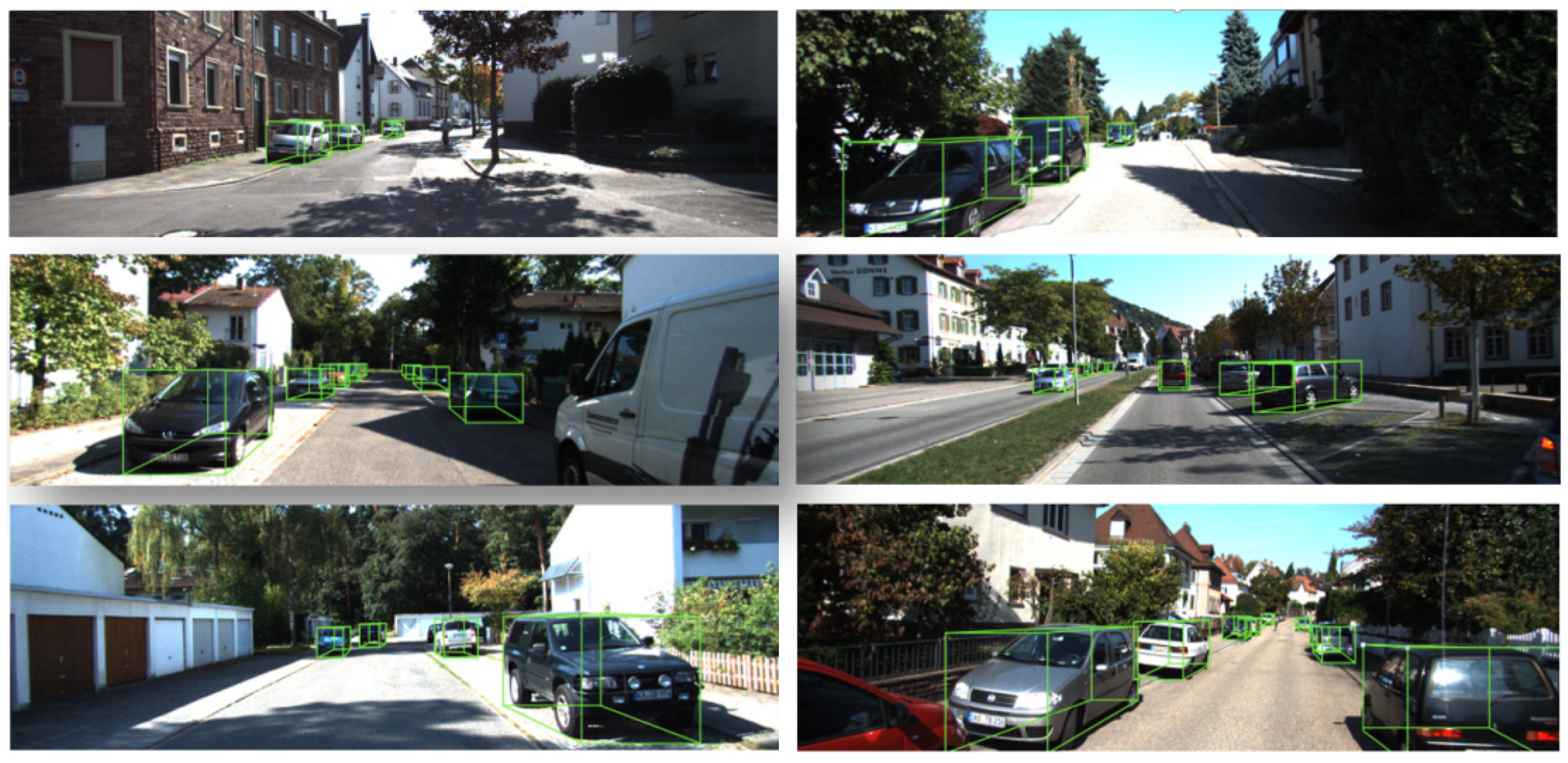
5.10. Qualitative Experimental Results

This section presents the qualitative experimental results of our method on the KITTI dataset, as shown in Figure 8. Most of the objects are well detected by our algorithm, which verifies the effectiveness of our method. At the same time, it is worth noting that some objects are missed or false positives appear due to reasons such as occlusion, truncation, and background clutter. Some objects are missed or the position estimation is inaccurate because they are far away from the camera. Solving these problems is the future optimization direction of our algorithm.

6. Conclusions

In this paper, we propose a monocular 3D object detection algorithm based on pseudo-multimodal information extraction and keypoint estimation, which fuse the conventional data processing approaches of three different data modalities for 3D object detection. The image’s features fused with the region pseudo-lidar information are easier to learn the accurate position of the object than the original image features. The operation of fusing the bird’s-eye view modal information compensates for the information lost in the keypoint branch to a certain extent, which makes the precision of the 3D object detection further improved. The fusion processing of three different modal information enables our algorithm to extract the image information and fuse the image’s features in multiple dimensions, which greatly improves the precision of current monocular 3D object detection algorithms and achieves a state-of-the-art experimental performance of the same category of algorithm.

References

- Lang, A.H.; Vora, S.; Caesar, H.; Zhou, L.; Yang, J.; Beijbom, O. PointPillars: Fast encoders for object detection from point clouds. In Proceedings of the IEEE/CVF International Conference on Computer Vision, Seoul, Korea, 27 October–2 November 2019. [Google Scholar]
- Zhang, Y.; Hu, Q.; Xu, G.; Ma, Y.; Wan, J.; Guo, Y. Not All Points Are Equal: Learning Highly Efficient Point-based Detectors for 3D LiDAR Point Clouds. In Proceedings of the IEEE/CVF International Conference on Computer Vision, New Orleans, LA, USA, 18–24 June 2022. [Google Scholar]
- Shi, S.; Wang, X.; Li, H. PointRCNN: 3d object proposal generation and detection from point cloud. In Proceedings of the IEEE/CVF International Conference on Computer Vision, Seoul, Korea, 27 October–2 November 2019. [Google Scholar]
- Chen, Y.; Liu, S.; Shen, X.; Jia, J. DSGN: Deep Stereo Geometry Network for 3D Object Detection. In Proceedings of the IEEE/CVF Conference on Computer Vision and Pattern Recognition, Seattle, WA, USA, 13–19 June 2020. [Google Scholar]
- Li, P.; Chen, X.; Shen, S. Stereo R-CNN based 3d object detection for autonomous driving. In Proceedings of the IEEE/CVF International Conference on Computer Vision, Seoul, Korea, 27 October–2 November 2019. [Google Scholar]
- Pon, A.D.; Ku, J.; Li, C.; Waslander, S.L. Object-Centric Stereo Matching for 3D Object Detection. In Proceedings of the 2020 IEEE International Conference on Robotics and Automation (ICRA), online, 31 May–31 August 2020. [Google Scholar]
- Ku, J.; Pon, A.D.; Waslander, S.L. Monocular 3d object detection leveraging accurate proposals and shape reconstruction. In Proceedings of the IEEE/CVF International Conference on Computer Vision, Seoul, Korea, 27 October–2 November 2019. [Google Scholar]
- Li, P.; Zhao, H.; Liu, P.; Cao, F. RTM3D: Real-time monocular 3d detection from object keypoints for autonomous driving. In Proceedings of the European Conference on Computer Vision, Glasgow, UK, 23–28 August 2020. [Google Scholar]
- Li, B.; Ouyang, W.; Sheng, L.; Zeng, X.; Wang, X. GS3D: An efficient 3d object detection framework for autonomous driving. In Proceedings of the IEEE/CVF International Conference on Computer Vision, Seoul, Korea, 27 October–2 November 2019. [Google Scholar]
- Weng, X.; Kitani, K. Monocular 3D Object Detection with Pseudo-LiDAR Point Cloud. In Proceedings of the IEEE/CVF International Conference on Computer Vision, Seoul, Korea, 27 October–2 November 2019. [Google Scholar]
- Ku, J.; Mozifian, M.; Lee, J.; Harakeh, A.; Waslander, S.L. Joint 3D Proposal Generation and Object Detection from View Aggregation. In Proceedings of the IEEE/CVF International Conference on Computer Vision, Salt Lake City, UT, USA, 18–23 June 2018. [Google Scholar]
- Ma, X.; Liu, S.; Xia, Z.; Zhang, H.; Zeng, X.; Ouyang, W. Rethinking Pseudo-LiDAR Representation. In Proceedings of the European Conference on Computer Vision, Glasgow, UK, 23–28 August 2020. [Google Scholar]
- Chen, X.; Ma, H.; Wan, J.; Li, B.; Xia, T. Multi-View 3D Object Detection Network for Autonomous Driving. In Proceedings of the IEEE/CVF International Conference on Computer Vision, Venice, Italy, 22–29 October 2017. [Google Scholar]
- Geiger, A.; Lenz, P.; Urtasun, R. Are we ready for autonomous driving? the kitti vision benchmark suite. In Proceedings of the IEEE/CVF International Conference on Computer Vision, Providence, RI, USA, 17 October 2012. [Google Scholar]
- Liu, L.; Lu, J.; Xu, C.; Tian, Q.; Zhou, J. Deep fitting degree scoring network for monocular 3d object detection. In Proceedings of the IEEE/CVF International Conference on Computer Vision, Seoul, Korea, 27 October–2 November 2019. [Google Scholar]
- Mousavian, A.; Anguelov, D.; Flynn, J.; Kosecka, J. 3D bounding box estimation using deep learning and geometry. In Proceedings of the IEEE/CVF International Conference on Computer Vision, Venice, Italy, 22–29 October 2017. [Google Scholar]
- Ma, X.; Wang, Z.; Li, H.; Ouyang, W.; Pengbo, Z. Accurate monocular 3d object detection via color-embedded 3d reconstruction for autonomous driving. In Proceedings of the IEEE/CVF International Conference on Computer Vision, Seoul, Korea, 27 October–2 November 2019. [Google Scholar]
- Ding, M.; Yi, H.; Wang, Z.; Shi, J.; Lu, Z.; Luo, P. Learning Depth-Guided Convolutions for Monocular 3D Object Detection. In Proceedings of the IEEE/CVF International Conference on Computer Vision, Seattle, WA, USA, 13–19 June 2020. [Google Scholar]
- Wang, Y.; Chao, W.; Garg, D.; Hariharan, B.; Campbell, M.; Weinberger, K. Pseudo-LiDAR from Visual Depth Estimation: Bridging the Gap in 3D Object Detection for Autonomous Driving. In Proceedings of the IEEE/CVF International Conference on Computer Vision, Seoul, Korea, 27 October–2 November 2019. [Google Scholar]
- Zhou, Y.; Tuzel, O. VoxelNet: End-to-end learning for point cloud based 3d object detection. In Proceedings of the IEEE/CVF International Conference on Computer Vision, Salt Lake City, UT, USA, 18–23 June 2018. [Google Scholar]
- Yan, Y.; Mao, Y.; Li, B. Second: Sparsely embedded convolutional detection. Sensors 2018, 18, 3337. [Google Scholar] [CrossRef] [PubMed]
- Yang, B.; Luo, W.; Urtasun, R. Pixor: Realtime 3d object detection from point clouds. In Proceedings of the IEEE/CVF International Conference on Computer Vision, Salt Lake City, UT, USA, 18–23 June 2018. [Google Scholar]
- Chen, Y.; Liu, S.; Shen, X.; Jia, J. Fast-Point-RCNN. In Proceedings of the IEEE/CVF International Conference on Computer Vision, Seoul, Korea, 27 October–2 November 2019. [Google Scholar]
- Wang, Y.; Yang, B.; Hu, R.; Liang, M.; Urtasun, R. PLUMENet: Efficient 3D Object Detection from Stereo Images. In Proceedings of the IEEE/RSJ International Conference on Intelligent Robots and Systems, Prague, Czech Republic, 27 September–1 October 2021. [Google Scholar]
- You, Y.; Wang, Y.; Chao, W.-L.; Garg, D.; Pleiss, G.; Hariharan, B.; Campbell, M.; Weinberger, K.Q. Pseudo-LiDAR++: Accurate Depth for 3D Object Detection in Autonomous Driving. arXiv 2019, arXiv:1906.06310v1. [Google Scholar]
- Peng, W.; Pan, H.; Liu, H.; Sun, Y. IDA-3D: Instance-Depth-Aware 3D Object Detection from Stereo Vision for Autonomous Driving. In Proceedings of the IEEE/CVF International Conference on Computer Vision, Seattle, WA, USA, 13–19 June 2020. [Google Scholar]
- Guo, X.; Shi, S.; Wang, X.; Li, H. LIGA-Stereo: Learning LiDAR Geometry Aware Representations for Stereo-based 3D Detector. In Proceedings of the IEEE/CVF International Conference on Computer Vision, Montreal, BC, Canada, 11–17 October 2021. [Google Scholar]
- Sun, J.; Chen, L.; Xie, Y.; Zhang, S.; Jiang, Q.; Zhou, X.; Bao, H. Disp R-CNN: Stereo 3D Object Detection via Shape Prior Guided Instance Disparity Estimation. In Proceedings of the IEEE/CVF Conference on Computer Vision and Pattern Recognition, Seattle, WA, USA, 13–19 June 2020. [Google Scholar]
- Liu, Y.; Wang, L.; Liu, M. y YOLOStereo3D: A Step Back to 2D for Efficient Stereo 3D Detection. In Proceedings of the 2021 IEEE International Conference on Robotics and Automation (ICRA), Xi’an, China, 30 May–5 June 2021. [Google Scholar]
- Brazil, G.; Liu, X. M3D-RPN: Monocular 3d region proposal network for object detection. In Proceedings of the IEEE/CVF International Conference on Computer Vision, Seoul, Korea, 27 October–2 November 2019. [Google Scholar]
- Yang, L.; Zhang, X.; Wang, L.; Zhu, M.; Li, J. Lite-FPN for Keypoint-based Monocular 3D Object Detection. arXiv 2021, arXiv:2105.00268v2. [Google Scholar]
- Manhardt, F.; Kehl, W.; Gaidon, A. ROI-10D: Monocular lifting of 2d detection to 6d pose and metric shape. In Proceedings of the IEEE/CVF International Conference on Computer Vision, Seoul, Korea, 27 October–2 November 2019. [Google Scholar]
- Liu, X.; Xue, N.; Wu, T. Learning Auxiliary Monocular Contexts Helps Monocular 3D Object Detection. In Proceedings of the AAAI Conference on Artificial Intelligence, Virtually, 22 February–1 March 2022. [Google Scholar]
- Liu, Z.; Wu, Z.; Toth, R. SMOKE: Single-stage monocular 3d object detection via keypoint estimation. In Proceedings of the IEEE/CVF International Conference on Computer Vision, Seattle, WA, USA, 13–19 June 2020. [Google Scholar]
- Zhou, X.; Wang, D.; Krahenbuhl, P. Objects as points. arXiv 2019, arXiv:1904.07850. [Google Scholar]
- Xu, B.; Chen, Z. Multi-level fusion based 3D object detection from monocular images. In Proceedings of the IEEE/CVF International Conference on Computer Vision, Salt Lake City, UT, USA, 18–23 June 2018. [Google Scholar]
- Reading, C.; Harakeh, A.; Chae, J. Categorical Depth Distribution Network for Monocular 3D Object Detection. In Proceedings of the IEEE/CVF International Conference on Computer Vision, Montreal, BC, Canada, 11–17 October 2021. [Google Scholar]
- Gupta, I.; Rangesh, A.; Trivedi, M. 3D Bounding Boxes for Road Vehicles: A One-Stage, Localization Prioritized Approach using Single Monocular Images. In Proceedings of the European Conference on Computer Vision, Munich, Germany, 8–14 September 2018. [Google Scholar]
- Cai, Z.; Fan, Q.; Feris, R.S.; Vasconcelos, N. A Unified Multi-scale Deep Convolutional Neural Network for Fast Object Detection. In Proceedings of the European Conference on Computer Vision, Amsterdam, The Netherlands, 11–14 October 2016. [Google Scholar]
- Fu, H.; Gong, M.; Wang, C.; Batmanghelich, K.; Tao, D. Deep Ordinal Regression Network for Monocular Depth Estimation. In Proceedings of the IEEE/CVF International Conference on Computer Vision, Salt Lake City, UT, USA, 18–23 June 2018. [Google Scholar]
- Qi, C.R.; Liu, W.; Wu, C.; Su, H.; Guibas, L.J. Frustum pointnets for 3d object detection from RGB-D data. In Proceedings of the IEEE/CVF International Conference on Computer Vision, Salt Lake City, UT, USA, 18–23 June 2018. [Google Scholar]
- Cai, Y.; Li, B.; Jiao, Z.; Li, H.; Zeng, X.; Wang, X. Monocular 3d object detection with decoupled structured polygon estimation and height-guided depth estimation. In Proceedings of the AAAI Conference on Artificial Intelligence, New York, NY, USA, 7–12 February 2020. [Google Scholar]
- Ren, S.; He, K.; Girshick, R.; Sun, J. Faster R-CNN: Towards real-time object detection with region proposal networks. arXiv 2015, arXiv:1506.01497. [Google Scholar] [CrossRef] [PubMed]
- Chen, Y.; Tai, L.; Sun, K.; Li, M. MonoPair: Monocular 3D Object Detection Using Pairwise Spatial Relationships. In Proceedings of the IEEE/CVF International Conference on Computer Vision, Seattle, WA, USA, 13–19 June 2020. [Google Scholar]
- Shi, X.; Chen, Z.; Kim, T.-K. Distance-Normalized Unified Representation for Monocular 3D Object Detection. In Proceedings of the European Conference on Computer Vision, Glasgow, UK, 23–28 August 2020. [Google Scholar]
- Godard, C.; Aodha, O.M.; Brostow, G.J. Unsupervised monocular depth estimation with left-right consistency. In Proceedings of the IEEE/CVF International Conference on Computer Vision, Venice, Italy, 22–29 October 2017. [Google Scholar]
- Chang, J.-R.; Chen, Y.-S. Pyramid stereo matching network. In Proceedings of the IEEE/CVF International Conference on Computer Vision, Salt Lake City, UT, USA, 18–23 June 2018. [Google Scholar]
Figure 1.
Architecture of our proposed method. Considering the lack of depth information of the monocular image, we fuse the pseudo point cloud information and image information to perform keypoint-based initial 3D object estimation. In order to make up for the information losing due to the convolution or pooling in the initial estimation stage, we refine the initial 3D box in the XZ plane using the bird’s-eye view generated from the pseudo-point cloud.
Figure 2.
Pseudo-multimodal data used for fusion in our algorithm. From left to right, there are image patches, the corresponding region pseudo-lidar point cloud, and the corresponding panoramic bird’s-eye view. The area surrounded by the red box in the bird’s-eye view is where the object is located.
Figure 3.
Information fusion process with attention mechanism of 2D region of interest and region pseudo-lidar.
Figure 4.
Difference between the projected point of the center point of the 3D box and the center point of the 2D box.
Figure 5.
Detection head branches of the keypoint estimation network.
Figure 6.
Difference between the global angle and the local angle . is the angle between the ray from the center of the camera to the object and the X-axis of the camera, determining the imaging angle of the object on the image plane.
Figure 7.
Different difficulty levels of samples. The objects pointed by the yellow arrows belong to the “Easy” difficulty category, which are mostly unoccluded or untruncated, and relatively close to the camera; the objects pointed by the blue arrows belong to the “Moderate” difficulty category, which are slightly occluded or truncated, or slightly farther away from the camera. The objects pointed by the red arrows belong to the “Hard” difficulty category, which are severely occluded or truncated, or far away from the camera.
Figure 8.
Qualitative experimental results of our method.