Article

Design of Robust Sensing Matrix for UAV Images Encryption and Compression

1
The College of Information Engineering, Zhejiang University of Technology, Hangzhou 310023, China
2
The School of Information Science and Technology, Hangzhou Normal University, Hangzhou 311121, China
*
Author to whom correspondence should be addressed.
Appl. Sci. 2023, 13(3), 1575; https://doi.org/10.3390/app13031575
Submission received: 17 November 2022 / Revised: 28 December 2022 / Accepted: 21 January 2023 / Published: 26 January 2023
(This article belongs to the Special Issue New Technology for Autonomous UAV Monitoring)

Abstract

:
The sparse representation error (SRE) exists when the images are represented sparsely. The SRE is particularly large in unmanned aerial vehicles (UAV) images due to the disturbance of the harsh environment or the instability of its flight, which will bring more noise. In the compressed sensing (CS) system, the projected SRE in the compressed measurement will bring a significant challenge to the recovery accuracy of the images. In this work, a new SRE structure is proposed. Following the new structure, a lower sparse representation error (LSRE) is achieved by eliminating groups of sparse representation. With the proposed LSRE modeling, a robust sensing matrix is designed to compress and encrypt the UAV images. Experiments for UAV images are carried out to compare the recovery performance of the proposed algorithm with the existing related algorithms. The results of the proposed algorithm reveal superior recovery accuracy. The new CS framework with the proposed sensing matrix to address the scenario of UAV images with large SRE is dominant.

1. Introduction

Unmanned aerial vehicles (UAV) [1,2,3] mainly orient to low-altitude remote sensing, which has advantages in complex scenarios exploration. Compared to manual detection, UAV can reach the place where a ground search is difficult to approach by controlling the flight attitude [4,5]. Hence, adopting a UAV to capture images can reduce costs and increase flexibility. Improving the transmission security and efficiency of captured images from UAV has become our concern. The compressed sensing (CS) technique [6,7,8] can compress and encrypt UAV images simultaneously to achieve a low-dimensional matrix. The low-dimensional matrix can be transmitted safely and efficiently due to its incomprehensible meaning. At the decoding stage, the low-dimensional matrix can be recovered with high accuracy by employing the CS technique. In our paper, how to design a robust compressed sensing framework to deal with the large SRE in the UAV images is the main focus of our research.
CS technique [9,10,11,12,13] projects compressible data x N × 1 into low dimensional measurements y M × 1 by adopting the sensing matrix Φ M × N , which can be expressed as:
y = Φ x .
Equation (1) describes the process for data compression and encryption by using the sensing matrix Φ M × N . As  M N , it is an underdetermined problem that has infinite solutions. The constraint of sparseness can be added to the data x , and its form of sparse representation can be written as:
x = l = 1 L α ( l ) Ψ ( : , l ) = Ψ α ,
in which the matrix Ψ N × L is named dictionary with its column atoms { Ψ ( : , l ) } l = 1 L , and the α ( l ) is the lth element of the sparse coefficient α L × 1 . Then, the vector x is said K-sparse in Ψ if the sparse coefficient α satisfying α 0 K . · 0 denotes the number of non-zero elements.
Following the data x in (1) being substituted with (2), the mathematical framework of CS is concluded as:
y = Φ Ψ α D α ,
in which the matrix D M × L is the so-called equivalent dictionary. Under the sparsity condition on x , a unique mapping between the measurement y and the original data x  [14,15] is established. Hence, with the given sensing matrix Φ and dictionary Ψ , the process of decryption and recovery can be executed as:
α ^ = arg min α α 0 s . t . y = D α .
the estimate α ^ is achieved by solving the above problem. The greedy algorithms deal with the above optimization problem of 0 -norm constraint, such as Orthogonal Matching Pursuit (OMP) [16]. When the constraint in (4) becomes 1 -norm, it is solved by employing Basis Pursuit (BP) [17] and a Least Absolute Shrinkage and Selection Operator (LASSO) [18]. Then, the estimated data x ^ is recovered via calculating x ^ = Ψ α ^ .
In order to improve the recovery performance, some optimal regulations are proposed to obtain a better property for the equivalent dictionary, such as mutual coherence [19,20,21] and the averaged mutual coherence denoted as μ a v ( D ) [22]. While mutual coherence demonstrates the worst case for successful recovery, it does not emphasize the actual performance for the recovery precise. Hence, the author in [22] proposed the averaged mutual coherence to play better behavior.
Based on this effective design criteria, some algorithms [23,24,25] are proposed to optimize the sensing matrix by minimizing the following cost function when the dictionary is given:
min Φ , G t G t G F 2 s . t . G = Ψ T Φ T Φ Ψ ,
where · F denotes the Frobenius-norm. G L × L is the Gram of the equivalent dictionary (denoted as G = D T D ). G t L × L is defined as a target Gram. The physical meaning is that the off-diagonal elements in G represent the coherence between any atoms in equivalent dictionary, and approaching each value of the off-diagonal elements to the certain value of the target Gram, which results in the minimization of the averaged mutual coherence. Hence, minimizing μ a v ( D ) is the goal that we design the sensing matrix.
The selection of target gram will influence the performance of data recovery. The tight frame (TF)-based matrix [26,27] can provide better performance for the absolute sparse data. Besides, the references in [23,24,25] also elaborate that selecting the identity matrix as the target Gram can help recover image data better than the tight frame (TF)-based matrix ones. It is because the image data is not absolutely sparse that exists the sparse representation error. Therefore, the sparse representation for image data can be expressed as:
X = Ψ A + E ,
in which X N × Q is the given image data, and  A L × Q is its corresponding sparse matrix in dictionary Ψ N × L . E N × Q is defined as the sparse representation error (SRE). Since the SRE can not be ignored in the image data, some research [28,29,30,31] has focused on how the SRE impact the model of sensing matrix design. The general model can be expressed as:
min Φ I L G F 2 + λ Φ E F 2 ,
where I L is the target Gram G t that denotes the identity matrix with dimension L. G L × L is the Gram of the equivalent dictionary (denoted as G = D T D ). The idea in [28] indicates that the averaged mutual coherence should be minimized by the first term of the above cost function. As for the second term, the energy for SRE projected by the sensing matrix should also be minimized. For further analysis, an inappropriate sensing matrix will magnify the SRE itself, which leads to a significant error in the measurement, which will bring big challenges to the recovery accuracy of the image. Therefore, it is essential to consider the influence of SRE when the sensing matrix is designed.
Observing Equation (6), the SRE is strongly associated with sparse representation. By considering the sparse representation error (SRE) with a new model, we are able to eliminate parts of the error, and hence achieve a lower sparse representation error (LSRE). A cost function is then designed for the proposed model, in which a robust sensing matrix can be obtained by simultaneously reducing the energy of projected LSRE and averaged mutual coherence. The above-designed sensing matrix can address the images with large SRE. For example, the UAV images contain large SRE due to the disturbance of the harsh environment or the instability of its flight [32,33]. Hence, the new CS framework with the proposed sensing matrix to cope with the scenario of UAV images is dominant, which can achieve better recovery performance.
The main contributions are summarized as follows:
  • A new structure where the SRE is reduced by eliminating groups of sparse representation is proposed, which is denoted as NSSRE. The SRE is decreased to LSRE so that the excessive error is effectively controlled when being projected into measurements.
  • By employing LSRE to minimize the projected Energy, a more robust Sensing Matrix named LESM is designed to build an optimal CS system.
  • The new CS framework with the robust sensing matrix LESM is established to compress and encrypt the UAV images to improve the security and the transmission speed, which can confront the SRE in the image and lead to more accuracy of image recovery.
The rest of the paper is arranged as follows. Section 2 introduces the preliminary knowledge and related algorithms of sensing matrix design. In Section 3, the new structure to build lower SRE, and the proposed LESM algorithm for sensing matrix design is detailed. The flow chart and the procedure of the proposed CS framework are also concluded in this section. The experiments on UAV images are carried out to test the recovery performance of the proposed sensing matrix in Section 4. Section 5 makes the conclusion of this paper.

2. Preliminaries

To ensure that the sparse coefficient is recovered successfully, the regulation of mutual coherence [19,20,21] is taken into account when the equivalent dictionary is given, that is:
μ ( D ) max 1 i j L | ( D ( : , i ) ) T D ( : , j ) | D ( : , i ) 2 D ( : , j ) 2 ,
where T denotes the transpose operator. Mutual coherence is defined to calculate the worst coherence between any two atoms of D . However, the relations between mutual coherence and the sparsity K will influence whether the decryption and recovery are successful or not. The author in [19] indicates that the sparse coefficient α can be recovered exactly via (4) as long as
S   <   1 2 1 + 1 μ ( D ) .
The Equation (9) inspires us to reduce the mutual coherence of D by optimizing the sensing matrix when the dictionary is given, so that the sparsity K can achieve a larger value space. While mutual coherence provides the worst case for successful recovery, it does not emphasize the actual performance for precise recovery. Hence, the authors in [22] proposed the averaged mutual coherence to play better behavior. The definition of averaged mutual coherence can be written as:  
μ a v ( D ) ( i , j ) S a v | G ¯ ( i , j ) | N a v ,
where G ¯ is the Gram matrix of the column-normalized equivalent dictionary D and the off-diagonal elements G ¯ ( i , j ) means the coherence of D . S a v is a set that is defined as S a v = { ( i , j ) : μ ¯ | G ¯ ( i , j ) | < 1 , i j } with 0 μ ¯ < 1 . The low bound of μ ¯ is L M M ( L 1 )  [22]. N a v counts the number of elements in set S a v .
Based on above regulations for sensing matrix design, the work in [24] proposed the cost function for optimizing sensing matrix, which can be expressed as:
Φ L Z Y = arg min Φ I L G F 2 s . t . G = Ψ T Φ T Φ Ψ .
The above problem can be decomposed into two parts:
I L G F 2 = l = 1 L | 1 G ( l , l ) | 2 + i j | G ( i , j ) | 2 .
Observing the above equation, the physical meaning of the first term is to set the constraint that the columns of the dictionary approach to be normalized. The second term measures the average mutual coherence with high bound L ( L 1 ) . Hence, our optimization goal is to decrease the average mutual coherence by solving the problem of (11). Then, an analytical solution of the sensing matrix is obtained.
Because the SRE cannot be ignored when the images are represented sparsely, the work in [28] proposed a more robust algorithm for the sensing matrix design. The cost function can be described as:
Φ L L L = arg min Φ I L G F 2 + γ Φ E F 2 s . t . G = Ψ T Φ T Φ Ψ .
The algorithm emphasizes that the SRE projected by the sensing matrix is prevented from being amplified. Hence, designing a proper sensing matrix can reduce the average mutual coherence and the energy of projected SRE simultaneously. As a result, the analytical solution of the sensing matrix is calculated in this work. Regarding to the SRE, the work in [30] indicates that the SRE calculated from a large number of samples will bring a huge computational burden to the optimization model. Hence, the authors propose that SRE can be identified as a certain matrix when the samples are large enough. The optimal cost function is written as:
Φ H Z = arg min Φ I L G F 2 + η Φ F 2 s . t . G = Ψ T Φ T Φ Ψ .
This problem is solved by adopting the Conjugate Gradient algorithm to achieve the optimal sensing matrix. Although the recovery performance of the algorithm Φ H Z is similar to the algorithm Φ L L L , it greatly reduces the computational complexity. The above three algorithms of sensing matrix design are denoted as C S L Z Y , C S L L L and C S H Z , respectively. These three related algorithms for optimizing the sensing matrix are treated as the comparison algorithms in the experiments section. In the next section, we will continue to carry out research on SRE, and establish a new structure of SRE decomposition for the model of sensing matrix design. The proposed algorithm is named C S L E S M .

3. Proposed LESM Sensing Matrix Design

In this section, the proposed framework is detailed. Its flow chart is displayed in Figure 1. The primary research contains two parts: a new structure of SRE that eliminate parts of the error to achieve LSRE (the red dashed box in the top left: NSSRE), the algorithm for sensing matrix design considering the LSRE (the red dashed box in the top right: LESM).

3.1. The NSSRE Structure on SRE

Traditionally, the training samples X can be represented sparsely with the sparse representation Ψ A . However, the SRE in the image data can not be ignored. According to our limited knowledge, little research focuses on the modeling of SRE. For instance, the authors in [30] estimate the SRE as a particular matrix from a statistical point of view. Exploring SRE is promising and will improve the performance of the sensing matrix. In our view, for the image data, the SRE still contains some information that can be used for image representation, and this part of the information should not be treated as a term of projected error in the model of sensing matrix design. Hence, we should focus on the true error projected rather than the SRE. In addition, excessive errors are compressed into the measurements, which will bring a significant challenge to the recovery accuracy. In conclusion, it is better to eliminate the valid information from the sparse representation error E to achieve the Lower SRE. Therefore, we construct a new structure to reduce SRE by eliminating groups of spares representation. The new structure can be expressed as follow:
X = Ψ A [ 1 ] + Ψ Δ S + Δ E .
The image X can be described in three parts. The first term Ψ A [ 1 ] is the sparse representation learning from the training samples by dictionary learning methods [27,34,35,36] and sparse decomposition algorithms [16,37,38]. As for the second term Ψ Δ S , it is defined as groups of sparse representation, which are extracted from sparse representation error E . We eliminate the valid information by calculating the groups of sparse representation, which means decomposing E into sparse representation and residual E by using the OMP algorithm iteratively. With several iterations, the residual E is decomposed to achieve groups of sparse representation Ψ A [ 2 ] , Ψ A [ 3 ] , , Ψ A [ C ] . The groups of sparse representation can be calculated iteratively by the following mathematical model:
min A [ J + 1 ] ( X j = 1 J Ψ A [ j ] ) Ψ A [ J + 1 ] ) F 2 s . t . A [ J + 1 ] ( : , i ) 0 K , J = 1 , , C 1 , i = 1 , , Q .
where X j = 1 J Ψ A [ j ] represents the residual E after J iterations. With the given dictionary Ψ , the sparse matrices A [ J + 1 ] with J = 1 , , C 1 are calculated iteratively along with reducing the SRE in every multi-stage. The iterative algorithm can avoid the operation on large matrices and reduce the computational complexity without affecting the performance of error removal from SRE. The groups of sparse matrices Δ S can be written as: Δ S = J = 1 C 1 A [ J + 1 ] , and then the groups of sparse representation are Ψ Δ S . After the groups of sparse representation are set, the original SRE is reduced to LSRE corresponding to the third term Δ E . According to the above description, the SRE is split into the sparse part and dense part, and its expression is:
E = Ψ Δ S + Δ E ,
in which Ψ Δ S belongs to the sparse part with groups of sparse representation and Δ E is the dense part with true error. The motivation of this design is that the sparse part is expected to be recovered from the measurement, while the dense part is difficult to recover. Therefore, the dense part that is compressed into the measurement is expected to be as small as possible, which can improve the recovery accuracy of the images. With the acquired dictionary Ψ and the lower sparse representation error Δ E , the sensing matrix is designed in the next subsection.

3.2. The LESM Algorithm for Sensing Matrix

According to the above analysis, the model considering the LSRE for sensing matrix design is constructed. Designing a proper sensing matrix can prevent the error from being amplified. Hence, the model is constructed by simultaneously minimizing the averaged mutual coherence and the energy of projected LSRE. The function with variable Φ is described as:
f ( Φ ) = I L Ψ T Φ T Φ Ψ F 2 + ξ Φ Δ E F 2 s . t . E = Ψ Δ S + Δ E
Our goal is to minimize the above cost function to obtain a more robust sensing matrix:
Φ L E S M = arg min Φ M × N f ( Φ ) ,
Some manipulations are executed on (18):
f ( Φ ) = L 2 t r [ Ψ T Φ T Φ Ψ ] + Ψ T Φ T Φ Ψ F 2 + ξ Φ Δ E F 2 = L + t r [ H H ] 2 t r [ H W ] ,
supposed that
G d Ψ Ψ T .
Hence,
H = G d 1 2 Φ T Φ G d 1 2 , W = G d 1 2 [ G d ξ 2 Δ E ( Δ E ) T ] G d 1 2 .
Observing the Equation (20), L is a fixed constant, and the minimized problem in (19) becomes:
Φ L E S M = arg min Φ M × N { t r [ H H ] 2 t r [ H W ] = ϵ ( H , W ) } .
Assume that the eigen decomposition of H N × N is H = V Λ h 2 0 0 0 V T with Λ h 2 = d i a g ( λ 1 2 , , λ M 2 ) . The diagonal elements of Λ h 2 are arranged in decreasing order as λ 1 2 λ M 2 . The orthogonal matrix V , diagonal matrix Λ h can be solved via minimizing the problem of (23) as the following objective function:
ϵ ( H , W ) = t r [ V Λ h 4 0 0 0 V T ] 2 t r [ V Λ h 2 0 0 0 V T W ] = j = 1 M [ λ j 4 2 λ j 2 W ¯ ( j , j ) ] ,
where W ¯ = V T W V with W ¯ N × N and supposing its eigenvalues become σ 1 , , σ N with M < N . The solutions of Φ L E S M can be discussed in three cases.
(1) If the eigenvalues σ 1 , , σ M > 0 in W ¯ , the problem in (23) becomes:
ϵ ( H , W ) = j = 1 M [ λ j 2 W ¯ ( j , j ) ] 2 j = 1 M W ¯ 2 ( j , j ) .
The Lemma in [28] proves that if W ¯ = { W ¯ ( k , l ) } is Hermitian with dimension N and its eigenvalues are supposed to be { σ j } j = 1 N with decreasing order | σ j + 1 | | σ j | , then Σ j = 1 N m | W ¯ ( j , j ) | 2 Σ j = 1 N m | σ j | 2 , m N 1 . Hence, ϵ ( H , W ) satisfies
ϵ ( H , W ) j = 1 M W ¯ 2 ( j , j ) j = 1 M σ j 2 .
When the diagonal elements of W ¯ ( j , j ) are equal to its eigenvalues σ j , and the unknown quantity λ j is going to be the diagonal elements of W ¯ ( j , j ) , the low bound of ϵ ( H , W ) is achieved. The eigenvalues σ j can be calculated by decomposing W as W = U w Λ w U w T and assuming that
V = U w V 11 0 0 V 22 ,
then W ¯ can be written as
W ¯ = V 11 T 0 0 V 22 T Λ w V 11 0 0 V 22 ,
so W ¯ and the W possess the same eigenvalues of matrix Λ w . As a result, the optimal model of the sensing matrix is minimized in such a case when Λ h = Λ w ( 1 : M , 1 : M ) , V 11 is the identity matrix of dimension M, and  V 22 is an arbitrary orthonormal matrix of dimension N M .
(2) If the eigenvalues σ 1 , , σ M ¯ > 0 and σ M ¯ + 1 , , σ M < 0 in W ¯ with M ¯ < M , the  W ¯ can be expressed as:
W ¯ = V T U w Λ w U w T V = V T U w ( Λ w ( 1 ) Λ w ( 2 ) ) U w T V = W ¯ 1 W ¯ 2 ,
where
Λ w ( 1 ) = d i a g ( σ 1 , , σ M ¯ , 0 , , 0 ) , Λ w ( 2 ) = d i a g ( 0 , , 0 , σ M ¯ + 1 , , σ N ) .
So the problem in (23) becomes:
ϵ ( H , W ) = j = 1 M [ λ j 4 2 λ j 2 W ¯ 1 ( j , j ) + 2 λ j 2 W ¯ 2 ( j , j ) ] j = 1 M [ λ j 4 2 λ j 2 W ¯ 1 ( j , j ) ] j = 1 M W ¯ 1 2 ( j , j ) j = 1 M ¯ σ j 2 .
in which the Lemma mentioned above is also used to guarantee that the inequality in (29) is true. In order to reach the low bound in this case, λ j 2 = 0 , j > M ¯ and λ j 2 = W ¯ 1 2 ( j , j ) , j M ¯ s . t . { W ¯ ( j , j ) } = { σ j } . Therefore, Λ h ( 1 : M ¯ , 1 : M ¯ ) = Λ w ( 1 : M ¯ , 1 : M ¯ ) and Λ h ( M ¯ : M , M ¯ : M ) = 0 , V 11 can be the identity matrix of dimension M ¯ , and  V 22 is an arbitrary orthonormal matrix of dimension N M ¯ .
(3) If the eigenvalues σ 1 , , σ M < 0 in W ¯ , the symmetric W is semi-negative-definite, so W ( j , j ) σ j 0 . In such a case, (19) can be minimized when λ j 2 = 0 . That is, the sensing matrix Φ L E S M = 0 .
In summary, corresponding to each of the above cases, the solution of (19) is:
Φ o p t = U n Λ h 0 I M 0 0 V 22 T U w T G d 1 2 ,
where U n M × M and V 22 ( N M ) × ( N M ) are arbitrary orthonormal matrices with proper dimensions. I M is the identity matrix of dimension M. The optimal sensing matrix is obtained via the above-mentioned deduction.

3.3. The Algorithm of Optimal CS System

With the new structure of SRE described in Section 3.1 and the novel model for sensing matrix design detailed in Section 3.2, the systematic framework of compressed sensing is concluded in Algorithm 1. This new CS framework with the proposed sensing matrix LESM can provide better performance to the images with large SRE.
With the optimal dictionary Ψ o p t and the robust sensing matrix Φ o p t , the test on UAV images can be executed as the procedure shown at the bottom of Figure 1. Firstly, the images are taken by the UAV. Secondly, the images are encrypted and compressed by the designed sensing matrix Φ o p t , and then the low dimension measurements are obtained. Thirdly, the incomprehensible measurements are transmitted with high confidentiality. At the decoding stage, the measurements are recovered successfully by adopting the above optimal dictionary Ψ o p t and the robust sensing matrix Φ o p t .
Algorithm 1 The proposed CS system
      Stage 1: Dictionary learning and SRE decreasing (NSSRE structure showed in Figure 1 top left):
      Input: The training sample sequence X N × Q , the initial DCT dictionary [39] Ψ 0 N × L .
      Initialization: The parameter Δ S ¯ [ 1 ] L × Q is initialized as zeros matrix, and set J = 1 .
      Start:
      Step 1: Obtain the sparse representation pair { Ψ o p t , A [ 1 ] } from the training samples X by adopting the KSVD algorithm [34].
      Step 2: Calculate the SRE E = X Ψ o p t A [ 1 ] , the residual E begins with: E ¯ [ 1 ] = E .
      Repeat Steps 3–5 until J > C 1 :
      Step 3: Calculate A [ J + 1 ] by using the OMP algorithm [16] in the residual error E ¯ [ J ] and the optimal dictionary Ψ o p t .
      Step 4: Calculate the residual error E ¯ [ J + 1 ] = E ¯ [ J ] Ψ o p t A [ J + 1 ] ,
      Step 5: Calculate parameter Δ S ¯ [ J + 1 ] = Δ S ¯ [ J ] + A [ J + 1 ] .
      Output: The optimal dictionary Ψ o p t , the LSRE Δ E = E ¯ [ C ] . The groups of sparse matrices Δ S = Δ S ¯ [ C ]
      Stage 2: Sensing matrix design (LESM algorithm shown in Figure 1, top right):
      Input: The initial sensing matrix Φ 0 M × N , the optimal dictionary Ψ o p t N × L , the LSRE Δ E N × Q .
      Step 1: Construct the optimal model presented in (18) to obtain the sensing matrix Φ o p t given as (30).
      Output: The optimal dictionary Ψ o p t , and the robust sensing matrix Φ o p t .

4. Experiment

The UAV images for compression and recovery using the proposed sensing matrix are experimented on in this section. As there is no ground-truth dictionary for image data, the dictionary Ψ N × L is learned by applying KSVD algorithm [34] from a set of 6000 training samples, which extract 15 patches (size: 8 × 8 ) from arbitrary 400 images randomly in the “UAV123” training datasets [40]. Each patch of 8 × 8 is re-arranged as a vector of 64 × 1 to achieve the training samples X N × Q with N = 64 , Q = 6000 . The parameters in Ψ o p t are N = 64 , L = 100 . Then, the sparse representation error E is achieved from the sparse representation { Ψ o p t , A [ 1 ] } in the above training samples. With C 1 iterations, groups of sparse representation are extracted from the SRE, and hence the LSRE Δ E is obtained.
In our experiments, five sensing matrices are compared: Gaussian random sensing matrix C S R A N , three designed sensing matrices C S L Z Y , C S L L L , C S H Z corresponding to the reference [24,28,30], and the proposed sensing matrix C S L E S M is optimized with (18) using Algorithm 1. The test images X t from the “UAV123” test datasets [40] are extracted in 8 × 8 patches and re-arranged to N × q with N = 64 . With above-mentioned sensing matrices, the test images from “UAV123” are compressed and encrypted to measurements of a low dimension. Then, the images are recovered by adopting the Orthogonal Matching Pursuit (OMP) algorithm.
Three evaluation indexes are adopted in this experiment. They are Peak Signal-to-Noise Ratio (PSNR), sparse representation error (SRE), and Structure Similarity Index Measure (SSIM) [41]. PSNR represents the ratio of maximum power and noise power. The higher the PSNR is, the smaller the noise effect is. SRE measures the difference between the sparse representation of the recovered image and the original image. SSIM measures the similarity between the original image and the recovery image, which is more in line with the intuitive feeling of human eyes.
The definition of PSNR can be expressed as follows:
P S N R = 10 × log 10 ( ( 2 r 1 ) 2 M S E ) ,
with r = 8 bits per pixel. The Mean Square Error (MSE) [26] is defined as:
M S E = X t X ^ t F 2 N × q ,
where X ^ t is the recovery image and X t is the original image, N × q is the size of the image.
The definition of SRE can be expressed as:
S R E = X t Ψ o p t A ^ t F 2 N × q ,
where Ψ o p t A ^ t is the sparse representation of X ^ t . X t is the original image, and N × q is the size of the image.
With the parameter setting and evaluation indexes, some experiments are carried out in the following to verify the performance of the proposed sensing matrix and its applications in the UAV images to resist the large SRE.
Case 1: Performance evaluation of the sensing matrix. The behavior of these five sensing matrices is listed in Table 1 in terms of cost function, measurement error, averaged mutual coherence, and mutual coherence.
Remark 1.
  • The cost function, measurement error and averaged mutual coherence are in the low range through the sensing matrix design. In particular, the measurement error of the proposed C S L E S M algorithm is the smallest, which means the projected error is rare in the measurement.
  • The mutual coherence for the real images is usually large, which has the same theoretical explanation of why we use the averaged mutual coherence as the criterion to design the sensing matrix.
Case 2: The recovery of test images from UAV123 datasets with different dimensions of the sensing matrix. In this case, eleven UAV images (Figure 2) are selected randomly from eleven classifications (“bike”, “bird”, “boat”, “building”, “car”, “group”, “person”, “truck”, “wakeboard”, “game” of size 1280 × 720 , and ”uav” of size 720 × 480 ), respectively. These UAV images are compressed by five sensing matrices with different dimensions of M = 20 and M = 24 , which achieve the recovery performance of PSNRs, SREs and SSIMs. In addition, the results of those evaluation indexes between the recovery images and the original images are also listed in Table 2.
Remark 2.
  • Considering the SRE, a more robust sensing matrix can be designed, which leads to better recovery performance by using algorithm C S L L L , algorithm C S H Z and algorithm C S L E S M . The experimental results are matched with the above theoretical analysis.
  • According to the previous theoretical analysis, the PSNR of algorithm C S H Z is worse than algorithm C S L L L . However, algorithm C S H Z possesses the lower computational complexity.
  • In terms of algorithms C S L L L and C S L E S M , they both consider the influence of SRE, which is calculated from the training samples directly. However, for the algorithm C S L L L , the SRE is achieved by eliminating one group of sparse representation, while for the algorithm C S L E S M , the LSRE is achieved by eliminating several groups of sparse representation. The result of the experiments is listed in Table 2, where the PSNRs and SSIMs of algorithm C S L E S M are higher than those of algorithm C S L L L . The algorithm C S L E S M decreases the SRE to achieve the true error.
  • In terms of PSNR and SSIM, the algorithm C S L E S M obtains the highest recovery performance for each kind of image from the UAV123 datasets. In addition, the SREs of algorithm C S L E S M are also the lowest.
  • For different compression ration M / 64 with M = 20 and M = 24 , algorithm C S L E S M achieves the best recovery performance. The PSNRs, SREs, and SSIMs for the higher compression ration ( M = 24 ) are better than the lower one for most of the sensing matrix, especially for algorithm C S L E S M .
Case 3: Recovery test on images from UAV123 datasets with a different noise. In this case, we simulate the scenario where the images are taken by the UAV when the UAV is interfered with by flight stability and a harsh environment. Eleven UAV images (Figure 2) are added with different levels of Gaussian noise, respectively. These noisy UAV images are compressed by five sensing matrices with different noises of S N R = 20 dB, S N R = 30 dB and no noise ( S N R = ), which achieve the recovery performance of PSNRs, SREs and SSIMs listed in Table 3.
Remark 3.
  • The algorithm C S L E S M achieves the best recovery performance in every noise level. In addition, the larger noise the image contains, the more obvious the improvement space of the recovery results are. We analyzed the statistical data “average” obtained from eleven images, and the enhancement of the PSNRs value between the best algorithm C S L E S M and the second best one is 0.44 dB when the noise S N R = 20 dB, 0.25 dB when the noise S N R = 30 dB and 0.21 dB when no noise S N R = . The enhancement SSIMs of value between the best algorithm C S L E S M and the second best one are 1.06 % when the noise S N R = 20 dB, 0.44 % when the noise S N R = 30 dB and 0.23 % when no noise S N R = .
  • The reduction ratio of SRE between the best algorithm C S L E S M and the second best one is 10.43 % when the noise S N R = 20 dB, 7.32 % when the noise S N R = 30 dB and 5.61 % when no noise S N R = . In addition, the more noise there is, the larger the recovery results of the SREs are.
  • Regarding the images with larger noise, the performance of algorithm C S H Z is similar with algorithm C S L Z Y , but it is better than algorithm C S L L L . Hence, the ability of algorithm C S L L L to resist large noise is weak.
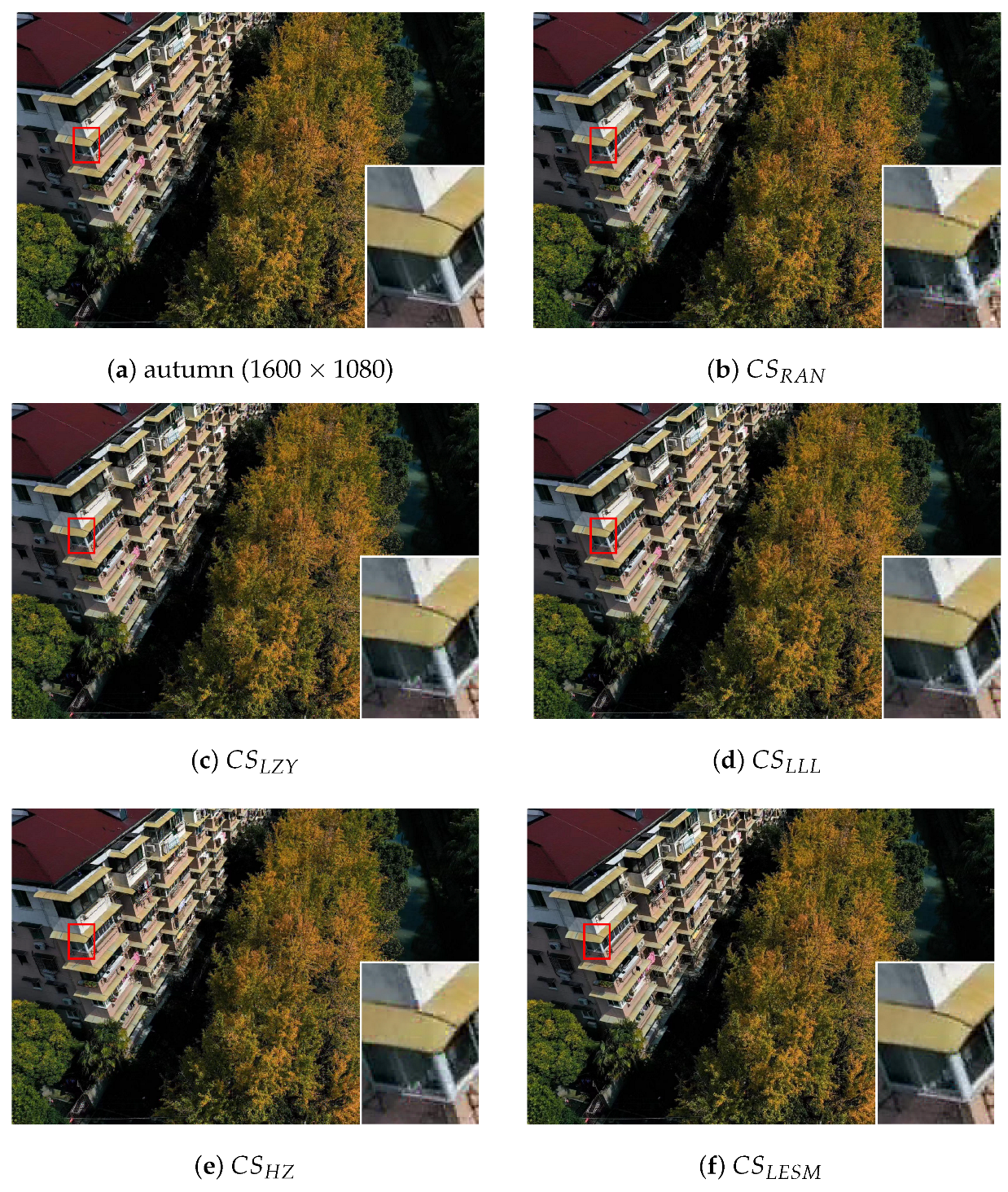
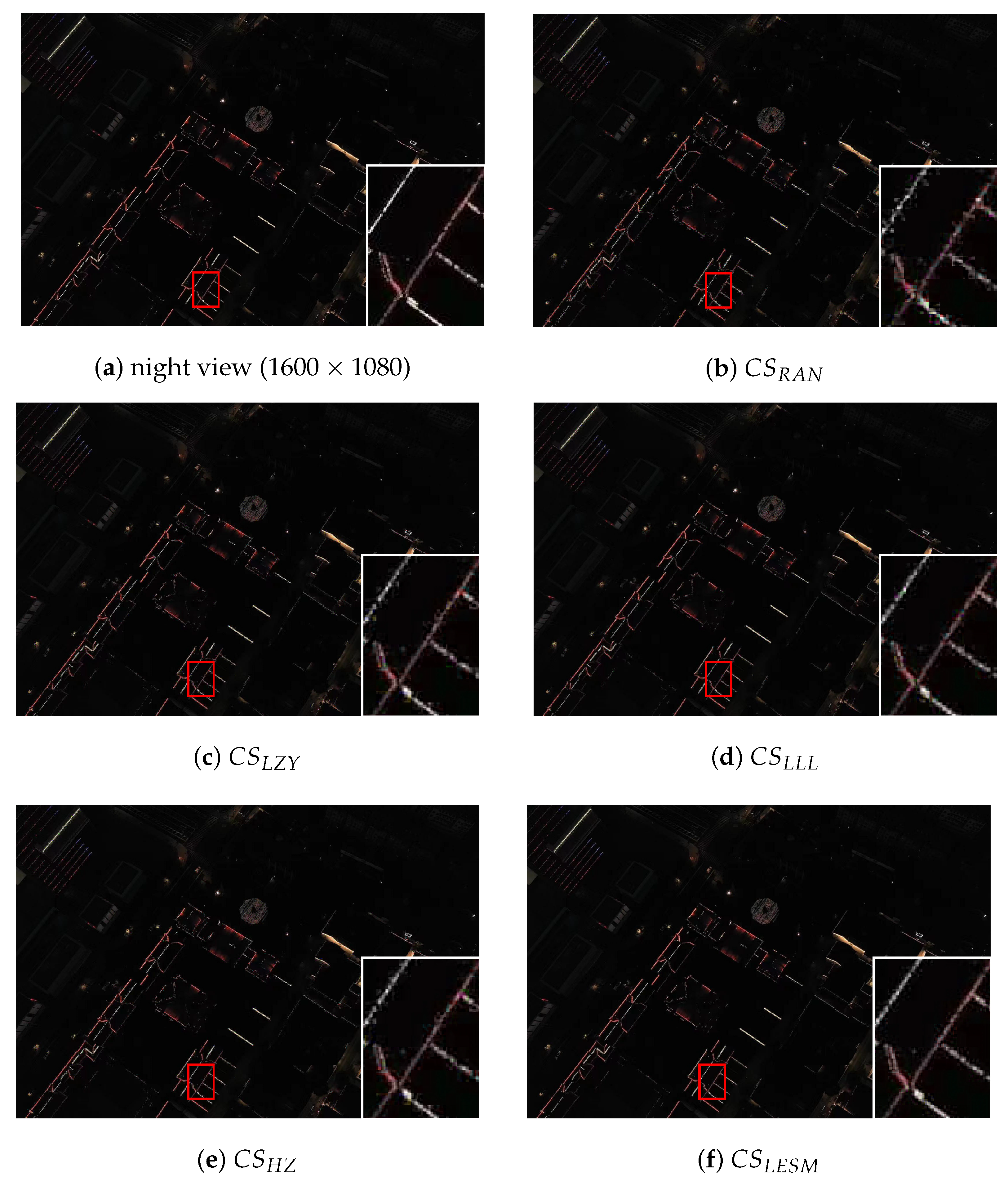
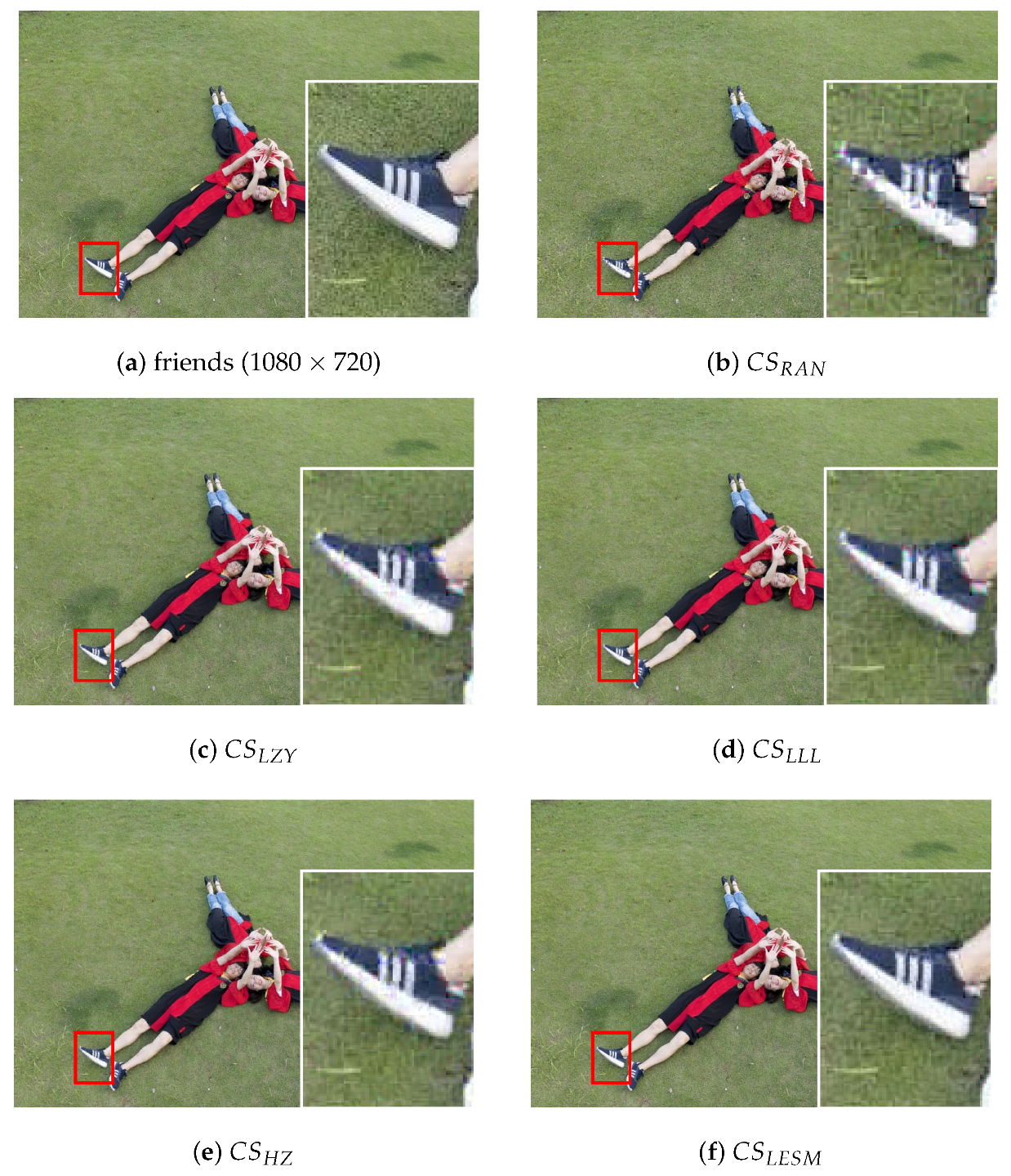
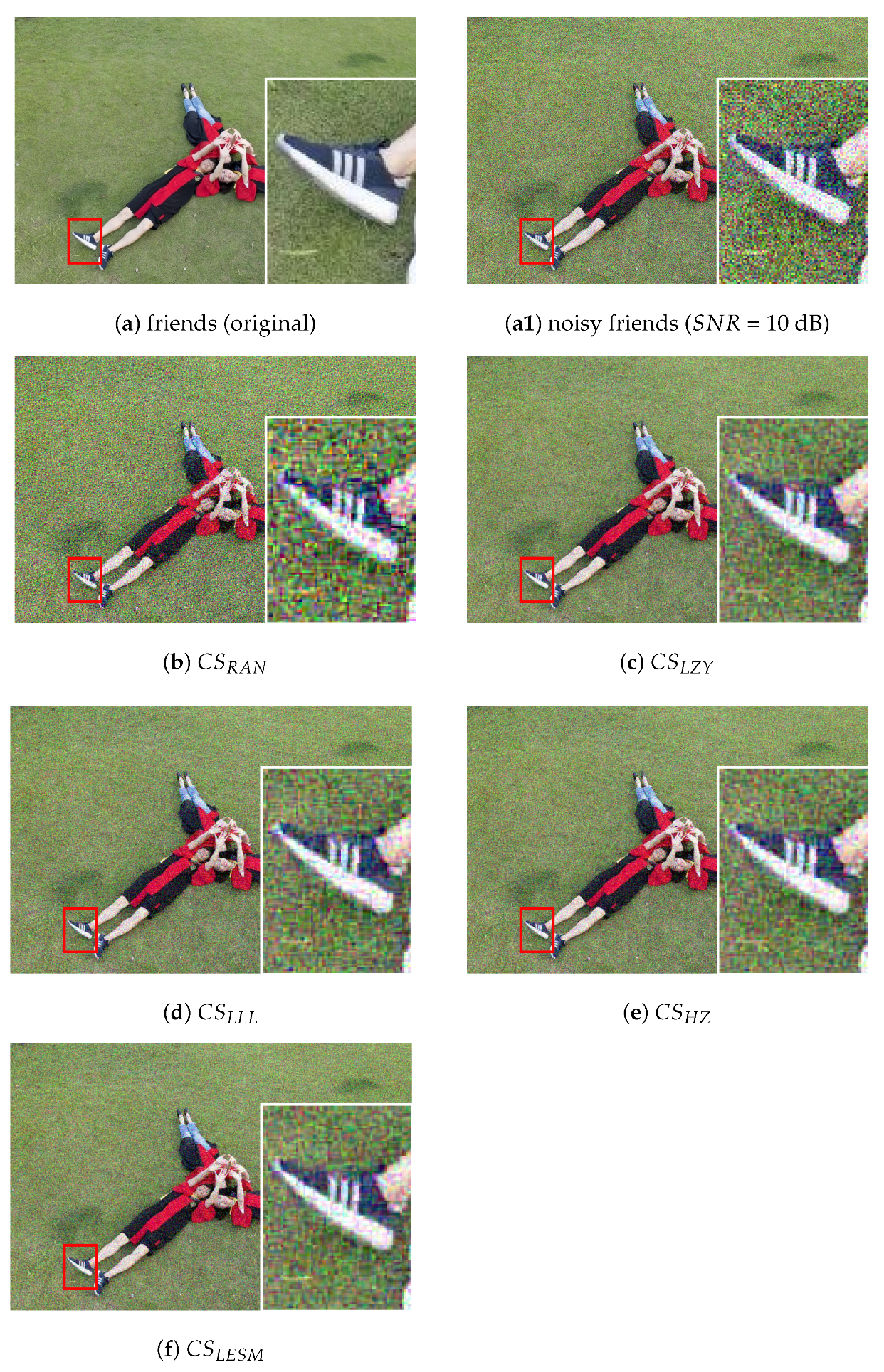
Case 4: Recovery test on UAV images taken by ourselves. We use a DJI Air 2S UAV to take images in different scenarios (“autumn”, “night view” of size 1600 × 1080 and “friends” of size 1080 × 720 ). The visual results of the above colored images are shown in Figure 3, Figure 4 and Figure 5. To observe the recovery performance more intuitively for the different algorithms, the local detail in the box is zoomed in. In addition, we test the three scenarios of images by adding the Gaussian noise of S N R = 10 dB. The visual results of the images are shown in Figure 6, Figure 7 and Figure 8. The PSNRs, SREs and SSIMs of the recovery results corresponding to the above Figures with no noise and S N R = 10 dB noise are listed in Table 4.
Remark 4.
  • Without extra noise, observe the value of PSNRs and SSIMs in Table 4 and the visual feelings in Figure 3, Figure 4 and Figure 5, where the sensing matrix algorithms C S L L L , C S H Z , and C S L E S M considering the SRE possess better recovery performance than the C S R A N , and C S L Z Y . Compared with algorithm C S L L L , the recovery accuracy of C S H Z is worse than C S L L L . The proposed algorithm C S L E S M obtains the best recovery results for these three scenarios. All the results obtained from the experiments are consistent with those theoretical analyses.
  • With adding extra noise ( S N R = 10 dB), observing the value of PSNRs and SSIMs in Table 4 and the visual feelings in Figure 6, Figure 7 and Figure 8, the sensing matrix algorithms C S L Z Y , C S L L L , and C S H Z possess a similar recovery performance. The proposed algorithm C S L E S M obtains the best recovery results for these three scenarios.
  • Compared with the original images in Figure 3a, Figure 4a, Figure 5a, Figure 6a, Figure 7a, Figure 8a and other recovery results in Figure 3b–e, Figure 4b–e, Figure 5b–e, Figure 6b–e, Figure 7b–e, Figure 8b–e, the details of recovery by adopting the proposed sensing matrix C S L E S M are the best. For instance, the corner of the building in “autumn”, the colorful light lines in “night view”, the logo of the shoes in “friends” are the clearest.
  • The images of “Night view” contain much noise by themselves due to the bad lights. Hence, the recovery results are similar with or without the extra noise. This “Night view” with more noise indicates that the recovery accuracy can be improved by reducing sparse representation errors.
  • By using the proposed algorithm C S L E S M of the sensing matrix, the experiments on both UAV123 datasets and the images taken by ourselves reveal superior recovery accuracy. The larger the noise the image contains, the more obvious the improvement space of the recovery results is.

5. Conclusions

An optimal CS framework with a new structure of SRE and design of a robust sensing matrix is proposed. The proposed structure of SRE is designed to eliminate groups of sparse representation and reduce the sparse representation error (SRE). With the lower SRE (LSRE), the model for optimizing the sensing matrix is designed by minimizing the averaged mutual coherence and the energy of the projected LSRE simultaneously, which can achieve a more robust sensing matrix. This new CS framework with the proposed sensing matrix can deal with images containing large noise, which is suitable for the application of UAV images. This designed sensing matrix is adopted in the compression and encryption of UAV images, which can lead to high accuracy recovery performance. This designed sensing matrix can guarantee efficiency and security during the transmission of UAV images.

Author Contributions

Conceptualization, Q.J.; methodology, Q.J.; software, Q.J. and H.B.; validation, Q.J. and X.H.; formal analysis, Q.J. and H.B.; investigation, X.H.; resources, X.H.; data curation, Q.J.; writing—original draft preparation, Q.J.; writing—review and editing, Q.J. and H.B.; visualization, X.H.; supervision, X.H.; project administration, Q.J.; funding acquisition, X.H. All authors have read and agreed to the published version of the manuscript.

Funding

This work was supported by the Natural Science Foundation of P.R. China (Grant: 62233016, Grant: 62222315, Grant: 61973274, Grant: 61873239, Grant: 61801159), Key Project of Natural Science Foundation of Zhejiang Province Foundation (Grant: LZ22F030007) and Key Research and Development Program of Zhejiang Province Foundation (Grant: 2020C03074).

Institutional Review Board Statement

This study does not involving humans or animals.

Informed Consent Statement

Not applicable.

Data Availability Statement

Not applicable.

Conflicts of Interest

The authors declare no conflict of interest.

References

  1. Xie, S.; Chen, Q.; Yang, Q. Adaptive Fuzzy Predefined-Time Dynamic Surface Control for Attitude Tracking of Spacecraft with State Constraints. IEEE Trans. Fuzzy Syst. 2022, 1–13. [Google Scholar] [CrossRef]
  2. Xie, S.; Chen, Q.; He, X. Predefined-Time Approximation-Free Attitude Constraint Control of Rigid Spacecraft. IEEE Trans. Aerosp. Electron. Syst. 2022, 1–11. [Google Scholar] [CrossRef]
  3. Rangappa, N.; Prasad, Y.R.V.; Dubey, S.R. LEDNet: Deep Learning-Based Ground Sensor Data Monitoring System. IEEE Sens. J. 2022, 22, 842–850. [Google Scholar] [CrossRef]
  4. Tao, M.; Chen, Q.; He, X.; Xie, S. Fixed-Time Filtered Adaptive Parameter Estimation and Attitude Control for Quadrotor UAVs. IEEE Trans. Aerosp. Electron. Syst. 2022, 58, 4135–4146. [Google Scholar] [CrossRef]
  5. Chen, Q.; Tao, M.; He, X.; Tao, L. Fuzzy Adaptive Nonsingular Fixed-Time Attitude Tracking Control of Quadrotor UAVs. IEEE Trans. Aerosp. Electron. Syst. 2021, 57, 2864–2877. [Google Scholar] [CrossRef]
  6. Cambareri, V.; Mangia, M.; Pareschi, F.; Rovatti, R.; Setti, G. On Known-Plaintext Attacks to a Compressed Sensing-Based Encryption: A Quantitative Analysis. IEEE Trans. Inf. Forensics Secur. 2015, 10, 2182–2195. [Google Scholar] [CrossRef] [Green Version]
  7. Xu, B.; Xie, Z.; Zhang, Z.; Han, T.; Liu, H.; Ju, M.; Liu, X. Joint Compression and Encryption of Distributed Sources Based on Wavelet Transform and Semi-Tensor Product Compressed Sensing. IEEE Sens. J. 2022, 22, 16451–16463. [Google Scholar] [CrossRef]
  8. Li, L.; Fang, Y.; Liu, L.; Peng, H.; Kurths, J.; Yang, Y. Overview of Compressed Sensing: Sensing Model, Reconstruction Algorithm, and Its Applications. Appl. Sci. 2020, 10, 5909. [Google Scholar] [CrossRef]
  9. Candès, E.J.; Romberg, J.; Tao, T. Robust uncertainty principles: Exact signal reconstruction from higy incomplete frequency information. IEEE Trans. Inf. Theory 2006, 52, 489–509. [Google Scholar] [CrossRef] [Green Version]
  10. Zhu, Z.; Li, G.; Ding, J.; Li, Q.; He, X. On Collaborative Compressive Sensing Systems: The Framework, Design and Algorithm. SIAM J. Imaging Sci. 2017, 11, 1717–1758. [Google Scholar] [CrossRef] [Green Version]
  11. Jalali, S. Toward Theoretically Founded Learning-Based Compressed Sensing. IEEE Trans. Inf. Theory 2020, 66, 387–400. [Google Scholar] [CrossRef]
  12. Chen, Z.; Guo, W.; Feng, Y.; Li, Y.; Zhao, C.; Ren, Y.; Shao, L. Deep-Learned Regularization and Proximal Operator for Image Compressive Sensing. IEEE Trans. Image Process. 2021, 30, 7112–7126. [Google Scholar] [CrossRef] [PubMed]
  13. Sarangi, P.; Pal, P. Measurement Matrix Design for Sample-Efficient Binary Compressed Sensing. IEEE Signal Process. Lett. 2022, 29, 1307–1311. [Google Scholar] [CrossRef]
  14. Candès, E.J.; Wakin, M.B. An introduction to compressive sampling. IEEE Signal Process. Mag. 2008, 25, 21–30. [Google Scholar] [CrossRef]
  15. Bai, H.; Li, G.; Li, S.; Li, Q.; Jiang, Q.; Chang, L. Alternating Optimization of Sensing Matrix and Sparsifying Dictionary for Compressed Sensing. IEEE Trans. Signal Process. 2015, 63, 1581–1594. [Google Scholar] [CrossRef]
  16. Pati, Y.C.; Rezaiifar, R.; Krishnaprasad, P.S. Orthogonal matching pursuit: Recursive function approximation with applications to wavelet decomposition. In Proceedings of the 2002 Asilomar Conference on Signals, Systems and Computers, Pacific Grove, CA, USA, 3–6 November 2002; Volume 1, pp. 40–44. [Google Scholar]
  17. Candès, E.J.; Tao, T. Decoding by linear programming. IEEE Trans. Inf. Theory 2005, 51, 4203–4215. [Google Scholar] [CrossRef] [Green Version]
  18. Wainwright, M.J. Sharp Thresholds for High-Dimensional and Noisy Sparsity Recovery Using 1-Constrained Quadratic Programming (Lasso). IEEE Trans. Inf. Theory 2009, 55, 2183–2202. [Google Scholar] [CrossRef]
  19. Donoho, D.L.; Elad, M. Optimally sparse representation in general (nonorthogonal) dictionaries via 1 minimization. Proc. Natl. Acad. Sci. USA 2003, 100, 2197–2202. [Google Scholar] [CrossRef] [Green Version]
  20. Li, B.; Zhang, L.; Kirubarajan, T.; Rajan, S. Projection matrix design using prior information in compressive sensing. Signal Process. 2017, 135, 36–47. [Google Scholar] [CrossRef]
  21. Strohmer, T.; Heath, R.W., Jr. Grassmannian frames with applications to coding and communication. Appl. Comp. Harmon. Anal. 2003, 14, 257–275. [Google Scholar] [CrossRef] [Green Version]
  22. Elad, M. Optimized Projections for Compressed Sensing. IEEE Trans. Signal Process. 2007, 55, 5695–5702. [Google Scholar] [CrossRef]
  23. Duarte-Carvajalino, J.M.; Sapiro, G. Learning to sense sparse signals: Simultaneous sensing matrix and sparsifying dictionary optimization. IEEE Trans. Image Process. 2009, 18, 1395–1408. [Google Scholar] [CrossRef] [PubMed] [Green Version]
  24. Li, G.; Zhu, Z.; Yang, D.; Chang, L.; Bai, H. On Projection Matrix Optimization for Compressive Sensing Systems. IEEE Trans. Signal Process. 2013, 61, 2887–2898. [Google Scholar] [CrossRef]
  25. Hong, T.; Bai, H.; Li, S.; Zhu, Z. An efficient algorithm for designing projection matrix in compressive sensing based on alternating optimization. Signal Process. 2016, 125, 9–20. [Google Scholar] [CrossRef]
  26. Bai, H.; Li, S.; He, X. Sensing Matrix Optimization Based on Equiangular Tight Frames with Consideration of Sparse Representation Error. IEEE Trans. Multimed. 2016, 18, 2040–2053. [Google Scholar] [CrossRef]
  27. Bai, H.; Hong, C.; Li, S.; Zhang, Y.D.; Li, X. Unit-norm tight frame-based sparse representation with application to speech inpainting. Digit. Signal Process. 2022, 123, 103426. [Google Scholar] [CrossRef]
  28. Li, G.; Li, X.; Li, S.; Bai, H.; Jiang, Q.; He, X. Designing robust sensing matrix for image compression. IEEE Trans. Image Process. 2015, 24, 5389–5400. [Google Scholar] [CrossRef]
  29. Li, G.; Zhu, Z.; Wu, X.; Hou, B. On joint optimization of sensing matrix and sparsifying dictionary for robust compressed sensing systems. Digit. Signal Process. 2018, 73, 62–71. [Google Scholar] [CrossRef]
  30. Hong, T.; Zhu, Z. An efficient method for robust projection matrix design. Signal Process. 2018, 143, 200–210. [Google Scholar] [CrossRef] [Green Version]
  31. Jiang, Q.; Li, S.; Chang, L.; He, X.; de Lamare, R.C. Exploiting prior knowledge in compressed sensing to design robust systems for endoscopy image recovery. J. Frankl. Inst. 2022, 359, 2710–2736. [Google Scholar] [CrossRef]
  32. Chen, Q.; Xie, S.; He, X. Neural-Network-Based Adaptive Singularity-Free Fixed-Time Attitude Tracking Control for Spacecrafts. IEEE Trans. Cybern. 2021, 51, 5032–5045. [Google Scholar] [CrossRef] [PubMed]
  33. Chen, Q.; Ye, Y.; Hu, Z.; Na, J.; Wang, S. Finite-Time Approximation-Free Attitude Control of Quadrotors: Theory and Experiments. IEEE Trans. Aerosp. Electron. Syst. 2021, 57, 1780–1792. [Google Scholar] [CrossRef]
  34. Aharon, M.; Elad, M.; Bruckstein, A. K-SVD: An algorithm for designing overcomplete dictionaries for sparse representation. IEEE Trans. Signal Process. 2006, 54, 4311–4322. [Google Scholar] [CrossRef]
  35. Zhu, Z.; Wakin, M.B. Approximating Sampled Sinusoids and Multiband Signals Using Multiband Modulated DPSS Dictionaries. J. Fourier Anal. Appl. 2015, 23, 1263–1310. [Google Scholar] [CrossRef] [Green Version]
  36. Hong, T.; Zhu, Z. Online learning sensing matrix and sparsifying dictionary simultaneously for compressive sensing. Signal Process. 2018, 153, 188–196. [Google Scholar] [CrossRef] [Green Version]
  37. Blumensath, T.; Davies, M.E. Normalized Iterative Hard Thresholding: Guaranteed Stability and Performance. IEEE J. Sel. Top. Signal Process. 2010, 4, 298–309. [Google Scholar] [CrossRef] [Green Version]
  38. Jiang, Q.; Li, S.; Zhu, Z.; Bai, H.; He, X.; de Lamare, R.C. Design of Compressed Sensing System with Probability-Based Prior Information. IEEE Trans. Multimed. 2020, 22, 594–609. [Google Scholar] [CrossRef]
  39. Liu, H.; Yuan, H.; Liu, Q.; Hou, J.; Zeng, H.; Kwong, S. A Hybrid Compression Framework for Color Attributes of Static 3D Point Clouds. IEEE Trans. Circuits Syst. Video Technol. 2022, 32, 1564–1577. [Google Scholar] [CrossRef]
  40. Mueller, M.; Smith, N.; Ghanem, B. A Benchmark and Simulator for UAV Tracking. Available online: https://cemse.kaust.edu.sa/ivul/uav123 (accessed on 13 November 2022).
  41. Gao, W.; Kwong, S.; Zhou, Y.; Yuan, H. SSIM-Based Game Theory Approach for Rate-Distortion Optimized Intra Frame CTU-Level Bit Allocation. IEEE Trans. Multimed. 2016, 18, 988–999. [Google Scholar] [CrossRef]
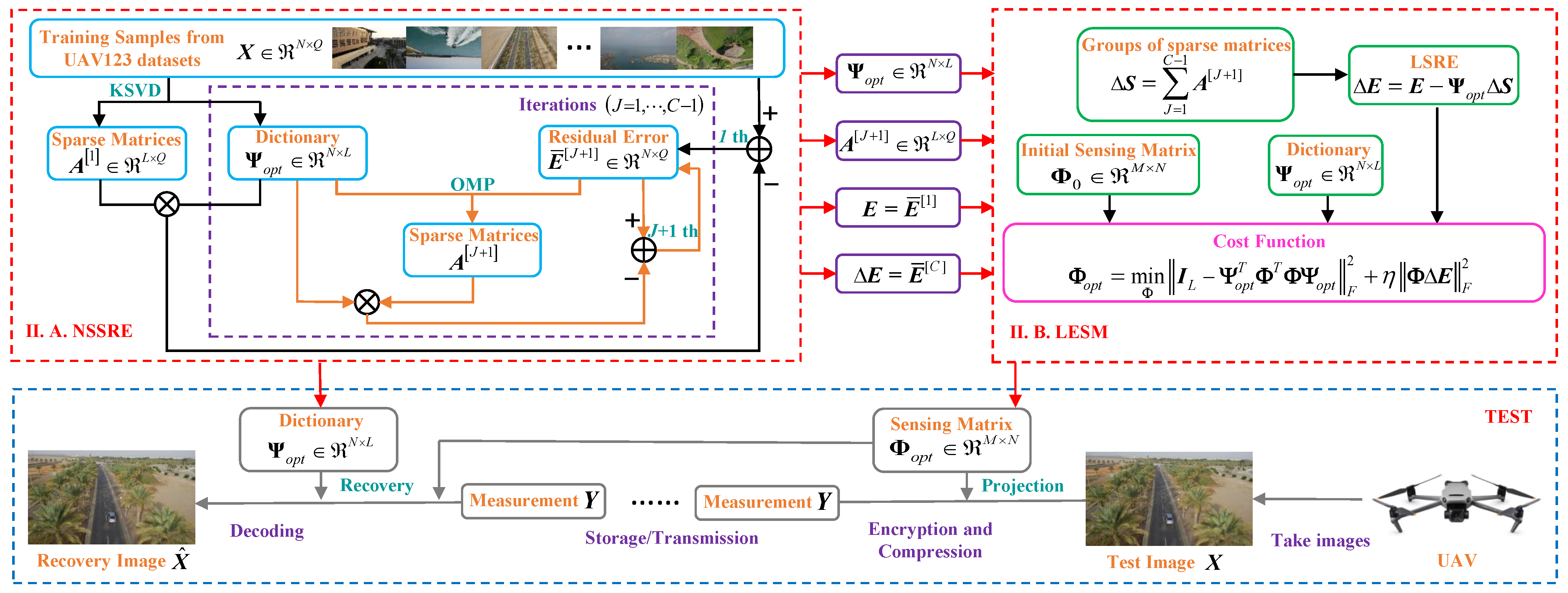
Figure 1. The CS framework of the proposed sensing matrix design (the red line) and the procedure for the UAV images compression and recovery (the blue line).
Applsci 13 01575 g001
Figure 2. The original UAV images selected randomly from each eleven classifications of the “uav123” datasets.
Applsci 13 01575 g002
Figure 3. Recovery results for the UAV image "autumn" taken by ourselves with no added noise. (a) is the original image, (b) is the C S R A N algorithm, (c) is the C S L Z Y algorithm, (d) is the C S L L L algorithm, (e) is the C S H Z algorithm, and (f) is the C S L E S M algorithm.
Applsci 13 01575 g003
Figure 4. Recovery results for the UAV image "night view" taken by ourselves with no adding noise. (a) is the original image, (b) is the C S R A N algorithm, (c) is the C S L Z Y algorithm, (d) is the C S L L L algorithm, (e) is the C S H Z algorithm, and (f) is the C S L E S M algorithm.
Applsci 13 01575 g004
Figure 5. Recovery results for the UAV image "friends" taken by ourselves with no adding noise. (a) is the original image, (b) is the C S R A N algorithm, (c) is the C S L Z Y algorithm, (d) is the C S L L L algorithm, (e) is the C S H Z algorithm, and (f) is the C S L E S M algorithm.
Applsci 13 01575 g005
Figure 6. Recovery results for the UAV image "autumn" taken by ourselves with noise ( S N R = 10 dB). (a) is the original image, (a1) is the image with noise, (b) is the C S R A N algorithm, (c) is the C S L Z Y algorithm, (d) is the C S L L L algorithm, (e) is the C S H Z algorithm, and (f) is the C S L E S M algorithm.
Applsci 13 01575 g006
Figure 7. Recovery results for the UAV image "night view" taken by ourselves with noise ( S N R = 10 dB). (a) is the original image, (a1) is the image with noise, (b) is the C S R A N algorithm, (c) is the C S L Z Y algorithm, (d) is the C S L L L algorithm, (e) is the C S H Z algorithm, and (f) is the C S L E S M algorithm.
Applsci 13 01575 g007
Figure 8. Recovery results for the UAV image "friends" taken by ourselves with noise ( S N R = 10 dB). (a) is the original image, (a1) is the image with noise, (b) is the C S R A N algorithm, (c) is the C S L Z Y algorithm, (d) is the C S L L L algorithm, (e) is the C S H Z algorithm, and (f) is the C S L E S M algorithm.
Applsci 13 01575 g008
Table 1. Performance evaluated with five sensing matrices.
Algorithm I L G F 2 Φ Δ E F 2 μ av ( D ) μ ( D )
C S R A N 6.8 × 10 5 5.68 × 10 3 0.4124 0.9874
C S L Z Y 80.0000 53.9172 0.3553 0.9359
C S L L L 83.1286 22.1217 0.3639 0.9384
C S H Z 80.3562 43.92500.35710.9387
CS LESM 82.20700.48380.36090.9443
Table 2. The PSNRs (dB), SREs and SSIMs (%) of VAU images for five sensing matrices with different M.
BikeBird
M = 20M = 24M = 20M = 24
PSNRSRESSIMPSNRSRESSIMPSNRSRESSIMPSNRSRESSIM
C S R A N 32.63 11.84 98.43 33.15 10.50 98.87 28.97 27.48 98.88 30.23 20.58 99.34
C S L Z Y 35.51 6.10 99.30 35.18 6.58 99.08 33.19 10.39 99.60 32.97 10.94 99.51
C S L L L 35.69 5.85 99.42 35.91 5.56 99.35 33.42 9.87 99.65 33.59 9.48 99.62
C S H Z 35.55 6.04 99.31 35.31 6.38 99.12 33.24 10.28 99.61 33.06 10.72 99.52
CS LESM 35.92 5.54 99.50 36.07 5.36 99.47 33.59 9.48 99.69 33.71 9.22 99.68
boatbuilding
M = 20M = 24M = 20M = 24
PSNRSRESSIMPSNRSRESSIMPSNRSRESSIMPSNRSRESSIM
C S R A N 28.14 33.29 93.99 28.73 29.05 95.56 26.39 49.74 96.17 27.08 42.43 97.25
C S L Z Y 30.71 18.41 97.06 30.46 19.50 95.79 29.16 26.27 98.22 28.87 28.09 97.52
C S L L L 31.03 17.12 97.42 31.23 16.33 97.08 29.43 24.69 98.45 29.60 23.77 98.26
C S H Z 30.74 18.28 97.11 30.56 19.04 95.96 29.19 26.10 98.25 28.99 27.38 97.62
CS LESM 31.19 16.49 97.88 31.40 15.68 97.67 29.61 23.70 98.70 29.79 22.76 98.62
cargroup
M = 20M = 24M = 20M = 24
PSNRSRESSIMPSNRSRESSIMPSNRSRESSIMPSNRSRESSIM
C S R A N 27.50 38.51 93.68 28.03 34.08 95.13 31.29 16.10 96.40 31.81 14.28 97.36
C S L Z Y 30.08 21.28 96.79 29.78 22.82 95.71 33.86 8.90 98.08 33.55 9.58 97.51
C S L L L 30.31 20.20 97.30 30.58 18.98 97.00 34.09 8.46 98.44 34.30 8.05 98.24
C S H Z 30.11 21.13 96.84 29.88 22.27 95.88 33.90 8.84 98.12 33.65 9.35 97.60
CS LESM 30.54 19.14 97.66 30.71 18.41 97.55 34.34 7.97 98.65 34.48 7.73 98.57
persontruck
M = 20M = 24M = 20M = 24
PSNRSRESSIMPSNRSRESSIMPSNRSRESSIMPSNRSRESSIM
C S R A N 37.47 3.88 96.83 38.30 3.21 97.84 33.14 10.51 98.76 33.87 8.90 99.09
C S L Z Y 40.25 2.05 98.33 40.03 2.15 97.95 36.19 5.21 99.41 35.98 5.47 99.19
C S L L L 40.55 1.91 98.67 40.88 1.77 98.51 36.49 4.86 99.50 36.69 4.64 99.44
C S H Z 40.29 2.03 98.36 40.13 2.11 98.02 36.24 5.16 99.42 36.08 5.35 99.22
CS LESM 40.84 1.79 98.80 41.03 1.71 98.75 36.61 4.73 99.56 36.78 4.55 99.54
wakebordgame
M = 20M = 24M = 20M = 24
PSNRSRESSIMPSNRSRESSIMPSNRSRESSIMPSNRSRESSIM
C S R A N 27.41 39.39 96.34 28.06 33.84 97.32 24.40 78.62 91.67 24.86 70.77 93.57
C S L Z Y 30.18 20.80 98.19 29.86 22.40 97.61 26.95 43.72 96.41 26.65 46.83 94.99
C S L L L 30.43 19.61 98.49 30.69 18.48 98.33 26.97 43.53 96.74 27.11 42.13 96.31
C S H Z 30.21 20.65 98.22 29.96 21.85 97.71 26.98 43.48 96.47 26.74 45.94 95.18
CS LESM 30.70 18.43 98.68 30.84 17.88 98.61 27.28 40.52 97.37 27.39 39.54 97.26
uavaverage
M = 20M = 24M = 20M = 24
PSNRSRESSIMPSNRSRESSIMPSNRSRESSIMPSNRSRESSIM
C S R A N 34.74 7.27 96.42 35.64 5.91 97.21 30.19 28.78 96.14 30.89 24.87 97.14
C S L Z Y 37.94 3.48 98.37 37.69 3.69 98.07 33.09 15.15 98.16 32.82 16.18 97.54
C S L L L 38.20 3.28 98.54 38.38 3.15 98.50 33.33 14.49 98.42 33.54 13.85 98.24
C S H Z 38.00 3.44 98.39 37.83 3.57 98.14 33.13 15.04 98.19 32.93 15.81 97.63
CS LESM 38.34 3.18 98.66 38.51 3.06 98.66 33.54 13.72 98.65 33.70 13.26 98.58
Table 3. The PSNRs (dB), average SRE and SSIM (%) of VAU images for five sensing matrices with different noise.
BikeBird
SNR = 20SNR = 30SNR = SNR = 20SNR = 30SNR =
PSNRSRESSIMPSNRSRESSIMPSNRSRESSIMPSNRSRESSIMPSNRSRESSIMPSNRSRESSIM
C S R A N 27.10 42.22 76.52 31.60 15.01 95.31 32.63 11.84 98.43 28.55 30.27 96.26 28.92 27.78 98.52 28.97 27.48 98.88
C S L Z Y 30.73 18.32 89.42 34.69 7.36 98.06 35.51 6.10 99.30 32.75 11.49 98.58 33.14 10.53 99.46 33.19 10.39 99.60
C S L L L 30.44 19.57 88.94 34.72 7.31 98.06 35.69 5.85 99.42 32.91 11.10 98.57 33.35 10.02 99.50 33.42 9.87 99.65
C S H Z 30.75 18.22 89.48 34.72 7.32 98.08 35.55 6.04 99.31 32.79 11.41 98.59 33.18 10.43 99.47 33.24 10.28 99.61
CS LESM 31.18 16.53 90.41 35.12 6.67 98.40 35.92 5.54 99.50 33.16 10.47 98.78 33.53 9.62 99.57 33.59 9.48 99.69
boatbuilding
SNR = 20SNR = 30SNR = SNR = 20SNR = 30SNR =
PSNRSRESSIMPSNRSRESSIMPSNRSRESSIMPSNRSRESSIMPSNRSRESSIMPSNRSRESSIM
C S R A N 25.93 55.28 81.03 27.83 35.75 92.24 28.14 33.29 93.99 24.05 85.26 82.92 26.09 53.37 94.28 26.39 49.74 96.17
C S L Z Y 29.00 27.29 91.42 30.48 19.39 96.40 30.71 18.41 97.06 27.27 40.66 92.25 28.93 27.72 97.50 29.16 26.27 98.22
C S L L L 29.03 27.09 91.35 30.75 18.23 96.67 31.03 17.12 97.42 27.26 40.75 92.11 29.15 26.38 97.67 29.43 24.69 98.45
C S H Z 29.03 27.09 91.51 30.52 19.24 96.46 30.74 18.28 97.11 27.30 40.39 92.32 28.96 27.55 7.54 29.19 26.10 98.25
CS LESM 29.49 24.37 92.78 30.96 17.37 97.30 31.19 16.49 97.88 27.75 36.43 93.25 29.37 25.04 98.06 29.61 23.70 98.70
cargroup
SNR = 20SNR = 30SNR = SNR = 20SNR = 30SNR =
PSNRSRESSIMPSNRSRESSIMPSNRSRESSIMPSNRSRESSIMPSNRSRESSIMPSNRSRESSIM
C S R A N 24.75 72.58 81.71 27.12 42.02 92.05 27.50 38.51 93.68 25.62 59.47 69.71 30.23 20.55 92.41 31.29 16.10 96.40
C S L Z Y 27.87 35.36 91.39 29.79 22.73 96.15 30.08 21.28 96.79 29.13 26.49 85.34 33.05 10.74 96.45 33.86 8.90 98.08
C S L L L 27.77 36.24 91.44 29.97 21.82 96.60 30.31 20.20 97.30 28.86 28.19 84.84 33.11 10.59 96.62 34.09 8.46 98.44
C S H Z 27.90 35.12 91.47 29.82 22.57 96.21 30.11 21.13 96.84 29.16 26.32 85.45 33.08 10.66 96.50 33.90 8.84 98.12
CS LESM 28.38 31.48 92.77 30.27 20.39 97.09 30.54 19.14 97.66 29.58 23.86 86.89 33.53 9.61 97.18 34.34 7.97 98.65
persontruck
SNR = 20SNR = 30SNR = SNR = 20SNR = 30SNR =
PSNRSRESSIMPSNRSRESSIMPSNRSRESSIMPSNRSRESSIMPSNRSRESSIMPSNRSRESSIM
C S R A N 26.45 49.08 68.21 34.11 8.41 92.58 37.47 3.88 96.83 28.03 34.10 83.95 32.14 13.24 96.57 33.14 10.51 98.76
C S L Z Y 30.23 20.57 84.42 37.36 3.98 96.55 40.25 2.05 98.33 31.68 14.73 93.02 35.39 6.27 98.59 36.19 5.21 99.41
C S L L L 29.79 22.77 83.64 37.20 4.13 96.66 40.55 1.91 98.67 31.49 15.38 92.71 35.55 6.04 98.60 36.49 4.86 99.50
C S H Z 30.25 20.47 84.49 37.40 3.94 96.60 40.29 2.03 98.36 31.71 14.63 93.05 35.43 6.21 98.60 36.24 5.16 99.42
CS LESM 30.69 18.51 85.99 37.96 3.47 97.24 40.84 1.79 98.80 32.18 13.13 93.72 35.86 5.62 98.83 36.61 4.73 99.56
wakebordgame
SNR = 20SNR = 30SNR = SNR = 20SNR = 30SNR =
PSNRSRESSIMPSNRSRESSIMPSNRSRESSIMPSNRSRESSIMPSNRSRESSIMPSNRSRESSIM
C S R A N 25.62 59.37 83.40 27.15 41.81 94.33 27.41 39.39 96.34 23.47 97.50 85.13 24.29 80.69 90.73 24.40 78.62 91.67
C S L Z Y 28.75 38.93 92.53 29.98 21.78 97.42 30.18 20.80 98.19 26.25 51.44 93.52 26.86 44.63 96.04 26.95 43.72 96.41
C S L L L 28.75 28.90 92.45 30.20 20.70 97.68 30.43 19.61 98.49 26.18 52.18 93.66 26.87 44.56 96.32 26.97 43.53 96.74
C S H Z 28.77 28.74 92.57 30.02 21.59 97.46 30.21 20.65 98.22 26.27 51.12 93.60 26.89 44.40 96.09 26.98 43.48 96.47
CS LESM 29.25 25.74 93.48 30.51 19.27 98.01 30.70 18.43 98.68 26.62 47.23 94.75 27.20 41.28 97.04 27.28 40.52 97.37
uavaverage
SNR = 20SNR = 30SNR = SNR = 20SNR = 30SNR =
PSNRSRESSIMPSNRSRESSIMPSNRSRESSIMPSNRSRESSIMPSNRSRESSIMPSNRSRESSIM
C S R A N 28.55 30.28 69.44 33.43 9.84 91.96 34.74 7.27 96.42 26.19 55.95 79.85 29.36 31.68 93.73 30.19 28.78 96.14
C S L Z Y 32.22 13.01 84.93 36.77 4.56 96.52 37.94 3.48 98.37 29.62 26.21 90.62 32.40 16.34 97.19 33.09 15.15 98.16
C S L L L 31.92 13.93 84.19 36.90 4.43 96.55 38.20 3.28 98.54 29.49 26.92 90.36 32.52 15.84 97.36 33.33 14.49 98.42
C S H Z 32.25 12.92 85.02 36.81 4.52 96.56 38.00 3.44 98.39 29.65 26.04 90.69 32.44 16.22 97.23 33.13 15.04 98.19
CS LESM 32.72 11.59 86.45 37.25 4.08 97.08 38.34 3.18 98.66 30.09 23.58 91.75 32.87 14.76 97.80 33.54 13.72 98.65
Table 4. The PSNRs (dB), SREs and SSIM (%) of VAU images taken by ourselves for five sensing matrices with different noise.
AutumnNight ViewFriends
SNR = SNR = 10SNR = SNR = 10SNR = SNR = 10
PSNRSRESSIMPSNRSRESSIMPSNRSRESSIMPSNRSRESSIMPSNRSRESSIMPSNRSRESSIM
C S R A N 22.57 119.96 93.37 21.87 140.99 88.69 29.38 25.01 98.08 29.36 25.14 98.03 26.03 54.09 84.08 16.93 439.48 31.12
C S L Z Y 24.97 69.01 97.05 24.47 77.45 95.04 32.01 13.66 99.21 32.00 13.69 99.18 28.42 31.16 93.69 20.67 185.84 51.83
C S L L L 25.23 65.00 98.12 24.47 77.36 95.28 32.20 13.05 99.52 32.04 13.54 99.34 28.55 30.25 95.00 20.27 203.86 50.28
C S H Z 25.11 66.81 97.35 24.50 76.99 95.10 32.12 13.29 99.28 32.02 13.60 99.20 28.50 30.59 94.20 20.69 185.08 51.95
CS LESM 25.33 63.52 97.96 24.84 71.11 96.11 32.32 12.72 99.47 32.31 12.75 99.45 28.65 29.59 95.22 21.05 170.28 54.36
Disclaimer/Publisher’s Note: The statements, opinions and data contained in all publications are solely those of the individual author(s) and contributor(s) and not of MDPI and/or the editor(s). MDPI and/or the editor(s) disclaim responsibility for any injury to people or property resulting from any ideas, methods, instructions or products referred to in the content.