The Cut-Off Frequency of High-Pass Filtering of Strong-Motion Records Based on Transfer Learning

Abstract

A high-pass cut-off frequency in filtering is critical to processing strong-motion records. The various processing procedures available nowadays are based on their own needs and are not universal. Regardless of the methods, a visual inspection of the filtered acceleration integration to displacement is required to determine if the selected filter passband is appropriate. A better method is to use a traversal search combined with visual inspection to determine the cut-off frequency, which is the traditional method. However, this method is inefficient and unsuitable for processing massive strong-motion records. In this study, convolutional neural networks (CNNs) were used to replace visual inspection to achieve the automatic judgment of the reasonableness of the filtered displacement time series. This paper chose the pre-trained deep neural network (DNN) models VGG19, ResNet50, InceptionV3, and InceptionResNetV2 for transfer learning, which are only trained in the fully connected layer or in all network layers. The effect of adding probability constraints on the results when predicting categories was analyzed as well. The results obtained through the VGG19 model, in which all network layers are trained and probability constraints are added to the prediction, have the lowest errors compared to the other models. The coefficient of determination (R2), root mean square error (RMSE), mean absolute error (MAE), and mean absolute percentage error (MAPE) are 0.82, 0.038, 0.026, and 2.99%, respectively.

1. Introduction

Strong-motion records provide important primary data for scientific research and engineering practice in earthquake engineering. Strong-motion records usually need to be processed scientifically and reasonably to obtain correct analysis results. Data processing is indispensable in many research subjects such as site effect analysis [1,2,3], studies on the attenuation relation of ground motion [4,5,6,7], structural design and seismic performance assessment [8,9], and seismic resilience assessment [10,11]. In structural dynamic time history analysis, appropriate natural ground motion input can effectively reduce the uncertainty in the analysis results [12,13]. However, slight baseline drift and noise in strong-motion-acceleration records will lead to significant shifts in velocity and displacement time history, which do not correspond with the physical meaning of practical earthquake events and are not appropriate for engineering input and research analysis. Therefore, it is necessary to carry out proper strong-motion records processing in earthquake engineering research.

Various methods have been proposed worldwide to process strong-motion records. The data processing method presented by the NGA strong-motion database [14,15] is firstly to remove the instrument response and zero-line offset from the acceleration time series and then to reduce the noise interference by filtering. The processing flow of the Reference database for seismic ground-motion in Europe (RESORCE) [16] is: (i) the zero-line adjustment of the acceleration time series; (ii) filtering via a fourth-order non-causal filter; (iii) polynomially fitting the baseline of the displacement time series; (iv) subtracting the second derivative of the baseline with the filtered acceleration. For the Chilean strong-motion database [17], the trigger type of all records is determined, and different methods are applied for the normal trigger and post-trigger records to taper strong-motion records before calculating the Fourier Amplitude Spectrum (FAS). The subsequent filtering process is similar to RESORCE. The data processing method proposed by the European Strong Motion Engineering Database (ESM) [18] and the Italian Strong Motion Database (ITACA) [19] is similar to the one described above. However, the zero-line correction, the taper length, the filter order, and other parameters are different, and post-processing after obtaining the filtered acceleration time series is added.

In the above processing of strong-motion records, the effects of noise are all removed by filtering, in which the high-pass and low-pass cut-off frequencies are essential parameters. For the Internet Site for European Strong-Motion Data (ISESD) [20], two constant values (0.25 Hz and 25 Hz) are used as high-pass and low-pass cut-off frequencies in band-pass filtering. In the NGA strong-motion database [14], the high-pass cut-off frequency is determined by visually examining the FAS and the integrated displacements, while the high-pass and low-pass cut-off frequencies are both determined via the visual inspection of FAS in the ESM [18] and ITACA [19]. Furthermore, in RESORCE [16], the high-pass cut-off frequency is selected by referring to the theoretical corner frequencies of the double-corner source spectrum [21], and the low-pass cut-off frequency is determined based on the recommendations of Douglas et al. [22]. In addition, the signal-to-noise ratio (SNR) can also be used to calculate the high-pass and low-pass cut-off frequencies. In the Chilean strong-motion database [17], the high-pass cut-off frequency is determined by limiting the SNR to be greater than 3.0, while the Nyquist frequency is selected as the low-pass cut-off frequency. The high-pass and low-pass cut-off frequencies were determined by limiting the SNR to be greater than 3 by Parker et al. [23]. Bahrampouri et al. [24] determined the high-pass cut-off frequency by limiting the SNR to be greater than 2, and choosing the low-pass cut-off frequency requires an SNR to be greater than 1. Edwards et al. [25] used the point at which the linear trend of the recorded FAS decays more slowly than the theoretical spectrum [26] to define the high-pass cut-off frequency. An SNR equal to 3 was taken as the lower limit of the low-pass cut-off frequency. A better method is to filter by using a high-pass cut-off frequency from small to large and to determine the rationality and accuracy of the selected high-pass cut-off frequency by visually inspecting the effect of integral displacement after filtering.

Unfortunately, low-frequency noise sometimes cannot be effectively and accurately filtered using the method above of determining the filter passband of strong-motion records. At present, a better way to ensure a high-pass cut-off frequency is to determine the rationality and accuracy of the selected cut-off frequency by visually inspecting the effect of the integral displacement after filtering, which is the traditional method [27]. If the mean value at the end of the filtered displacement time series is close to zero and the fitted straight line at the end of the range remains horizontal, the time series curve is considered qualified. A new filtered passband must be selected for filtering if it is not considered qualified. However, the efficiency of the traditional method is extremely low, and it is not suitable for processing massive strong-motion records. It is necessary to visually inspect the integral displacement after filtering to determine whether the results are acceptable.

According to Xie [28] and Zhou [29], the low-pass cut-off frequency has little effect on the baseline offset of displacement time series for strong-motion records. The low-pass cut-off frequency in this paper is taken as 35 Hz (where the sampling frequency is 100 Hz) or 20 Hz (where the sampling frequency is 50 Hz). Generally, in the traditional method, people must subjectively inspect the acceptability of the filtering result by classifying the integral displacement time series curve into qualified or unqualified. However, there is no uniform classification standard in traditional artificial identification for the integral displacement time series qualification.

Computer vision has been applied to image classification with uniform criteria and a faster speed. Convolutional neural networks (CNNs) that can automatically extract higher-dimensional features of data can significantly improve the accuracy of computer vision tasks [30,31]. However, deep neural networks (DNNs) [32] are slower to converge due to their large number of parameters. Transfer learning [33] enables the model to converge quickly by fine-tuning the pre-trained weights of the model. In this way, pre-trained network models can be better adapted to new data sets to achieve higher performance and reduce training time.

In this paper, to address the shortcomings of the traditional method, deep CNNs were used to replace visual inspection to achieve the automatic judgment of the reasonableness of a filtered displacement time series in processing massive strong-motion records. The pre-trained neural network models VGG19 [34], ResNet50 [35], InceptionV3 [36], and InceptionResNetV2 [37] were adopted for transfer learning to classify the filtered displacement time series as qualified or unqualified. The classification performance of the models that only train the fully connected layer was compared with the models in which all layers are trained. Moreover, the model with higher classification performance was applied to the traversal search of the high-pass cut-off frequency. Finally, the high-pass cut-off frequencies determined using traditional methods were used as accurate values, and four metrics widely used in past investigations (i.e., the coefficient of determination, root mean square error, mean absolute error, and mean absolute percentage error) were used to evaluate the results obtained using each model. The effect of adding a probability constraint to the predictive classification for the final results was also compared and analyzed.

2. Database

Raw ground motion records, supplied by the Center for Engineering Strong Motion Data (CESMD) [38], were adopted in this work. A total of 4461 raw records in V1c format were selected for this paper. The traditional method was applied to these raw records to obtain the appropriate high-pass cut-off frequency for each record.

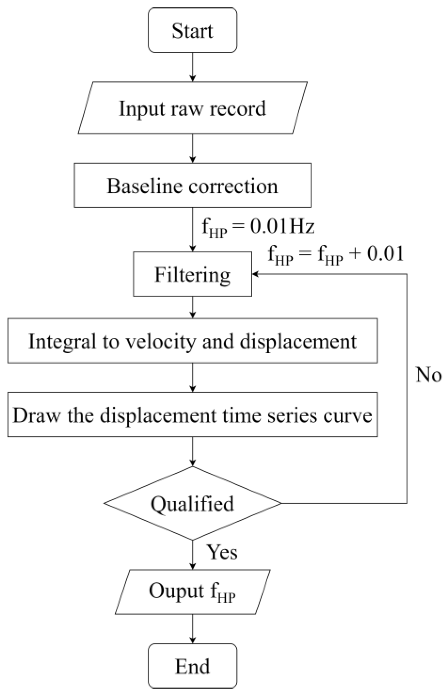
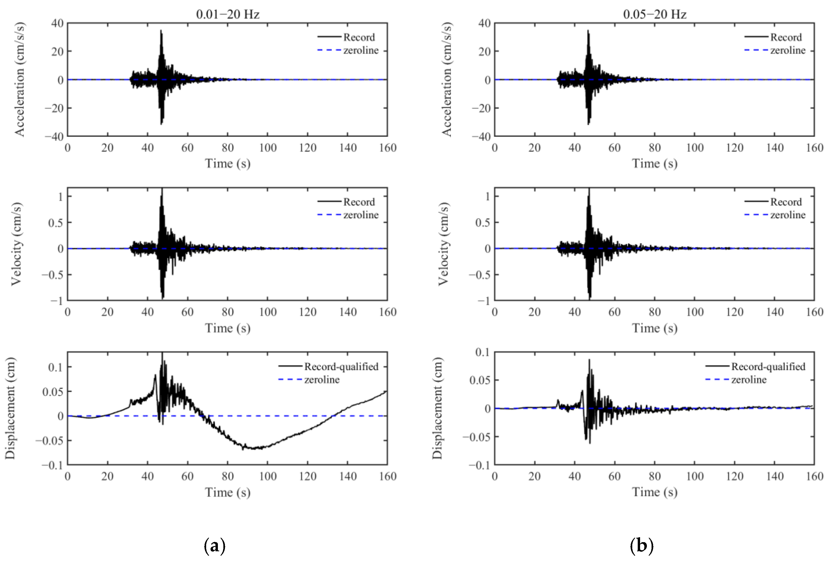
2.1. Traditional Method

The procession of the traditional method to determine the high-pass cut-off frequency of strong-motion records is shown in Figure 1, which consists of four crucial steps, as follows:

Step 1: The baseline correction of raw records. The method used here is to remove the first-order function fitted by the record.

Step 2: The selection of the appropriate high-pass cut-off frequency for filtering to remove the low-frequency noise, starting from 0.01 Hz and increasing the high-pass cut-off frequency with every step of 0.01 Hz.

Step 3: The integration of filtered acceleration time series into velocity and displacement time series.

Step 4: The artificial identification of displacement time series curves that are qualified; if they are not, skip to step 2; if they are qualified, output the cut-off frequency.

2.2. Data Pre-Processing

Yao et al. [39] showed that the causal filtering method does not produce interference signals in the noise segment before the seismic signal arrives, while acausal filtering causes interference vibration before the signal arrives. Moreover, the order of the filter is an important factor for filtering, and a higher-order filter will lead to more oscillation at both ends of the filtered record [40]. Therefore, the fourth-order Butterworth causal filter, a widely used filter [14,16,17,24,29], was used in this paper. The traditional method was used to find the high-pass cut-off frequencies of 4461 records, and 3065 records could only obtain qualified displacement time series curves only through band-pass filtering. Observing the processed records from CESMD showed that the cut-off frequencies were selected in a “one-size-fits-all” manner, i.e., the same cut-off frequency was adopted for all three components of the same record (Figure 2a). However, the velocity and displacement time series curves obtained in this way appeared to be qualified but may have had too much valid information filtered out, because the noise affecting the three components of the same record was not necessarily the same. Therefore, it was essential to find the high-pass cut-off frequency for every record. The high-pass cut-off frequencies corresponding to the 3065 records obtained using the traditional method were taken as the accurate values. The scatter plot of these values is shown in Figure 2b.

The partial acceleration, velocity, and displacement time series curves of record AKBAW--n.0212o88mof.BNE after filtering with different high-pass cut-off frequencies are shown in Figure 3. It was observed that the displacement time series curves obtained via filtering with the value before the accurate value as the cut-off frequency were all unqualified, and the ones after that were all qualified.

For each strong-motion record, up to six filtered displacement time series curves were selected for the purpose of building the database. These included three unqualified curves and three qualified curves. The three qualified displacement curves were obtained by filtering using the accurate value and two frequency values after it as the high-pass cut-off frequency. There was little difference between the displacement curves after filtering with two adjacent frequencies. The unqualified displacement curves were obtained by filtering with 0.01 Hz, 0.03 Hz, and 0.05 Hz as high-pass cut-off frequencies. The exact value of some records did not reach 0.05 Hz, so the frequency value of the unqualified time series curve was only 0.01 Hz and 0.03 Hz. A total of 8866 unqualified displacement curves and 9195 qualified displacement curves were obtained through the above method. Ultimately, 18,061 displacement curves were used as the dataset. Additionally, 80% of the data were input into the CNN as the training set, and the test and validation set was 10%; the dataset was divided randomly.

The zero line was used as a reference in the artificial identification of the drift of the displacement curve, and to facilitate machine differentiation, the zero line was represented by a solid red line. To avoid the influence of axes and legends on model training, all graphs were cropped so that the CNN could only see the displacement curve. To meet the input requirement of the networks in this paper, the image was resized to 224 × 224 × 3. The result of the image resizing is shown in Figure 4.

3. Deep Neural Networks (DNNs)

In the classification of data, convolutional neural networks (CNNs) are widely used. However, it is difficult to extract high-dimensional abstract data features in a CNN with simple architecture, and this leads to under-fitting problems. In order to achieve more effective data character extraction and classification, a more complex network model is needed. Complex network structures often have a large number of parameters, and the model takes a long time to converge. Therefore, model-based transfer learning [33] was adopted in this study to solve the above problems. Previous research [41] has shown that trained models can be adapted to other datasets or tasks by simply fine-tuning them. Fine-tuning allows the pre-trained parameters of the model to fit the new dataset better, which can improve classification performance and save training time.

3.1. Transfer Learning Model

In this paper, the VGG19 [34], ResNet50 [35], InceptionV3 [36] and InceptionResNetV2 [37] pre-trained network models were adopted for transfer learning, and the corresponding network architectures are shown in Figure 5. The parameter information regarding these models is shown in

Table 1. The parameter information regarding network models.

Model	Size (MB)	Depth	Number of Parameters (Million)
VGG19 [34]	549	26	144
ResNet50 [35]	98	168	25.6
InceptionV3 [36]	92	159	23.9
InceptionResNetV2 [37]	215	572	55.9

. It can be seen that the VGG19 network model has a minor depth but the most significant number of parameters. There are two large fully connected layers (4096 neurons) after the backbone model. Resnet50 has a global average pooling layer which dramatically reduces the size of output from the model. On the other hand, the InceptionV3 and InceptionResNetV2 models reduce the number of parameters in the model by using parallel modules and concatenating small convolutions instead of large convolutions and using a global average pooling layer.

3.2. Training and Evaluation Methods

In this paper, the training of the network model was divided into two parts. On the one hand, only the fully connected layers were trained, and the weights of all the other layers were frozen. On the other hand, all the network layers were unfrozen, and the parameters of all the network layers were fine-tuned. Additionally, all the models were trained for 50 epochs. Furthermore, Python 3.8 [42] with Tensorflow 2.8 [43] and Keras 2.8 [44] deep learning frameworks were used as the training environment. Adam [45] optimizer was used to improve the accuracy of the model. Binary cross-entropy was used as the loss function (Equation (1)). The cross-entropy function is widely used in deep learning classification, which is based on maximum likelihood estimation to fit a model. It minimizes the distance between two probability distributions (predicted and actual). Combined with the activation function in the output layer (such as sigmoid or softmax), it can accelerate the training of deep learning models faster via logarithmic operations.

Additionally, the evaluation metric $Perf$ [46] (Equation (2)) was selected to compare the performance of different models, and both training and validation performance were considered in the method.

$$\mathrm{Loss}=-\frac{1}{N}\sum _{i=1}^N{y}_i\times \log \left(p\left(y_i\right)\right)+\left(1-y_i\right)\times \log \left(1-p\left(y_i\right)\right)$$

(1)

$$Perf={\mu }_{train}\times \frac{ac{c}_{train}}{los{s}_{train}}+{\mu }_{vaild}\times \frac{ac{c}_{valid}}{los{s}_{valid}}$$

(2)

where $N$ is the total number of samples, $y_i$ is the binary label 0 or 1, and $p\left(y_i\right)$ is the probability of the output $y_i$ label. ${\mu }_{train}$ and ${\mu }_{vaild}$ are the weights of the training and validation results, respectively; the values are 0.1 and 0.9, respectively. The $ac{c}_{train}$ and $los{s}_{train}$ are the accuracy and loss of the training results, and $ac{c}_{valid}$ and $los{s}_{valid}$ are the accuracy and loss of the validation results. Here, the mean value of the last 10 epochs is presented.

3.3. Training and Evaluation Results

Figure 6 presents the detailed training process for the four network models. The solid and dashed lines are the training and validation results, respectively. Frozen denotes the models in which only the fully connected layers are trained, and unfrozen indicates the models in which all layers are trained. As shown in Figure 6, among the network models that only train fully connected layers, only the VGG19 model has higher accuracy and lower loss on the training and test sets. On the contrary, the remaining three models have relatively high losses and significantly lower and not converged accuracies. As the depth of the model increases, the accuracy of the model gets lower, and the loss gets higher and higher, indicating that the weights of other network layers except the fully connected layer are frozen so that the powerful feature extraction ability of the deep neural network has not been exerted. For the models in which all the network layers are trained, all four models achieve high accuracy in training and validation results, and the losses are close to zero and converge in the end. These results indicate that no overfitting occurred.

The performance of each model was evaluated using Equation (2), and the results are presented in

Table 2. Performance evaluation of deep transfer neural networks.

DNN	VGG19–Frozen	VGG19–Unfrozen	InceptionV3–Frozen	InceptionV3–Unfrozen	ResNet50–Frozen	ResNet50–Unfrozen	InceptionResNetV2–Frozen	InceptionResNetV2–Unfrozen
$ac{c}_{train}$	0.979	0.998	0.770	0.999	0.768	0.999	0.670	0.999
$ac{c}_{valid}$	0.980	0.997	0.801	0.997	0.801	0.997	0.682	0.998
$los{s}_{train}$	0.061	0.008	4.804	0.004	42.364	0.004	212.492	0.003
$los{s}_{valid}$	0.052	0.010	3.356	0.011	30.580	0.009	214.860	0.009
$Perf$	3.479	23.04	0.043	37.40	0.004	36.07	0.000	40.43

. For the displacement curve classification problem in this paper, the $Perf$ of InceptionV3-frozen, ResNet50-frozen, and InceptionResNetV2-frozen is close to 0, which is not suitable for this paper. However, the $Perf$ of VGG19-frozen and the model with all the network layers trained is higher, with the InceptionResNetV2-unfrozen model reaching 40.43, and they are more suitable for the dichotomous classification problem in this paper.

3.4. Test Results

Finally, the test set was tested using the network model with the lowest loss and highest accuracies among the 50 epochs. The accuracy of various models was evaluated using confusion matrices, and the corresponding results are shown in Figure 7. Categories 0 and 1 represent the unqualified and qualified displacement time curves, respectively. The diagonal elements of the matrix represent the number of samples with the correct predicted class, and the other pieces represent the number of samples with the incorrectly predicted class. The third column of the third row of the matrix is the ratio of correctly classified samples to the total number of samples, which is the accuracy rate.

As shown in Figure 7, the test results remained consistent with those in Table 2, and the InceptionResNetV2–unfrozen model performed the best with an overall accuracy of 96.9%. The five models that performed better had relatively high classification accuracies for qualified displacement curve images, with a maximum of 99.2%. For all the models, misclassifying unqualified displacement curve pictures as qualified was an essential factor affecting the overall accuracy.

In summary, among all the network models that only train the fully connected layer, the VGG19 network model has the best performance in the validation and testing process. Models with all the network layers trained can achieve good classification results. Therefore, in the following work of this paper, the VGG19–frozen model and the four models that train all the layers were chosen to identify whether the displacement curve was qualified.

4. Application of the Trained Network Models

In this section, the trained DNN models were used to identify whether the filtered displacement time curve was qualified. The artificial recognition of the displacement curve in the traditional method is replaced by a CNN, which saves a lot of time and improves work efficiency.

4.1. Filtering Results

In the filtering process of this paper, after filtering, the displacement curve changed from unqualified to qualified. When approaching the reasonable filtering frequency obtained using the traditional method, there was no significant difference in the displacement curve picture, so it would be judged as qualified prematurely. The conventional data binary classification problem considers that as long as the prediction probability is greater than 50%, it is considered to belong to the class. In order to avoid premature judgment as qualified, stricter criteria should be adopted. Therefore, probability restrictions were added to determine whether the filtered displacement curve was qualified using the deep network model. Only when a higher probability is judged to be qualified can it be considered qualified and not be the traditional 50%. After comparison, this paper argued that more than 99.9% of the probability being considered qualified is appropriate. Figure 8 and Figure 9 show the relationship between the high-pass cut-off frequency obtained by considering the probability and not considering the probability and the high-pass cut-off frequency obtained by using the traditional method when judging whether the displacement after filtering is qualified.

As seen from Figure 8 and Figure 9, almost all of these scatter points were distributed below the black line, indicating that the values obtained using the method in this paper were generally smaller than those obtained using the traditional method, and the unqualified displacement curve was prematurely judged as qualified. The black line here was y = x; if two values were equal, they were distributed on the black line.

4.2. Analysis of Filtering Results

To evaluate the accuracy of the high-pass cut-off frequencies obtained with different models, four error functions (Equations (3)–(6)) were applied to analyze the errors concerning the values obtained using the traditional method. The coefficient of determination R² is widely used in regression problems to estimate the degree of linear correlation between the true value and the predicted value. The closer R² is to 1, the better the performance of the model. The RMSE is used to measure the deviation between the predicted value and the true value. The MAE reflects the actual situation of the prediction error. The MAPE is the ratio of the prediction error to the true value. The closer these three values are to zero, the higher the performance of the model. The results of the calculations related to the four statistical parameters for each model are presented in

Table 3. Analysis of results.

Model	Considering Probability?	R2	RMSE	MAE	MAPE (%)
VGG19–frozen	Yes	0.64	0.054	0.035	21.03
	No	0.57	0.059	0.040	25.34
VGG19–unfrozen	Yes	0.82	0.038	0.026	2.99
	No	0.65	0.052	0.038	24.53
ResNet50–unfrozen	Yes	0.74	0.046	0.031	18.54
	No	0.68	0.050	0.035	21.63
InceptionV3–unfrozen	Yes	0.68	0.051	0.034	20.43
	No	0.59	0.057	0.039	24.40
InceptionResNetV2–unfrozen	Yes	0.69	0.050	0.034	20.49
	No	0.63	0.055	0.039	24.02

.

$$R^2=1-\frac{{\displaystyle \sum _{i=1}^n}{({\widehat{y}}_i-y_i)}^2}{{\displaystyle \sum _{i=1}^n}{(y_i-\overline{y})}^2}$$

(3)

$$RMSE=\sqrt{\frac{1}{n}\sum _{i=1}^n{\left({\widehat{y}}_i-y_i\right)}^2}$$

(4)

$$MAE=\frac{1}{n}\sum _{i=1}^n\left|{\widehat{y}}_i-y_i\right|$$

(5)

$$MAPE=\frac{100\%}{n}\sum _{i=1}^n\left|\frac{{\widehat{y}}_i-y_i}{y_i}\right|$$

(6)

where $y$ and $\widehat{y}$ are the high-pass cut-off frequencies obtained using the traditional method and the high-pass cut-off frequency obtained using the method of this paper, respectively, $n$ represents the number of data samples, and $\overline{y}$ denotes the mean value of $y$.

According to the analysis results in Table 3, using a CNN instead of artificial identification to judge whether a filtered displacement curve is qualified and thus obtain a high-pass cut-off frequency of strong-motion records can be satisfactory. The coefficient of determination R² reached a maximum of 0.82 and a minimum of 0.57. The RMSE ranged from a minimum of 0.038 to a maximum of 0.059. The MAE ranged from a minimum of 0.026 to a maximum of 0.040. The MAPE ranged from a maximum of 25.34% to a minimum of 2.99%. In comparison, the VGG19–unfrozen model considering probabilities was used to achieve the highest accuracy.

It can be concluded that the probability limit added to the prediction classification of the model enhanced its performance. R² was improved by an average of 14.41%, of which VGG19–unfrozen had the most improvement at 26.15%. The RMSE, MAE, and MAPE were reduced by 12.6%, 16.23%, and 30.01% on average. Among them, the three parameters of VGG19–unfrozen were reduced the most by 26.92%, 31.58%, and 87.81%. The performance of the VGG19–unfrozen model was most significantly improved by adding probabilistic restrictions.

4.3. Comparison to Results of the SNR Method

As described in the introduction, the SNR method is widely used in obtaining high-pass cut-off frequencies of strong-motion records [17,23,24,25,26]. This section compares the high-pass cut-off frequencies obtained via the traditional method in this paper with those obtained using the SNR method. The method proposed by Bahrampouri et al. [24] was used to obtain a high pass cut-off frequency, and this paper used an SNR greater than 3. The strong-motion record before the arrival of the P-wave was used as a noise window (Figure 10). The P-wave arrival pickup algorithm proposed by Ma et al. [47] was used here. The FAS of strong-motion records and noise was smoothed (the Konno–Ohmachi method [48]), and the smoothed noise FAS was linearly scaled by 4 times (the green dotted line in Figure 11). The point where the zoomed noise smoothing FAS intersects the ground motion smoothing FAS was considered the high-pass cut-off frequency (indicated by an arrow in Figure 11). The choice of a scaling factor equal to four ((signal + noise)/noise) implied an SNR equal to three as the criterion for the choice of the high-pass cut-off frequency.

Figure 12 shows the displacement curves for filtering at high-pass cut-off frequencies obtained using the traditional method, the method of this paper, and the SNR method, respectively. For this record, there was a significant drift in the filtered displacement curve using the high-pass cut-off frequency based on the SNR method, indicating that the high-pass cut-off frequency used was inappropriate.

Then, 300 records were randomly selected from the strong-motion database in this paper, and the high-pass cut-off frequencies obtained using the traditional and SNR methods were compared. Records without intersections (at 0–1 Hz range, as shown in Figure 13) between noise smoothing FAS and record smoothing FAS were removed, and 184 records could be obtained with high-pass cut-off frequencies via the SNR method. Figure 14 shows the high-pass cut-off frequencies obtained via the SNR method for 184 records.

It can be seen from Figure 14 that the high-pass cut-off frequency obtained via the SNR method was generally smaller than that obtained using the traditional method. This indicates that the displacement time series curves obtained by filtering the high-pass cut-off frequency obtained using the SNR method were mostly unqualified. In contrast, most of the displacement time series curves obtained via filtering with high-pass cut-off frequency obtained using this paper’s method were qualified.

5. Conclusions

This paper studied the rationality of using DNNs instead of artificially judging the displacement curve after filtering strong-motion records. The classification performances of the VGG19, ResNet50, InceptionV3, and InceptionResNetV2 deep transfer neural networks only training the fully connected layer and training all the layers were compared and analyzed. The trained model was then applied to high-pass cut-off frequency traverse searching. Additionally, a probability limit of 99.9% was added to the model’s classification of the qualified displacement time series. The accuracy of the high-pass cut-off frequency obtained was analyzed by using the high-pass cut-off frequency obtained via the traditional method as the accurate value. Finally, the high-pass cut-off frequencies using the SNR method were also obtained and compared with the results of the proposed method.

The main conclusions are as follows:

• Among the network models that only train the fully connected layer, only the VGG19 model could achieve satisfactory classification performance. In contrast, the rest of the models had higher losses, and the accuracies did not converge. All the trained models of all the network layers could achieve satisfactory classification performance, among which, InceptionResNetV2 had the highest performance with 99.9% and 99.8% accuracy in the training and validation sets, respectively, and 0.003 and 0.009 loss, respectively. The overall accuracy of the test set in the confusion matrix was 96.9%.
• Considering probability when predicting categories can improve the classification performance of the model. R² increased by 14.41% on average, and the RMSE, MAE, and MAPE decreased by 12.6%, 16.23%, and 30.01% on average, respectively.
• The VGG19 model with all the network layers being trained and the addition of probabilistic restrictions in predicting the category was more suitable for the high-pass cut-off frequency automatic search problem of strong-motion records in this paper. The results obtained using this model had the highest R² of 0.82 and the lowest RMSE, MAE, and MAPE of 0.038, 0.026, and 2.99%, respectively.
• The high-pass cut-off frequency obtained using the SNR method was generally smaller than the accurate value. This also inspires authors to use this frequency instead of 0.01 Hz as the starting frequency in the search for high-pass cut-off frequencies to improve efficiency.

References

1. Rong, M.; Wang, Z.; Woolery, E.W.; Lyu, Y.; Li, X.; Li, S. Nonlinear site response from the strong ground-motion recordings in western China. Soil Dyn. Earthq. Eng. 2016, 82, 99–110. [Google Scholar] [CrossRef]
2. Ren, Y.; Zhou, Y.; Wang, H.; Wen, R. Source characteristics, site effects, and path attenuation from spectral analysis of strong-motion recordings in the 2016 Kaikōura earthquake sequence. Bull. Seismol. Soc. Am. 2018, 108, 1757–1773. [Google Scholar] [CrossRef]
3. Sandhu, M.; Sharma, B.; Mittal, H.; Chingtham, P. Analysis of the Site Effects in the North East Region of India Using the Recorded Strong Ground Motions from Moderate Earthquakes. J. Earthq. Eng. 2022, 26, 1480–1499. [Google Scholar] [CrossRef]
4. Wen, R.; Xu, P.; Wang, H.; Ren, Y. Single-Station Standard Deviation Using Strong-Motion Data from Sichuan Region, China. Bull. Seismol. Soc. Am. 2018, 108, 2237–2247. [Google Scholar] [CrossRef]
5. Shoushtari, A.V.; Adnan, A.B.; Zare, M. On the selection of ground–motion attenuation relations for seismic hazard assessment of the Peninsular Malaysia region due to distant Sumatran subduction intraslab earthquakes. Soil Dyn. Earthq. Eng. 2016, 82, 123–137. [Google Scholar] [CrossRef]
6. Guo, D.; He, C.; Xu, C.; Hamada, M. Analysis of the relations between slope failure distribution and seismic ground motion during the 2008 Wenchuan earthquake. Soil Dyn. Earthq. Eng. 2015, 72, 99–107. [Google Scholar] [CrossRef]
7. Si, H.; Midorikawa, S.; Kishida, T. Development of NGA-Sub ground-motion prediction equation of 5%-damped pseudo-spectral acceleration based on database of subduction earthquakes in Japan. Earthq. Spectra 2022, 38, 2682–2706. [Google Scholar] [CrossRef]
8. Wen, R.; Ji, K.; Ren, Y. Review on selection of strong ground motion input for structural time-history dynamic analysis. Earthq. Eng. Eng. Dyn. 2019, 39, 1–18. [Google Scholar] [CrossRef]
9. Ren, Y.; Yin, J.; Wen, R.; Ji, K. The impact of ground motion inputs on the uncertainty of structural collapse fragility. Eng. Mech. 2020, 37, 115–125. [Google Scholar] [CrossRef]
10. Aroquipa, H.; Hurtado, A. Seismic resilience assessment of buildings: A simplified methodological approach through conventional seismic risk assessment. Int. J. Disaster Risk Reduct. 2022, 77, 103047. [Google Scholar] [CrossRef]
11. Narjabadifam, P.; Hoseinpour, R.; Noori, M.; Altabey, W. Practical seismic resilience evaluation and crisis management planning through GIS-based vulnerability assessment of buildings. Earthq. Eng. Eng. Vib. 2021, 20, 25–37. [Google Scholar] [CrossRef]
12. Wang, W.; Ji, K.; Wen, R.; Ren, Y.; Yin, J. Impact of strong ground motion’s process procedure on the structural nonlinear time-history analysis. Eng. Mech. 2020, 37, 42–52+62. [Google Scholar] [CrossRef]
13. Ji, K. Strong Ground Motion Selection for Multiple Levels of Seismic Fortification Demand in China. Doctor Thesis, Institute of Engineering Mechanics, China Earthquake Administration, Harbin, China, 2018. [Google Scholar]
14. Chiou, B.; Darragh, R.; Gregor, N.; Silva, W. NGA Project Strong-Motion Database. Earthq. Spectra 2019, 24, 23–44. [Google Scholar] [CrossRef] [Green Version]
15. PEER. PEER Ground Motion Database. Available online: https://ngawest2.berkeley.edu/ (accessed on 25 December 2017).
16. Akkar, S.; Sandıkkaya, M.A.; Şenyurt, M.; Azari Sisi, A.; Ay, B.Ö.; Traversa, P.; Douglas, J.; Cotton, F.; Luzi, L.; Hernandez, B.; et al. Reference database for seismic ground-motion in Europe (RESORCE). Bull. Earthq. Eng. 2013, 12, 311–339. [Google Scholar] [CrossRef] [Green Version]
17. Bastías, N.; Montalva, G.A. Chile Strong Ground Motion Flatfile. Earthq. Spectra 2016, 32, 2549–2566. [Google Scholar] [CrossRef]
18. Luzi, L.; Puglia, R.; Russo, E.; D’Amico, M.; Felicetta, C.; Pacor, F.; Lanzano, G.; Çeken, U.; Clinton, J.; Costa, G.; et al. The Engineering Strong-Motion Database: A Platform to Access Pan-European Accelerometric Data. Seismol. Res. Lett. 2016, 87, 987–997. [Google Scholar] [CrossRef] [Green Version]
19. Pacor, F.; Paolucci, R.; Ameri, G.; Massa, M.; Puglia, R. Italian strong motion records in ITACA: Overview and record processing. Bull. Earthq. Eng. 2011, 9, 1741–1759. [Google Scholar] [CrossRef]
20. Ambraseys, N.; Smit, P.; Douglas, J.; Margaris, B.; Sigbjörnsson, R.; Olafsson, S.; Suhadolc, P.; Costa, G. Internet site for European strong-motion data. Boll. Geofis. Teor. Appl. 2004, 45, 113–129. [Google Scholar]
21. Atkinson, G.M.; Silva, W. Stochastic modeling of California ground motions. Bull. Seismol. Soc. Am. 2000, 90, 255–274. [Google Scholar] [CrossRef]
22. Douglas, J.; Boore, D.M. High-frequency filtering of strong-motion records. Bull. Earthq. Eng. 2010, 9, 395–409. [Google Scholar] [CrossRef] [Green Version]
23. Parker, G.A.; Aagaard, B.T.; Hearne, M.G.; Moschetti, M.P.; Thompson, E.M.; Rekoske, J.M. The 2019 Ridgecrest, California, Earthquake Sequence Ground Motions: Processed Records and Derived Intensity Metrics. Seismol. Res. Lett. 2020, 91, 2010–2023. [Google Scholar] [CrossRef]
24. Bahrampouri, M.; Rodriguez-Marek, A.; Shahi, S.; Dawood, H. An updated database for ground motion parameters for KiK-net records. Earthq. Spectra 2020, 37, 505–522. [Google Scholar] [CrossRef]
25. Edwards, B.; Ntinalexis, M. Defining the usable bandwidth of weak-motion records: Application to induced seismicity in the Groningen Gas Field, the Netherlands. J. Seismol. 2021, 25, 1043–1059. [Google Scholar] [CrossRef]
26. Brune, J.N. Tectonic stress and the spectra of seismic shear waves from earthquakes. J. Geophys. Res. 1970, 75, 4997–5009. [Google Scholar] [CrossRef] [Green Version]
27. Yu, H.; Xu, X.; Zhang, T. Automatic Search Algorithm of Low Cut-off Frequency for Filtering Strong Motion Records. Technol. Earthq. Disaster Prev. 2018, 13, 65–74. [Google Scholar]
28. Xie, L.; Li, S.; Qian, Q.; Hu, C. Some characteristics of strong motion record processing and analysis methods in China. Earthq. Eng. Eng. Dyn. 1983, 6, 1–14. [Google Scholar] [CrossRef]
29. Zhou, B. Some Key Issues on the Strong Motion Observation. Doctor Thesis, Institute of Engineering Mechanics, China Earthquake Administration, Harbin, China, 2012. [Google Scholar]
30. Zhang, S.; Zhang, S.; Zhang, C.; Wang, X.; Shi, Y. Cucumber leaf disease identification with global pooling dilated convolutional neural network. Comput. Electron. Agric. 2019, 162, 422–430. [Google Scholar] [CrossRef]
31. Kozłowski, M.; Górecki, P.; Szczypiński, P.M. Varietal classification of barley by convolutional neural networks. Biosyst. Eng. 2019, 184, 155–165. [Google Scholar] [CrossRef]
32. Cottrell, G.W. New life for neural networks. Science 2006, 313, 454–455. [Google Scholar] [CrossRef] [Green Version]
33. Pan, S.J.; Yang, Q. A Survey on Transfer Learning. IEEE Trans. Knowl. Data Eng. 2010, 22, 1345–1359. [Google Scholar] [CrossRef]
34. Simonyan, K.; Zisserman, A. Very deep convolutional networks for large-scale image recognition. arXiv 2014, arXiv:1409.1556. [Google Scholar] [CrossRef]
35. He, K.; Zhang, X.; Ren, S.; Sun, J. Identity mappings in deep residual networks. In Proceedings of the European Conference on Computer Vision, Amsterdam, Netherlands, 8–16 October 2016; pp. 630–645. [Google Scholar]
36. Szegedy, C.; Vanhoucke, V.; Ioffe, S.; Shlens, J.; Wojna, Z. Rethinking the inception architecture for computer vision. In Proceedings of the IEEE Conference on Computer Vision and Pattern Recognition, Las Vegas, NV, USA, 27–30 June 2016; pp. 2818–2826. [Google Scholar]
37. Szegedy, C.; Ioffe, S.; Vanhoucke, V.; Alemi, A.A. Inception-v4, inception-resnet and the impact of residual connections on learning. In Proceedings of the Thirty-First AAAI Conference on Artificial Intelligence, San Francisco, CA, USA, 4–9 February 2017. [Google Scholar]
38. CESMD. Center for Engineering Strong Motion Data. Available online: https://www.strongmotioncenter.org/index.html (accessed on 20 December 2021).
39. Yao, X.; Ren, Y.; Tadahiro, K.; Wen, R.; Wang, H.; Ji, K. The procedure of filtering the strong motion record: Denoising and filtering. Eng. Mech. 2022, 39, 320–329. [Google Scholar] [CrossRef]
40. Boore, D.M. On Pads and Filters: Processing Strong-Motion Data. Bull. Seismol. Soc. Am. 2005, 95, 745–750. [Google Scholar] [CrossRef] [Green Version]
41. Yanai, K.; Kawano, Y. Food image recognition using deep convolutional network with pre-training and fine-tuning. In Proceedings of the 2015 IEEE International Conference on Multimedia & Expo Workshops (ICMEW), Turin, Italy, 29 June–3 July 2015; pp. 1–6. [Google Scholar]
42. Python. Available online: https://www.python.org/ (accessed on 15 March 2022).
43. Abadi, M.; Barham, P.; Chen, J.; Chen, Z.; Davis, A.; Dean, J.; Devin, M.; Ghemawat, S.; Irving, G.; Isard, M. {TensorFlow}: A System for {Large-Scale} Machine Learning. In Proceedings of the 12th USENIX Symposium on Operating Systems Design and Implementation (OSDI 16), Savannah, GA, USA, 2–4 November 2016; pp. 265–283. [Google Scholar]
44. Keras. The Python Deep Learning Library. Available online: https://keras.io (accessed on 15 March 2022).
45. Kingma, D.P.; Ba, J. Adam: A method for stochastic optimization. arXiv 2014, arXiv:1412.6980. [Google Scholar] [CrossRef]
46. Liao, W.; Chen, X.; Lu, X.; Huang, Y.; Tian, Y. Deep Transfer Learning and Time-Frequency Characteristics-Based Identification Method for Structural Seismic Response. Front. Built Environ. 2021, 7, 10. [Google Scholar] [CrossRef]
47. Ma, Q.; Jin, X.; Li, S.; Chen, F.; Liao, S.; Wei, Y. Automatic P-arrival detection for earthquake early warning. Chin. J. Geophys. 2013, 56, 2313–2321. [Google Scholar] [CrossRef]
48. Konno, K.; Ohmachi, T. Ground-motion characteristics estimated from spectral ratio between horizontal and vertical components of microtremor. Bull. Seismol. Soc. Am. 1998, 88, 228–241. [Google Scholar] [CrossRef]
Figure 1. The process of obtaining the high-pass cut-off frequency (fHP is the high-pass cut-off frequency).
Applsci 13 01500 g001
Figure 2. The high-pass cut-off frequency for each record. (a) CESMD; (b) traditional method.
Applsci 13 01500 g002
Figure 3. The post-filtering time series curve of record AKBAW--n.0212o88mof.BNE (d) and subsequent images are considered qualified, where figure f is the filtered time series curve using the frequency given by CESMD). (a) 0.01 Hz; (b) 0.05 Hz; (c) 0.10 Hz; (d) 0.12 Hz; (e) 0.17 Hz; (f) 0.30 Hz.
Applsci 13 01500 g003aApplsci 13 01500 g003b
Figure 4. The processing of displacement diagram. (a) Unqualified displacement time series curve; (b) qualified displacement time series curve.
Applsci 13 01500 g004
Figure 5. Architectures of typical deep neural networks. (a) VGG19; (b) ResNet50; (c) InceptionV3; (d) InceptionResNetV2.
Applsci 13 01500 g005
Figure 6. Detailed training process for deep neural networks. (a) Training and validation accuracies (frozen); (b) training and validation losses (frozen); (c) training and validation accuracies (unfrozen); (d) training and validation losses (unfrozen).
Applsci 13 01500 g006
Figure 7. Confusion matrix of test set, where green and yellow represent the number of correctly classified samples with labels of 0 and 1, respectively. (a) VGG19–frozen; (b) ResNet50–frozen; (c) InceptionV3–frozen; (d) InceptionResNetV2–frozen; (e) VGG19–unfrozen; (f) ResNet50–unfrozen; (g) InceptionV3–unfrozen; (h) InceptionResNetV2–unfrozen.
Applsci 13 01500 g007
Figure 8. The high-pass cut-off frequency was obtained using a model that only trains the fully connected layer (unit: Hz). (a) The VGG19 when not considering probability; (b) the VGG19 when considering probability.
Applsci 13 01500 g008
Figure 9. The high-pass cut-off frequency obtained by training the model of all layers (unit: Hz). (a,c,e,g) are the results of VGG19, ResNet50, InceptionV3, and InceptionResNetV2 when probabilities are not considered, respectively; (b,d,f,h) are the results of VGG19, ResNet50, InceptionV3, and InceptionResNetV2, respectively, when considering the probability.
Applsci 13 01500 g009aApplsci 13 01500 g009b
Figure 10. An example of recorded ground motion and noise (AKBAW--n.0212o88mof.BNE).
Applsci 13 01500 g010
Figure 11. Illustrative plot for selecting filter corner frequencies.
Applsci 13 01500 g011
Figure 12. Displacement curves after filtering using different cut-off frequencies.
Applsci 13 01500 g012
Figure 13. FAS of fHP cannot be obtained via SNR method (AKPWL--n.1000hyfh.HNN.--.V1c).
Applsci 13 01500 g013
Figure 14. The high-pass cut-off frequency obtained via SNR method and proposed method (unit: Hz).
Applsci 13 01500 g014