Abstract
Non-cooperative spacecraft pose acquisition is a challenge in on-orbit service (OOS), especially for targets with unknown structures. A method for the pose measurement of non-cooperative spacecrafts based on the collaboration of binocular and time-of-flight (TOF) cameras is proposed in this study. The joint calibration is carried out to obtain the transformation matrix from the left camera coordinate system to the TOF camera system. The initial pose acquisition is mainly divided into feature point association and relative motion estimation. The initial value and key point information generated in stereo vision are yielded to refine iterative closest point (ICP) frame-to-frame registration. The final pose of the non-cooperative spacecraft is determined through eliminating the cumulative error based on the keyframes in the point cloud process. The experimental results demonstrate that the proposed method is able to track the target spacecraft during aerospace missions, which may provide a certain reference value for navigation systems.
1. Introduction
The data show that nearly 2000 objects larger than 10 cm in diameter have been found in low-Earth orbit [1]. Debris not only occupies valuable orbital resources but also increases the risk of collision with orbiting satellites, resulting in the removal of space debris becoming an urgent problem [2,3,4]. The concept of OOS was proposed in the 1960s, and a great deal of research work has been carried out in this field, with more than 130 missions launched [5,6,7,8]. Since targets are in a state of free tumbling in space [9], it is necessary to determine the attitude of the target spacecraft in real time to provide accurate information for the guidance, navigation, and control (GNC) system [10], which is an indispensable condition for the acquisition of non-cooperative targets.
Monocular cameras, binocular cameras, lidar and TOF cameras are commonly used sensors in short-range detection [11]. Acquiring non-cooperative target poses by means of stereo vision has been extensively studied. Numerous studies have accomplished pose estimation by identifying docking rings and other features of satellites [12,13,14,15]. The disadvantage of an optical camera is that its imaging is greatly affected by illumination, which has certain limitations. The method based on point cloud estimation can overcome the influence of space’s complex environment. Liu et al. proposed a pose estimation method based on the known target model and the point cloud data generated by the lidar. The main advantage of this method is that the point cloud data are processed directly without the detection and tracking of features [16]. Opromolla et al. designed an approach combining the principal component analysis and template matching. The authors focused on its ability to succeed in the measurement task without any initial guess work [17]. Guo et al. presented a pose initialization based on template matching with sparse point cloud input, mainly concentrating on offline template construction [18]. However, the premise of these methods requires the CAD model on the ground experiment to achieve the pose measurement of the target satellite. In addition, due to the need for a good initial value in the point cloud registration and a weaker echo signal when the target moves at a higher speed, it is difficult to solve the problem of pose estimation based on point clouds. It is a challenge for a single sensor to reliably track a target in real time, which demonstrates the necessity of studying the pose measurement method based on multisensor collaboration.
In terms of active and passive means of collaborative navigation, Terui et al. combined stereo vision and the ICP algorithm to estimate the motion of space debris. Their work mainly focused on using time series images to cope with the disadvantages of the ICP algorithm [19]. Peng et al. designed a method to simply fuse the point cloud data reconstructed by stereo vision and the point cloud scanned through the laser radar. The extended Kalman filter algorithm was generated to acquire the pose and velocity of the non-cooperative target. However, the real-time performance needed to be improved [20]. Guo et al. proposed a target recognition algorithm based on information fusion with binocular vision and laser radar, and the attitude measurement’s accuracy was improved through a simulation experiment; however, the simulation model in this article is too simple [21]. Liu et al. proposed an accurate pose estimation method for a non-cooperative target based on a TOF camera coupled with a grayscale camera. This major work is based on 2D line and 3D line correspondence. However, some salient feature points of the target model are not considered [22]. Su et al. presented a pose tracking method for on-orbit uncooperative targets based on the deep fusion of an optical camera and laser. The authors concentrated on acquiring a dense point cloud with scale information. However, the author does not mention the elimination of cumulative errors in point cloud registration [23].
The excellence of a grayscale camera is that it can extract the details of the target with less computational effort. Active means, such as point cloud, require a large amount of computation when extracting relevant key features. Based on the advantage of two sensors, a pose estimation method based on stereo vision and point cloud tracking is proposed in this paper. The proposed method can settle the problem of initial pose acquisition and does not depend on a CAD model during spacecraft tracking. A new joint calibration method is proposed to ensure the minimum error in the conversion between different coordinate systems. A new feature point association criterion is also proposed in Section 3.2.1. The information generated in the initial pose acquisition is mapped to refine the frame-to-frame point cloud registration. Two kinds of motion experiments were performed, namely, high speed and low speed, in order to verify the feasibility of the proposed method. This method can be applied to the mission of the chaser satellite navigation systems in OOS.
The rest of this paper is organized as follows. Section 2 defines the problem of non-cooperative spacecraft pose measurement. Section 3 describes in detail the pipeline of the proposed pose estimation method. Section 4 comprises the analysis of the calibration results and the low- and high-speed experiments’ results. Section 5 summarizes the full text.
2. Problem Definition
Figure 1 presents a schematic diagram of capturing non-cooperative targets in aerospace missions. Accurate pose data are provided by the navigation system. The capturing task is completed by the robot arm at the appropriate position.
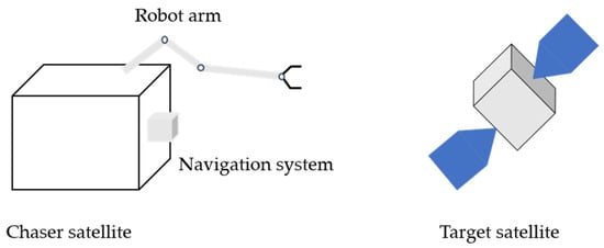
Figure 1.
Schematic diagram of the capture mission.
A schematic diagram of the composite pose measurement system built in this paper is shown in Figure 2. The visual image is acquired by grayscale cameras, and the point cloud data are acquired by a TOF camera. The projection points of the space points in the world coordinate system on the left and right camera imaging planes can be expressed as and , respectively. The left and right camera coordinate systems are and , respectively. The TOF camera coordinate system is .
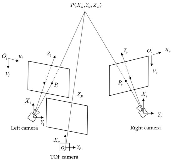
Figure 2.
Schematic diagram of the pose measurement system.
The final pose of the non-cooperative target can be determined by Equation (1).
where is the translation vector of the target spacecraft. The rotation matrix, , of non-cooperative targets in the world coordinate system can be represented by the following formula:
Then, the Euler angle of the three axes can be calculated by Equation (3).
where represent the X, Y, and Z three-axes angle transformation of the target. are the corresponding elements in the rotation matrix. The essence of solving the pose relationship of non-cooperative targets is the calculation of and .
3. Detailed Description of the Proposed Method
The specific details of the pose measurement method are presented in this section. Figure 3 illustrates the general flow of the proposed method in this study.
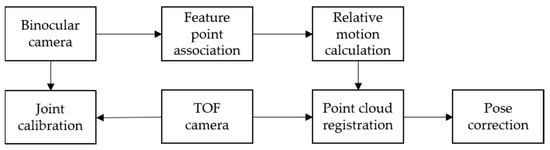
Figure 3.
Flow chart of the pose measurement algorithm for non-cooperative spacecrafts.
3.1. System Joint Calibration
Binocular system calibration is first required. Points in the left and right camera coordinate system and the world coordinate system can be represented as and , respectively. Then, the following formula is:
Combined with the above formula, there are:
where and represent the rotation matrix and translation vector from the camera coordinate system to the world coordinate system, respectively. are the external parameters of the left and right camera that need to be calculated in the binocular calibration.
The feasibility of a circular calibration board was verified in our previous work [24]. The circular calibration board is used to replace the traditional checkerboard calibration board. The center coordinates of the circle can be accurately extracted from the image. The circular calibration board is moved to different positions to acquire images that fill the entire camera field of view. Figure 4 shows the extraction results of the circular marker points on the left and right camera calibration boards.
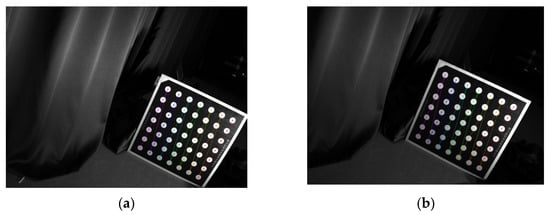
Figure 4.
The extraction results of the circle center of the calibration plate in the left and right cameras: (a) left image; (b) right image.
After completing the calibration of the binocular system, we must perform the joint calibration of the pose measurement system. The purpose of this step is to obtain the transformation relationship between the camera coordinate system and the point cloud coordinate system. It is impossible to acquire accurate three-dimensional coordinates of the circle center directly in the point cloud. Therefore, the corresponding center coordinates are yielded based on the intensity image of the TOF camera, and we map them to the point cloud coordinate system. Figure 5 illustrates the circle extraction result in the intensity image.
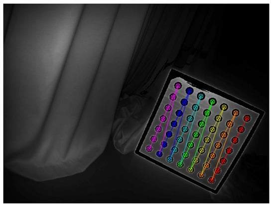
Figure 5.
The extraction result of the circle center of the calibration plate in the intensity image.
For the 2D points in the left camera image coordinate system and the corresponding 3D point in the point cloud coordinate system, the following relationship holds true:
where , and represent the joint calibration relationship to be solved. The A matrix can be represented as . The joint calibration problem becomes the problem of solving matrix A. The initial iteration value of matrix A is yielded based on the direct linear transformation (DLT). According to Formula (7):
where .
Formula (9) is then acquired:
where .
Since there are twelve variables in matrix A, at least six pairs of matching points are required to achieve the linear solution to all variables. The objective function is constructed based on the sum of the reprojection errors of the three-dimensional circle center coordinates, which can be expressed as:
where , is the homogeneous coefficient in the process of coordinate transformation, i.e., the circular center depth, . represents the L2 norm of the matrix. The Levenberg–Marquardt (LM) algorithm [25] is used to optimize the reprojection function to minimize the error function and obtain the optimal solution of the joint calibration.
3.2. Binocular Initial Pose Acquisition
The main purpose of this part is to approximately gain the motion state of the target spacecraft and provide a more accurate relative initial value for the subsequent point cloud pose estimation.
3.2.1. Feature Point Association
Common feature point extraction methods include the scale-invariant feature transform (SIFT) operator, speeded-up robust features (SURF) operator, and oriented FAST and rotated BRIEF (ORB) operator [26]. Compared with the ORB operator, the SURF operator has better robustness. Compared with the SIFT operator, it has the advantages of easier real-time processing and implementation. Overall, the SURF operator was implemented to extract the feature points in this paper. The SURF feature point response value is defined in the feature point extraction process, which represents the robustness of the feature point. The point with a small response value will be removed by calculating the response values of the feature points and sorting them.
A relatively complete feature point association criterion is proposed when tracking the target satellite in our study. As presented in Figure 6, a diagram of the feature point extraction and tracking is proposed.
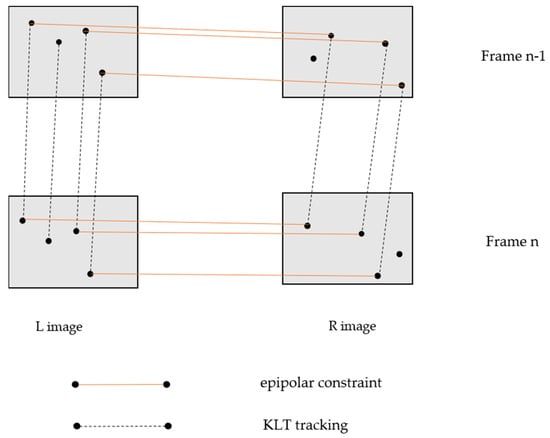
Figure 6.
Schematic diagram of the feature extraction and tracking.
The optical flow and epipolar constraint method are combined to track the feature points at the front and back moments in order to ensure the accuracy of the feature point association. In addition, the depth map obtained by the TOF camera is introduced to guide the feature point association. The depth map is projected to the left camera coordinate system through the joint calibration in Section 3.1. The disparity map of the TOF camera can be calculated with Equation (11):
where is the disparity of the TOF camera, represents the depth value, is the focal length of the left camera, and represents the baseline of the camera system.
Finally, the feature points and matched by the left and right cameras must meet the following condition:
where , which represents the disparity of the left camera. is usually set to 2. The threshold represents the disparity consistency of the feature points.
3.2.2. Relative Motion Calculation
As shown in Figure 7, the binocular initial pose estimation can be divided into the following steps.
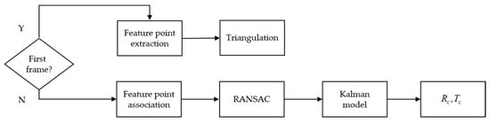
Figure 7.
Flow chart of the initial pose acquisition phase.
- (a)
- For the first frame, the feature point extraction is performed in the left and right images. A set of feature point pairs is obtained through brute force matching and the epipolar constraint criterion between the left and right cameras. Its three-dimensional coordinates in the left camera coordinate system are calculated through the principle of triangulation.
- (b)
- For a non-first frame, the number of feature points will decrease if the optical flow tracking time is too long. If the number of feature points tracked in the current frame is less than threshold (since perspective-n-point problems require at least 3 sets of points, the threshold should be greater than 3, which was set as 6 in this manuscript), then this frame adopts the method of the first frame to add new feature points. After obtaining the 3D set in the left camera coordinate system of the previous frame and the 2D feature point set of the left image in this frame, the rotation matrix and translation vector are solved quickly based on the random sample consensus (RANSAC) [27] method.
- (c)
- Since the surface of a non-cooperative spacecraft has multilayer reflective materials, the texture information is relatively lacking, which leads to the appearance of outliers in the binocular measurement process. A Kalman filter model [28] was introduced to eliminate the outliers and ensure the stability of the system in this paper.
Assuming that the acceleration of the tracking spacecraft relative to the target spacecraft is constant, the geometric kinematics between the two spacecrafts is modeled. The state and observation of the system can be represented as:
The state vector and observation vector are defined as and . and are the noise vector of the system and the noise vector in the observation process, respectively. The state transition matrix and observation matrix of the system can be defined as:
The predicted value of the filter is employed as the rotation and translation vector of the current frame to ensure that the target can still be tracked stably during the initial visual pose acquisition when abnormal values appear in the measurement process.
3.3. Point Cloud Tracking and Pose Optimization
3.3.1. Initial Value Calculation in the Point Cloud Coordinate System
In Section 3.2.2, the relative motion relationship between the front and back moments in the left camera coordinate system is acquired. We can obtain the motion relationship in the point cloud coordinate system. Assume that is the rotation matrix and translation vector in the left camera coordinate system and is the rotation matrix and translation vector from the camera coordinate system to the point cloud coordinate system obtained in the joint calibration. For a point set in space, the following motion holds at time t and t + 1:
Combined with the above formula, we obtain:
where are the rotation matrix and translation vector in the point cloud coordinate system to be solved.
3.3.2. Frame-to Frame Point Cloud Registration
The number of point clouds collected by the TOF camera is large at close range, which affects the registration speed of the point clouds at the front and back points. It is necessary to downsample the point clouds. The ICP algorithm is usually used to solve the transformation relationship between two sets of point clouds. The ICP algorithm has the disadvantage of being easily trapped in a local minimum. It is sensitive to the initial pose guess, otherwise the algorithm cannot converge on the correct result.
The standard ICP registration algorithm was used in this study. The estimated pose in stereo vision is regarded as the initial value input to improve the accuracy of the initial pose. Therefore, the initial guess of the pose variation between two datasets is provided by the binocular-based method. The feature points in stereo vision are mapped to the point cloud data and clustered to obtain several SURF-3D key points for the point cloud registration. As shown in Figure 8, the small, white squares represent the key points of SURF-3D after K-means clustering.
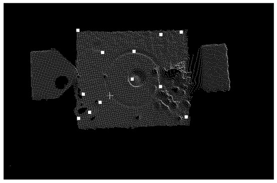
Figure 8.
Schematic Pdiagram of the point cloud with the SURF-3D key points.
The steps of the frame-to-frame point cloud registration algorithm are shown in Figure 9.
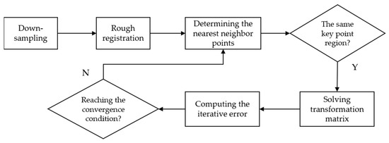
Figure 9.
Flow chart of the frame-to-frame point cloud registration algorithm.
- (a)
- Down-sampling the source point cloud using a voxel filter;
- (b)
- Using the initial pose obtained by vision to perform the initial transformation on the source point cloud and accomplishing a rough registration of the point cloud;
- (c)
- The K-dimensional tree is used to accelerate the search for point pairs between the source point cloud and the target point cloud when using the nearest neighbor to search for the corresponding points;
- (d)
- It is judged whether the points belong to the same SURF-3D key point area when using the minimum value of the Euclidean distance to determine a point pair; the false matching phenomenon is rejected.
- (e)
- The convergence condition is that the sum of the distance between the matched points is less than a given threshold or greater than the preset maximum number of iterations.
3.3.3. Pose Determination
Because of the necessity to provide a reference to the navigation system, according to our previous work, the docking ring of non-cooperative spacecraft was identified in the visual images to complete the absolute pose of the first frame. The reference absolute pose has five degrees of freedom. The detection results of the docking ring are shown in Figure 10.
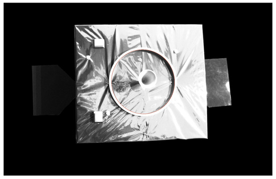
Figure 10.
The image of the docking ring detection.
The pose transformation matrix of the current i-th frame can be represented as:
where and represent the rotation matrix and the translation vector of the current frame, respectively. For the non-first frame, the pose transformation matrix of the j-th frame can be expressed as:
where represents the transformation matrix from the i-th frame point cloud to the j-th frame point cloud. A pose correction method based on key frames is proposed in this study for the purpose of eliminating the cumulative error in the process of point cloud registration and tracking. The key frames selection criteria is as follows:
(a) The frame count difference between the current frame and the previous key frame is greater than the threshold (it was set to 15 in this text), and the current frame is added to the key frame set;
(b) The relative movement distance between the current frame and the previous key frame is greater than the threshold (it was set to 100 mm in this text) or the relative angle greater than the threshold (it was set to 50 degree in this text); then, the current frame is added to the key frame set.
Inspired by the work in Reference [29], the pose objective function to be optimized in the key frame set can be defined as:
where represent the rotation matrix and translation vector from the i-th frame point cloud to the j-th frame point cloud, respectively. represents the Frobenius norm of the matrix. The abovementioned nonlinear optimization problem is solved based on the Ceres library [30] in its specific implementation.
4. Experiment and Analysis
4.1. Numerical Simulation
In the simulation setting, the image resolution of the left and right cameras was 2048 × 2048 pixels, the rotation matrix between the two cameras was , and the baseline, B, was 100 mm. The TOF resolution was 640 × 480 pixels, the rotation matrix between the left camera and TOF camera was , and the distance from left camera to the TOF camera was 50 mm.
The target rotated 180 degrees around the rolling axis in this simulation experiment. A total of 90 frames were collected. The angles of the X-, Y, and Z-axis are described as the yaw, pitch, and roll angle below, respectively. Figure 11a,b present the X-, Y-, and Z-axis position and Euler angle curve results during the low-speed rotation process.
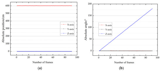
Figure 11.
Pose estimation experimental results: (a) absolute position; (b) absolute angle.
It can be concluded that the absolute transformation also represents the position error curve. The maximum error of the X-, Y-, and Z-axis positions was 0.27, 0.88, and 1.94 mm. There is no doubt that the trend of the roll angle motion was consistent with the actual situation. The maximum error of the X-, Y-, and Z-axis angles was 0.32°, 0.31°, and 0.56°.
4.2. Semi-Physical Experiments
4.2.1. Ground Verification System
A ground experiment system, as shown in the figure below, was built in order to verify the feasibility of the method proposed in this paper. The whole system included two grayscale cameras (LUCID TRI032S-MC) and one TOF camera (LUCID HLT003S-001). The grayscale camera and TOF camera parameters are shown in Table 1. The non-cooperative satellite model was a 0.5 × 0.5 m cube model. The light in the space was handled through a solar simulator.

Table 1.
Camera parameters.
The rotational movement of the target was controlled by the ABB robotic arm. The ground truth was acquired by setting the dynamic data in advance and then driving the robotic arm to complete the corresponding movement through the program in the manipulator base coordinate system. The most important thing is that the frequency of the robotic arm movement and camera system acquisition was consistent. The accuracy of the ground truth was verified by an electronic total station. The premise of this scheme is that some reflection plates need to be artificially set on the satellite model. The circular calibration board was used to acquire the conversion relationship from the total station system to the camera system. In fact, the ground truth needs to be obtained every time through the above calibration scheme. However, due to the continuous motion, the preset dynamics data are regarded as the ground truth. The diagram is shown in Figure 12. Figure 13 illustrates the ground verification system.
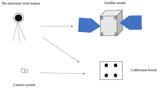
Figure 12.
Schematic diagram to verify the accuracy of the ground truth.
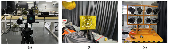
Figure 13.
Schematic diagram of the ground verification system: (a) composite measurement system; (b) diagram of the non-cooperative target; (c) solar illumination simulator.
Then, the calibration work mentioned above was carried out. The internal parameters of the left camera and right camera were:
The calibration results of the external parameters were:
According to the joint calibration algorithm proposed in this paper, the calibration results from the camera coordinate system to the point cloud coordinate system were:
The joint calibration results were verified by a reprojection experiment. As shown in Table 2, the reprojection error of the circular calibration board was much smaller than that of the checkerboard.
Table 2.
Reprojection errors of the two calibration boards.
4.2.2. Pose Measurement Experiment
The target was a specific distance from the camera system. The camera system was kept still, and the target rotated 360° under the control of the robotic arm to simulate the tumbling state of the non-cooperative target in the space environment. Several frames of visual images and point cloud were captured. Figure 14 shows the left and right camera images and the point cloud data in a specific state.
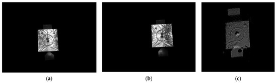
Figure 14.
Left and right camera images and TOF camera data: (a) left image; (b) right image; (c) point cloud.
Rotation Experiment at Low Speed
The target was set to a low-speed rotation rate (approximately 6 degrees per frame) in this experiment. Figure 15a,b present the X-, Y-, and Z-axis position and Euler angle curve results during the low-speed rotation process. Figure 15c,d show the X-, Y-, and Z-axis position and Euler angle error results during the rotation process.
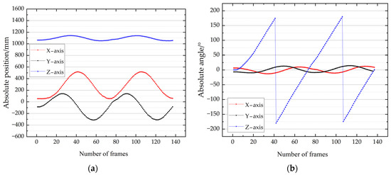
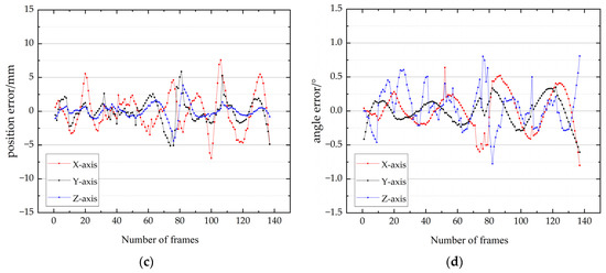
Figure 15.
Pose estimation experimental results at low speed: (a) absolute position; (b) absolute angle; (c) error of position; (d) error of angle.
Since the measurement coordinate system of the camera system was not parallel to the coordinate system of the robot arm, the X-axis and Y-axis rotated with it simultaneously when the target rolled around the Z-axis. The X-axis and Y-axis positions had a large amount of movement. Both the pitch and yaw angles had nutation of approximately 20 degrees. The maximum error and average error of the X, Y, and Z three-axis position of the proposed method was 7.6, 5.9, and 4.4 mm and 2.1, 1.4, and 0.76 mm, respectively. The maximum error and average error of the X, Y, and Z three-axis angle of the proposed method were 0.81°, 0.61°, and 0.81° and 0.22°, 0.16°, and 0.23°, respectively.
Figure 16 illustrates the X, Y, and Z three-axis position and Euler angle error results obtained by the proposed method, the stereo vision method, the traditional fast point feature histograms (FPFH) [31], and the ICP algorithm throughout the low-speed process.

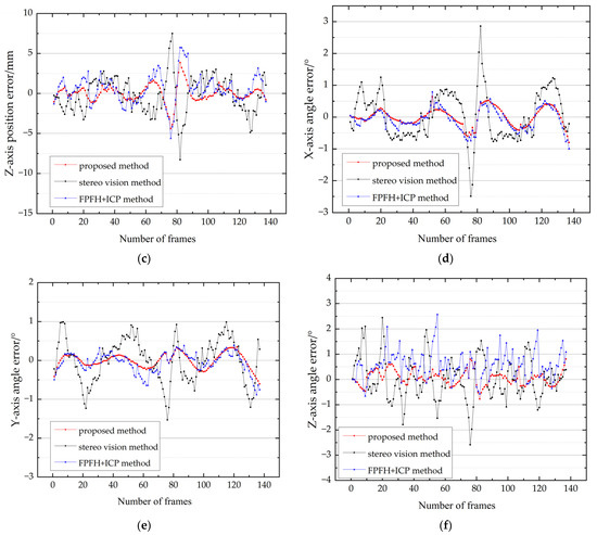
Figure 16.
Comparison of the error results of the different methods at low speed: (a) X-axis position error; (b) Y-axis position error; (c) Z-axis position error; (d) X-axis angle error; (e) Y-axis angle error; (f) Z-axis angle error.
As shown in Figure 16, it can intuitively be seen that the pose result obtained from the stereo vision method had a larger error. The maximum error and average error of the X, Y, and Z three-axis position of the stereo vision method was 24.9, 20.4, and 8.3 mm and 6.2, 7.9, and 1.8 mm, respectively. The maximum error and average error of the X, Y, and Z three-axis angle of the stereo vision method was 2.85°, 1.53°, and 2.59° and 0.66°, 0.47°, and 0.67°, respectively.
The traditional FPFH algorithm can also obtain the initial value, mainly by applying the fast point feature histogram to extract the key features, employing the initial sampling consistency registration algorithm for rough registration. The ICP fine registration and pose correction were conducted in this comparison experiment. The maximum error and average error of the X, Y, and Z three-axis position of the FPFH method was 18.3, 14.2, and 5.7 mm and 4.8, 4.0, and 1.4 mm, respectively. The maximum error and average error of the X, Y, and Z three-axis angle of the FPFH method were 0.99°, 0.88°, and 2.57° and 0.28°, 0.20°, and 0.64°, respectively.
Rotation Experiment at High Speed
The kinetic data are consistent with those in Section Rotation Experiment at Low Speed. The experimental conditions were set at a relatively high-speed rotation (approximately 12 degrees per frame). Figure 17a,b show the X-, Y-, and Z-axis position and Euler angle curve results during the high-speed rotation process. Figure 17c,d illustrate the X-, Y-, and Z-axis position and Euler angle error results during the rotation process.
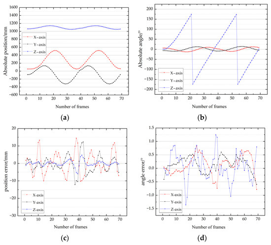
Figure 17.
Pose estimation experimental results at high speed: (a) absolute position; (b) absolute angle; (c) error of position; (d) error of angle.
The method proposed in this paper can cope with the high-speed rotation condition from the data in the figure above. The target could be tracked stably in the high-speed experiment. The maximum error and average error of the X, Y, and Z three-axis position of the proposed method were 14.4, 12.3, and 5.9 mm and 4.9, 3.5, and 1.08 mm, respectively. The maximum error and average error of the X, Y, and Z three-axis angle of the proposed method were 0.82°, 0.60°, and 1.36° and 0.29°, 0.26°, and 0.39°, respectively. Contrasted with the working conditions in Section Rotation Experiment at Low Speed, the position and angle errors increased, which still indicates that the task of capturing non-cooperative spacecrafts can be completed.
Figure 18 represents the X, Y, and Z three-axis position and Euler angle error results obtained by the proposed method, the stereo vision algorithm, and the traditional FPFH + ICP algorithm in the high-speed process.
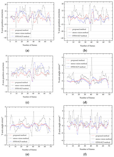
Figure 18.
Comparison of the error results of the different methods at high speed: (a) X-axis position error; (b) Y-axis position error; (c) Z-axis position error; (d) X-axis angle error; (e) Y-axis angle error; (f) Z-axis angle error.
The maximum error and average error of the X, Y, and Z three-axis position of the stereo vision method were 28.7, 30.4, 13.4 mm and 10.4, 10.4, and 3.2 mm, respectively. The maximum error and average error of the X, Y, and Z three-axis angle of the stereo vision method were 5.9°, 3.0°, and 4.6° and 0.96°, 1.01°, and 1.3°, respectively.
The error trend of the FPFH method in the high-speed rotation was coincident with the proposed method. The maximum error and average error of the X, Y, and Z three-axis position of the FPFH method were 21.3, 18.5, and 9.41 mm and 7.4, 4.8, and 3.7 mm, respectively. The maximum error and average error of the X, Y, and Z three-axis angle of the FPFH method were 1.6°, 1.21°, and 2.36° and 0.39°, 0.34°, and 0.77°, respectively.
Key Frames Threshold Selection Experiment
The selection of the key frames threshold had a great influence on eliminating the cumulative error in the process of pose measurement. Figure 19 shows the pose errors resulting from the different thresholds.
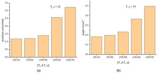
Figure 19.
The pose errors resulting from different thresholds: (a) position error; (b) angle error.
As can be seen from the figure, the selection of the key frames threshold in this manuscript was appropriate. Small thresholds will lead to more memory consumption and increase the amount of computation in the pose measurement system. The suitable thresholds Td and Ta can prevent the error drift phenomenon in the rotation process. The threshold Tc updates the set of key frames when the relative position and angle do not meet the conditions for a long time. From the perspective of memory and computation, more ground experiments are required to select the optimal threshold values in practical application.
Calculation Time Comparison of Initial Value Acquisition Methods
For a point cloud with N points and K-neighbors for each point, the computational complexity of the FPFH method is O(NK). However, the stereo vision method is O(M). M is the number of feature points. For the improved ICP point cloud registration step, the complexity of the algorithm is O(N). As shown in the figure below, the calculation times of the initial pose obtained through the proposed method and FPFH method were compared. All mentioned methods were implemented on a PC (I7-8700 at 3.2 GHz, 16 GB RAM) with Visual Studio 2019. The programming language was C++. The OPENCV library, Point Cloud Library (PCL), and Ceres optimization library were used in this study. As shown in Figure 20, the calculation time of different initial value acquisition methods are compared.
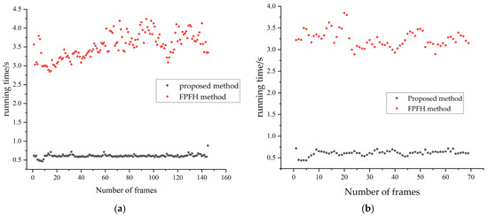
Figure 20.
Comparison of the computational time between the proposed method and the FPFH method in rotation experiments: (a) low-speed experiment; (b) high-speed experiment.
The running time of the initial pose obtained using the proposed method fluctuated around 0.6 s. However, the value acquired by the FPFH method was within 2.5 to 4.5 s. There was an improvement in the initial pose acquisition time when using the proposed method.
In summary, the relative pose error estimated in this paper was the smallest in comparison to similar experiments. The method in this paper displayed less running time, which demonstrates that it is more conducive to the application of actual control.
5. Conclusions
A method for the pose measurement of non-cooperative spacecrafts based on binocular and TOF camera collaboration was proposed. Firstly, a joint calibration method between the binocular camera and TOF camera based on a circular calibration board was conducted. The reprojection error demonstrated the effectiveness of the proposed calibration method. Then, the initial pose method was mainly divided into feature extraction, data association, and Kalman model suppression. The frame-to-frame ICP registration and pose correction based on key frames were carried out during the point cloud tracking and pose optimization. The pose results of the proposed method, stereo vision method, and the traditional FPFH method were compared in the ground verification experiment. The experimental results show that the position error of the proposed method was within 1 cm, and the angle error was within 1 degree in a low-speed rotation process. The position and angle error were within 1.5 cm and 1.4 degrees during the high-speed rotation conditions, respectively. The proposed method had a certain accuracy and robustness when chasing the target satellite, especially for a satellite with an unknown structure. In further studies, the relative orbital and attitude dynamics should be considered in the Kalman filtering process, and the proposed method should be implemented on the embedded platform to verify the real-time performance.
Author Contributions
Conceptualization, L.H. and H.D.; methodology, L.H. and D.S.; Validation, L.H., D.S. and A.S.; formal analysis, S.Z.; investigation, H.P.; resources, H.P.; data curation, L.H., D.S. and A.S.; writing—original draft preparation, L.H.; writing—review and editing, D.S. and H.D.; supervision, S.Z.; funding acquisition, H.P. All authors have read and agreed to the published version of the manuscript.
Funding
This research was funded by the Preliminary Research Foundation of Equipment, grant number: 3050404030, and the Innovation Program CX-325 of the Shanghai Institute of Technical Physics.
Institutional Review Board Statement
Not applicable.
Informed Consent Statement
Not applicable.
Data Availability Statement
Not applicable.
Conflicts of Interest
The authors declare no conflict of interest.
References
- Takeichi, N.; Tachibana, N. A tethered plate satellite as a sweeper of small space debris. Acta Astronaut. 2021, 189, 429–436. [Google Scholar] [CrossRef]
- Muntoni, G.; Montisci, G.; Pisanu, T.; Andronico, P.; Valente, G. Crowded Space: A Review on Radar Measurements for Space Debris Monitoring and Tracking. Appl. Sci. 2021, 11, 1364. [Google Scholar] [CrossRef]
- Razzaghi, P.; Al Khatib, E.; Bakhtiari, S.; Hurmuzlu, Y. Real time control of tethered satellite systems to de-orbit space debris. Aerosp. Sci. Technol. 2021, 109, 106379. [Google Scholar] [CrossRef]
- Mark, C.P.; Kamath, S. Review of active space debris removal methods. Space Policy 2019, 47, 194–206. [Google Scholar] [CrossRef]
- Liu, J.; Tong, Y.; Liu, Y.; Liu, Y. Development of a novel end-effector for an on-orbit robotic refueling mission. IEEE Access. 2020, 8, 17762–17778. [Google Scholar] [CrossRef]
- Li, W.; Cheng, D.; Liu, X.; Wang, Y.; Shi, W.; Tang, Z.; Gao, F.; Zeng, F.; Chai, H.; Luo, W.; et al. On-orbit service (OOS) of spacecraft: A review of engineering developments. Prog. Aerosp. Sci. 2019, 108, 32–120. [Google Scholar] [CrossRef]
- Moghaddam, B.M.; Chhabra, R. On the guidance, navigation and control of in-orbit space robotic missions: A survey and prospective vision. Acta Astronaut. 2021, 184, 70–100. [Google Scholar]
- Luu, M.A.; Hastings, D.E. On-Orbit Servicing System Architectures for Proliferated Low-Earth-Orbit Constellations. J. Spacecr. Rocket. 2022, 59, 1946–1965. [Google Scholar] [CrossRef]
- Oestreich, C.; Espinoza, A.T.; Todd, J.; Albee, K.; Linares, R. On-Orbit Inspection of an Unknown, Tumbling Target Using NASA’s Astrobee Robotic Free-Flyers. In Proceedings of the IEEE/CVF Conference on Computer Vision and Pattern Recognition, Nashville, TN, USA, 20–25 June 2021; pp. 2039–2047. [Google Scholar]
- Huang, X.; Li, M.; Wang, X.; Hu, J.; Zhao, Y.; Guo, M.; Xu, C.; Liu, W.; Wang, Y.; Hao, C.; et al. The Tianwen-1 guidance, navigation, and control for Mars entry, descent, and landing. Space Sci.Technol. 2021, 2021, 9846185. [Google Scholar]
- Zhao, G.; Xu, S.; Bo, Y. LiDAR-based non-cooperative tumbling spacecraft pose tracking by fusing depth maps and point clouds. Sensors 2018, 18, 3432. [Google Scholar] [CrossRef]
- Hu, Q.; Jiang, C. Relative Stereovision-Based Navigation for Noncooperative Spacecraft via Feature Extraction. IEEE/ASME Trans. Mechatron. 2022, 27, 2942–2952. [Google Scholar] [CrossRef]
- Zhang, L.; Zhu, F.; Hao, Y.; Pan, W. Rectangular-structure-based pose estimation method for non-cooperative rendezvous. Appl. Opt. 2018, 57, 6164–6173. [Google Scholar] [CrossRef] [PubMed]
- Peng, J.; Xu, W.; Liang, B.; Wu, A. Virtual stereovision pose measurement of noncooperative space targets for a dual-arm space robot. IEEE Trans. Instrum. Meas. 2019, 69, 76–88. [Google Scholar] [CrossRef]
- Li, Y.; Jia, Y. Stereovision-based Relative Motion Estimation Between Non-cooperative spacecraft. In Proceedings of the 2019 Chinese Control Conference (CCC), Guangzhou, China, 27–30 July 2019; pp. 4196–4201. [Google Scholar]
- Liu, L.; Zhao, G.; Bo, Y. Point cloud based relative pose estimation of a satellite in close range. Sensors 2016, 16, 824. [Google Scholar] [CrossRef] [PubMed]
- Opromolla, R.; Fasano, G.; Rufino, G.; Grassi, M. Pose estimation for spacecraft relative navigation using model-based algorithms. IEEE Trans. Aerosp. Electron. Syst. 2017, 53, 431–447. [Google Scholar] [CrossRef]
- Guo, W.; Hu, W.; Liu, C.; Lu, T. Pose initialization of uncooperative spacecraft by template matching with sparse point cloud. J. Guid. Control Dyn. 2021, 44, 1707–1720. [Google Scholar] [CrossRef]
- Terui, F.; Kamimura, H.; Nishida, S. Motion estimation to a failed satellite on orbit using stereo vision and 3D model matching. In Proceedings of the 2006 9th International Conference on Controll, Automation, Robotics and Vision, Singapore, 5–8 December 2006; pp. 1–8. [Google Scholar]
- Peng, J.; Xu, W.; Liang, B.; Wu, A. Pose measurement and motion estimation of space non-cooperative targets based on laser radar and stereo-vision fusion. IEEE Sens. J. 2018, 19, 3008–3019. [Google Scholar] [CrossRef]
- Guo, P.; Zhang, Y.; Hu, Q. Pose Measurement of Non-cooperative Spacecraft by Sensors Fusion. In Proceedings of the 2022 41st Chinese Control Conference (CCC), Hefei, China, 25–27 July 2022; pp. 3426–3431. [Google Scholar]
- Liu, Z.; Liu, H.; Zhu, Z.; Song, J. Relative pose estimation of uncooperative spacecraft using 2D–3D line correspondences. Appl. Opt. 2021, 60, 6479–6486. [Google Scholar] [CrossRef]
- Su, Y.; Zhang, Z.; Wang, Y.; Yuan, M. Accurate Pose Tracking for Uncooperative Targets via Data Fusion of Laser Scanner and Optical Camera. J. Astronaut. Sci. 2022, 1–19. [Google Scholar]
- Sun, D.; Hu, L.; Duan, H.; Pei, H. Relative Pose Estimation of Non-Cooperative Space Targets Using a TOF Camera. Remote Sens. 2022, 14, 6100. [Google Scholar] [CrossRef]
- Vidmar, A.; Brilly, M.; Sapač, K.; Kryžanowski, A. Efficient Calibration of a Conceptual Hydrological Model Based on the Enhanced Gauss–Levenberg–Marquardt Procedure. Appl. Sci. 2020, 10, 3841. [Google Scholar] [CrossRef]
- Zhang, G.; Qin, D.; Yang, J.; Yan, M.; Tang, H.; Bie, H.; Ma, L. UAV Low-Altitude Aerial Image Stitching Based on Semantic Segmentation and ORB Algorithm for Urban Traffic. Remote Sens. 2022, 14, 6013. [Google Scholar] [CrossRef]
- Fischler, M.A.; Bolles, R.C. Random sample consensus: A paradigm for model fitting with applications to image analysis and automated cartography. Commun. ACM 1981, 24, 381–395. [Google Scholar] [CrossRef]
- Urrea, C.; Agramonte, R. Kalman filter: Historical overview and review of its use in robotics 60 years after its creation. J. Sensors 2021, 2021, 9674015. [Google Scholar] [CrossRef]
- Wang, Q.; Cai, G. Pose estimation of a fast tumbling space noncooperative target using the time-of-flight camera. Proc. Inst. Mech. Eng. Part G J. Aerosp. Eng. 2021, 235, 2529–2546. [Google Scholar] [CrossRef]
- Agarwal, S.; Mierle, K. Ceres solver: Tutorial & reference. Google Inc. 2012, 2, 8. [Google Scholar]
- Rusu, R.B.; Blodow, N.; Beetz, M. Fast point feature histograms (FPFH) for 3D registration. In Proceedings of the 2009 IEEE international conference on robotics and automation, Kobe, Japan, 12–17 May 2009; pp. 3212–3217. [Google Scholar]


Disclaimer/Publisher’s Note: The statements, opinions and data contained in all publications are solely those of the individual author(s) and contributor(s) and not of MDPI and/or the editor(s). MDPI and/or the editor(s) disclaim responsibility for any injury to people or property resulting from any ideas, methods, instructions or products referred to in the content. |
© 2023 by the authors. Licensee MDPI, Basel, Switzerland. This article is an open access article distributed under the terms and conditions of the Creative Commons Attribution (CC BY) license (https://creativecommons.org/licenses/by/4.0/).