Abstract
The pseudo-static method was adopted to expand the application field of classical Rankine soil pressure theory to the circumstance of infinite inclined backfill acting on the retaining wall under earthquakes. The calculation formula of the active earth pressure for unsaturated soil was deduced by combining the shear strength model of unsaturated soil and the unified strength theory. The effects of matric suction, matric-suction-related friction angle and seismic coefficients on the intensity distribution of Rankine active earth pressure were evaluated, and the resultant action position was discussed. This research shows that rising seismic coefficients lead to a growth of the active earth pressure and an upward movement of the resultant action point; on the other hand, an increasing matric suction and its related friction angle causes a reduction of the active earth pressure and a downward movement of the resultant action. Examples indicate that the suggested formulas in this paper are in good agreement with those of the previous literature subjected to certain conditions. However, compared to the classic Rankine theory, the proposed method extends its application range by considering earthquake, unsaturated soil, inclined rough wall back, non-horizontal backfill surface, and the intermediate principal stress.
1. Introduction
The earth pressure of retaining structures has remained an important issue in geotechnical engineering [1,2]. Meanwhile, the evaluation of earth pressure under seismic or unsaturated conditions is an important part of the design for retaining structures. As a classical theory widely used in earth pressure calculation, the Rankine theory has been extended to the field of unsaturated soil in recent years. Pufahl analyzed the lateral earth pressures of a retaining wall produced by saturated clays with negative pore-water pressures and unsaturated expansive clays with positive matric suctions [3]. Fu et al. [4] took the vertical rigid retaining wall with a narrow unsaturated backfill as the research object. By assuming that the backfill behind the wall forms a circular soil arch, the analytical solution of the active earth pressure of narrow unsaturated soil was derived based on the thin layer element method. Based on Fredlund’s shear strength criterion for unsaturated soils and the Rankine earth pressure theory, Ren and Yao proposed the calculation methods for unsaturated earth pressure [5,6]. Zhang was concerned with the nonlinearity of unsaturated soils strength and its influence on passive earth pressure, and proposed the parameter determination approach [7]. By combining the Rankine earth pressure formula of unsaturated soil and Iverson’s analytic solution of rainfall infiltration, the formula for the earth pressure of unsaturated soils under rainfall was concluded [8]. Furthermore, in order to consider the effect of intermediate principal stress, the Rankine earth pressure calculation method was modified according to the twin shear unified strength theory [9]. The unified solution of unsaturated Rankine earth pressure under rainfall conditions was put forward with the consideration of intermediate principal stress and the tension–compression ratio of the soil [10]. Additionally, based on the unified strength theory and the shear strength criterion of unsaturated soils with two stress state variables, the unified solutions of shear strength and earth pressure of unsaturated soil were obtained [11].
In recent years, significant progress has been achieved in the research of seismic earth pressure. For instance, Rankine earth pressure was extended to seismic circumstance by the use of the quasi-static method, though it was only applicable for the case of non-cohesive backfill and vertical border with the retaining wall [12]. Lin and Sun adopted the horizontal layer analysis method to acquire the stress distribution and the location of resultant earth pressure under seismic conditions, limited to the horizontal backfill surface and saturated soils [13,14]. Based on the classic Coulomb earth pressure theory, the seismic active earth pressure in the pseudo-static state was converted to non-seismic active earth pressure by using the transformation approach of rotating the retaining wall model [15]. In order to investigate the response spectrum characteristics of the dynamic soil pressure along the elevation and sliding surface of loess slopes under the action of earthquake, large-scale shaking table experiments were performed by progressively loading X-direction and Z-direction seismic waves until failure of the slope. The dynamic soil pressure curves of five sensors along the elevation and near the sliding surface were obtained, and the time–domain curve of the dynamic soil pressure was decomposed by using wavelet transform [16]. Based on the plane strain unified strength theory formula, while also considering the soil arching effects and tension cracks, the analytical solutions of the lateral earth pressure coefficient and the active earth pressure under the earthquake action were deduced by Liu et al. [17], and the mechanism and distribution of seismic active earth pressure with a limited width were discussed in terms of some relevant parameters.
It could be seen that the generalized approach of seismic active earth pressure for unsaturated soil is still lacking in research. Aiming at further broadening the application range of Rankine’s earth pressure theory and clarifying the variation characteristics of the seismic active earth pressure of unsaturated filling, a unified shear strength solution with two stress state variables for unsaturated soil and the pseudo-static method were employed to obtain the generalized calculation method of the seismic active earth pressure of unsaturated backfill, taking inclined rough wall back and non-horizontal backfill surface into consideration. Furthermore, the distribution and resultant action position of seismic active earth pressure were illustrated.
2. Principals and Methods
2.1. Unified Shear Strength of Unsaturated Soil
The shear strength of unsaturated soils is one of the basic problems in unsaturated soil mechanics. Much research has been carried out and various calculation formulas have been suggested [18,19]. However, based on Mohr-Coulomb strength theory, these formulas cannot reflect the effect of intermediate principal stress. Consequently, they cannot fully estimate the strength potential and self-supporting capacity of unsaturated backfills.
The unified strength theorem and the calculation formula of unsaturated soil could be denoted as follows [11]:
where
In the above equations, F and F′ are yield functions under different stress conditions, σ denotes the total normal stress, σ1, σ2 and σ3 represent the principal stresses and σ1 ≥ σ2 ≥ σ3; ua, uw are the pore air pressure and pore water pressure. Variables σt and σc are the tensile strength and compressive strength of the filling; τf is the shear strength of unsaturated soil; c′ and φ′ are the effective cohesion and effective friction angle of the saturated soil, respectively; (σ − ua) is the net normal stress acting on the sliding surface; (ua − uw) is the matric suction on the sliding surface; φb is the friction angle attributed by the matric suction; c′t and φ′t are the unified effective cohesion and unified effective friction angle, respectively; φbt represents the unified friction angle attributed by the matric suction; and b is the unified strength factor (0 ≤ b ≤ 1). The lower bound b = 0 refers to the Mohr-Coulomb strength criterion. On the contrary, the upper bound b = 1 refers to the twin shear strength theory. It can be obtained by fitting Equation (2) with the true triaxial test results.
Rewriting Equation (2), we get
in which the apparent cohesion ctt is
2.2. Pseudo-static Analysis of Seismic Active Earth Pressure
2.2.1. Stress Analysis of The Rhombic Element
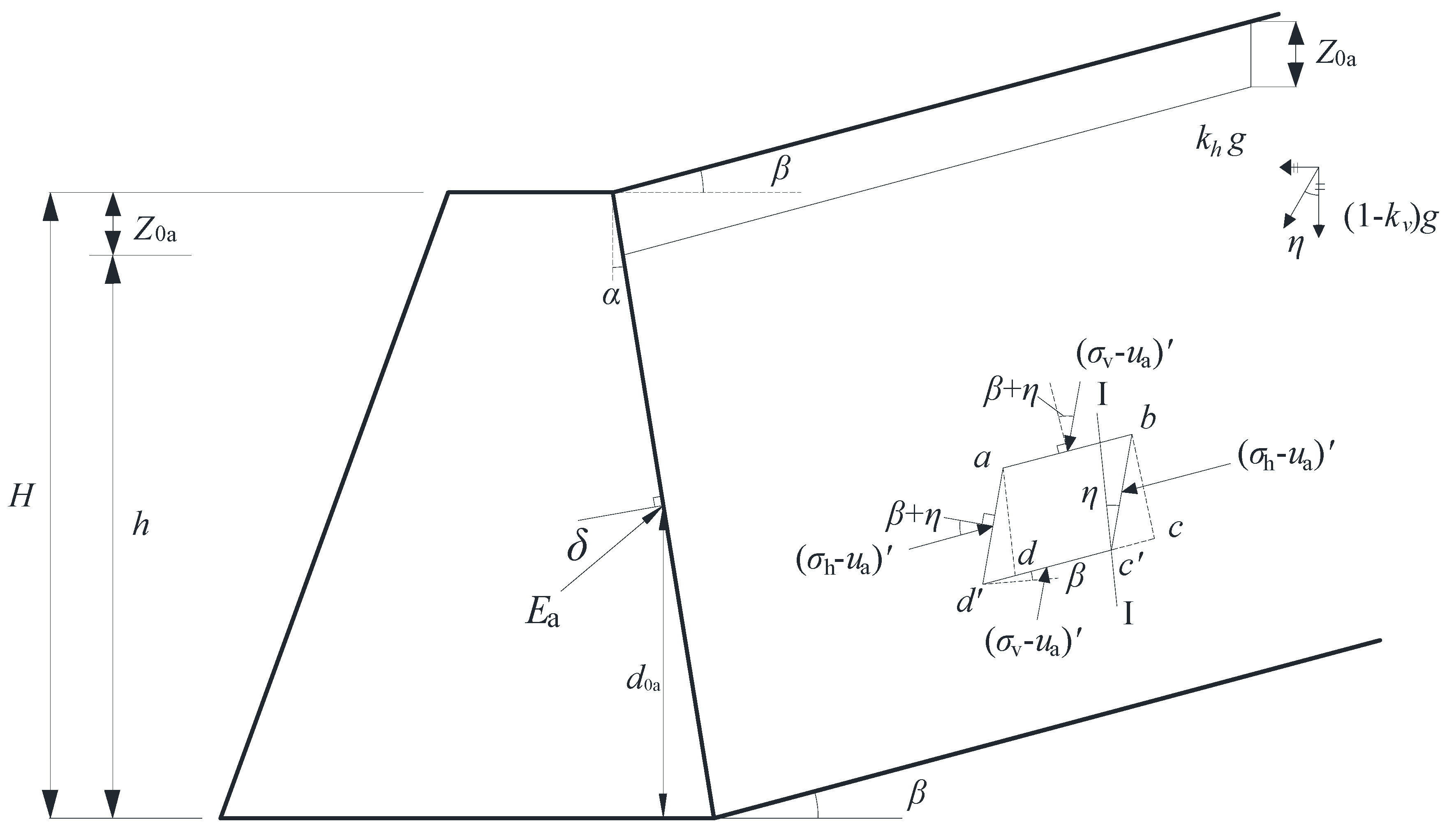
The basic idea of the pseudo-static method is to simplify the seismic action into an inertial force acting on the research object. As shown in Figure 1, H is the wall height, β is the dip angle of the backfill, δ represents the interface friction angle between the retaining wall and the backfill, α is the inclination of the wall back, kh and kv are the horizontal and vertical seismic coefficients, Ea is the resultant force of the active earth pressure, (σv − ua) and (σh − ua) are the net normal stresses, d0a denotes the gravitational distance from the resultant action position to the bottom, and z0a is the crack depth. Assuming the direction of the vertical seismic force to be upward and the direction of the horizontal seismic force to be outward, the seismic angle η could be obtained by
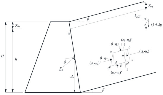
Figure 1.
Calculation model.
Taking a rhombus element (abcd) as the study object, ad and bc are parallel to the wall back, while ab and cd are parallel to the surface of the backfill. During an earthquake, the research element turns into abc′d′, where ad and bc are rotated by seismic angle η and the net normal stress (σv-ua) turns into (σv-ua)′ with an intersection angle of η.
If the pore air in the soil communicates with external atmosphere, ua = 0. Thus, we get
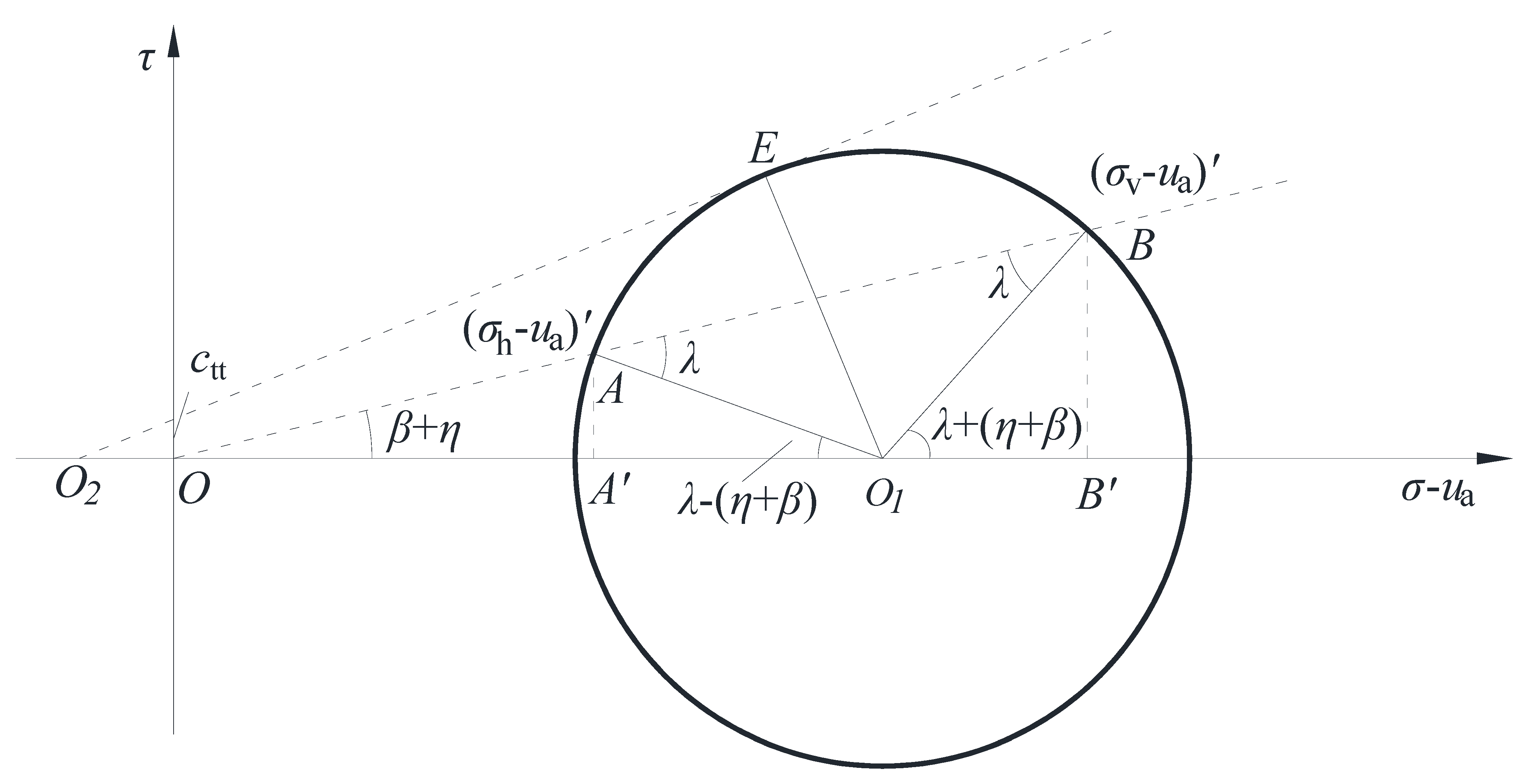
in which γ represents the actual volumetric weight of the backfill, and z is the depth. The stress characteristics of the active limit equilibrium state on the rhombus unit could be presented by the Mohr circle in Figure 2. The process could be stated as follows [20]. (1) Draw a line OB with an intersection angle of η + β from the coordinate origin, and mark B by a length of (σv − ua)′, which is the net stress acting on ab. (2) Determine a Mohr circle O1 with a radius of R through point B, tangent to shear strength envelope O2E. (3) The circle intersects the line OB at the point A, which represents the net stress (σh − ua)′ acting on ad′.
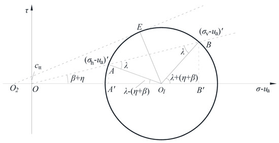
Figure 2.
The Mohr stress circle of rhombic unit.
In the triangle O1EO2,
In triangles O1BB′ and OBB′, following equation could be obtained:
Under the active earth pressure state, (σh − ua)′ could be obtained from Equations (9)–(11):
in which
2.2.2. Intensity of Seismic Active Earth Pressure
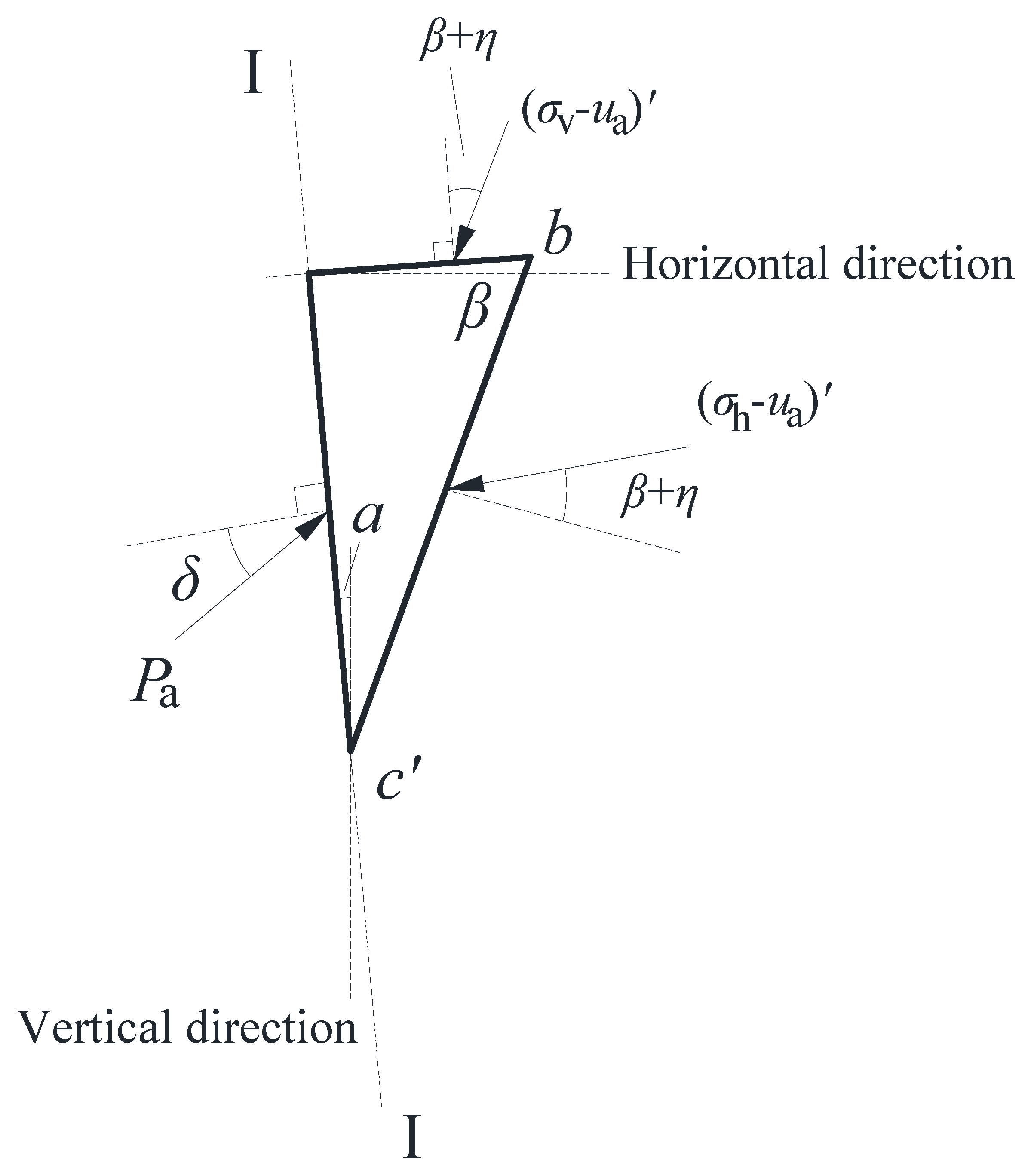
Since the side ad′ is not parallel to the wall back, (σh − ua)′ acting on side ad′ is unequal to the earth pressure intensity pa loading on the wall back. In order to get the active earth pressure intensity, a conversion should be performed, as shown in Figure 3.
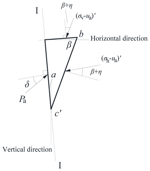
Figure 3.
The stress analysis for the intensity of earth pressure.
According to the mechanical equilibrium state in horizontal direction,
Simplify the above equation and we get
in which the active earth pressure coefficient Ka would be
2.2.3. Resultant Pressure and the Acting Position
Ignoring the tensile strength and supposing pa = 0, the crack depth z0a could be obtained from Equation (17):
The resultant active earth pressure can be calculated by definite integral:
where
Subsequently, the height of the acting position of the resultant pressure could be denoted as
3. Analyses and Results
3.1. Distribution of Seismic Active Earth Pressure
There are several factors with distinct effects involved in the model, including wall height H, inclination of wall back α, the dip angle of backfill β, unit weight γ, effective cohesion c′, effective friction angle φ′, matric suction (ua − uw), matric suction related friction angle φb, interface friction angle δ, vertical seismic coefficient kv, and horizontal seismic coefficient kh. Parametric study was performed with the case of H = 8 m, α = 10°, β = 10°, γ = 18 kN/m3, c′ = 5 kPa, φ′ = 22°, (ua − uw) = 30 kPa, φb = 14°, δ = 10°, kv = 0, kh = 0.1. Without specifications, the residual parameters remain constant when the effect of each parameter is being evaluated.
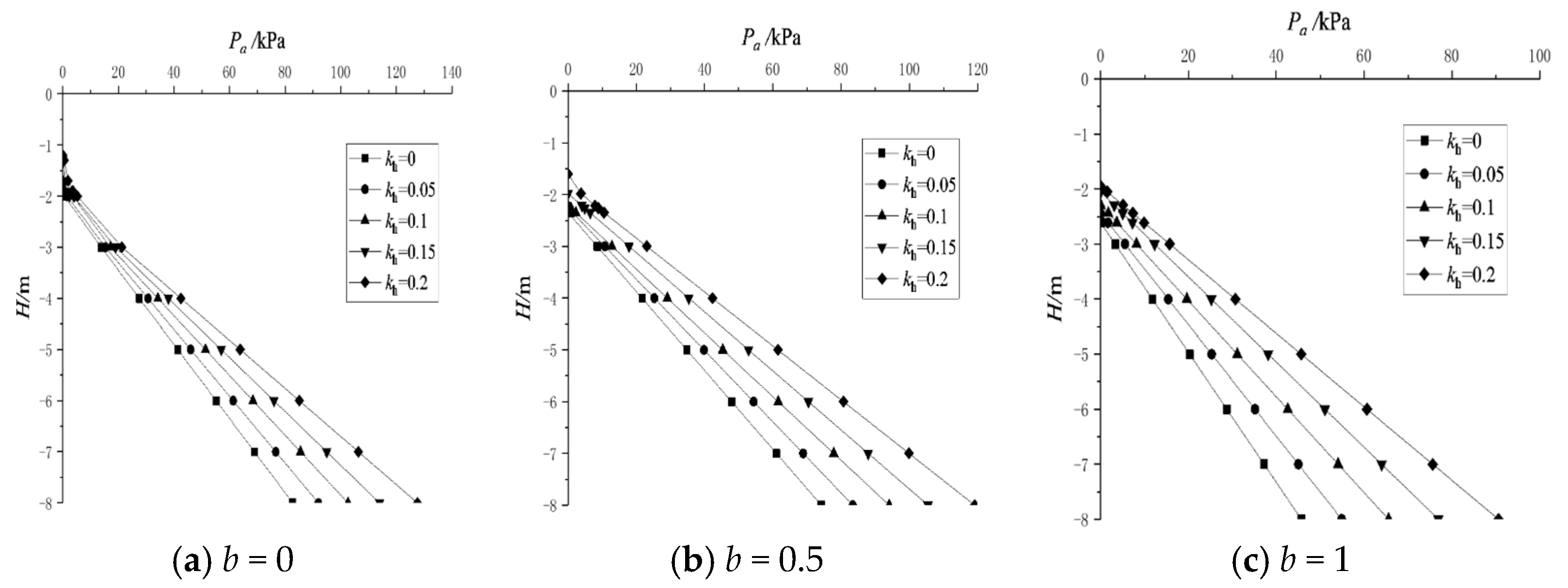
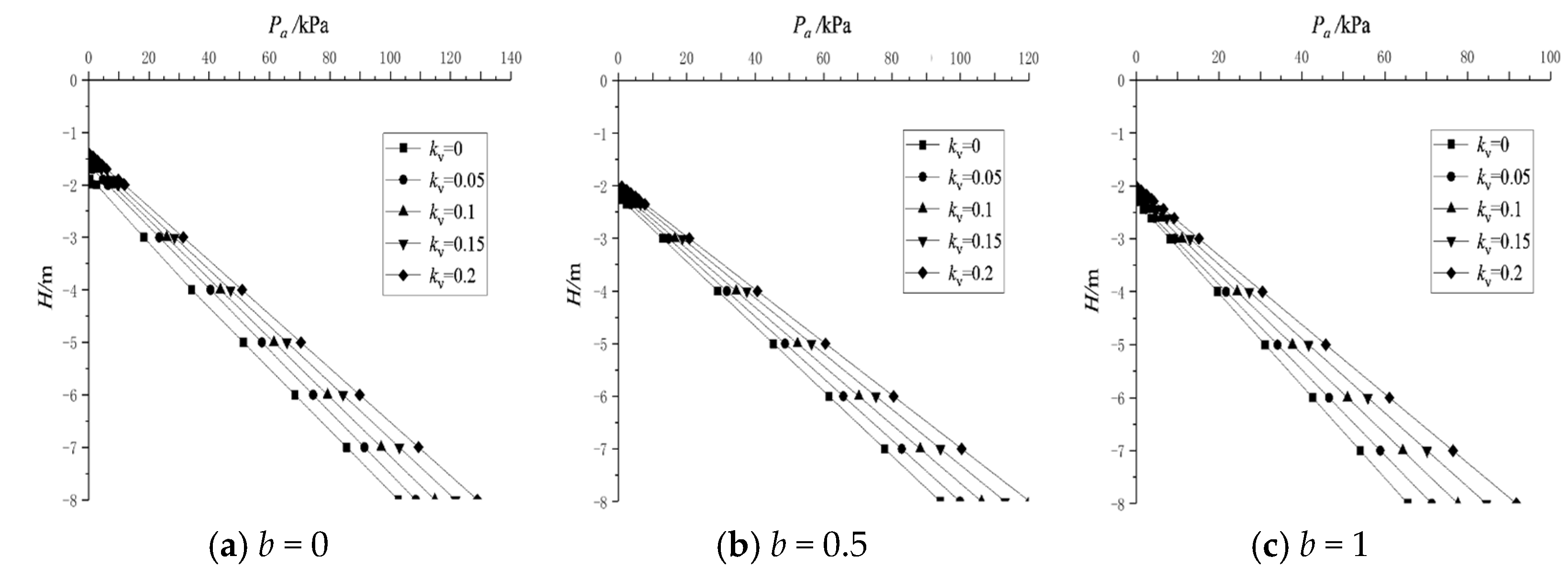
3.1.1. Effect of Seismic Coefficients
(1) From Figure 4 and Figure 5, it could be recognized that the intensity of Rankine active earth pressure is positively correlated with both seismic coefficients; that is, with the increasing of the seismic coefficients, the intensity of Rankine active earth pressure will enlarge to some extent. For instance, the earth pressure at a 4 m depth with b = 0.5 and kv = 0 increases by 35% when kh increases from 0 to 0.1. In addition, the intensity of Rankine active earth pressure increases near linearly in the depth direction, but the earth pressure intensity within about 2 meters of depth seems inconspicuous due to the existence of soil cohesion.
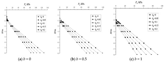
Figure 4.
Intensity distribution of Rankine active earth pressure (kv = 0).
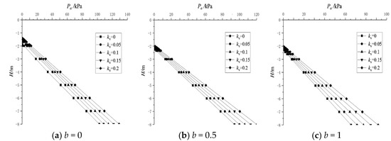
Figure 5.
Intensity distribution of Rankine active earth pressure (kh = 0.1).
(2) Figure 4 and Figure 5 indicate that with the decrease of the seismic coefficients or increase of the unified strength factor, the acting scope of Rankine active earth pressure moves downward slightly, and the intensity reduces. For instance, the earth pressure at 4 m depth with kh = 0.1, kv = 0.1 decreases by 44% when b increased from 0 to 1.
3.1.2. Effect of Unsaturation Parameters
(1) Table 1 and Table 2 show that the intensity of Rankine active earth pressure increases along the wall back downwardly. The existence of matric suction as well as the attributed friction angle results in shrinkage of the intensity of Rankine earth pressure. On the other hand, the range of “zero intensity” amplifies. Given b = 0.5, the earth pressure at a depth of 4 m reduces from 44.75 kPa to 0 kPa when the matric suction increases from 0 kPa to 90 kPa, and the depth of zero intensity increases to be deeper than 4 m.

Table 1.
Intensity values of Rankine active earth pressure and matric suctions.
Table 2.
Intensity values of Rankine active earth pressure and matric suction related friction angles.
(2) The increment of the unified strength factor also leads to the decrease of the intensity of Rankine active earth pressure. For instance, in the case of φb = 16°, the intensity acting on 4 m of depth reduces from 39.59 kPa (b = 0) to 21.94 kPa (b = 1).
3.2. Resultant Location of Seismic Active Earth Pressure
3.2.1. Effect of Seismic Coefficients
Table 3 indicates that the resultant location rises as seismic coefficients increase, which means the retaining wall would be easier to overturn under earthquakes. Without the consideration of intermediate principal stress, the resultant location would also be higher. At the same variation levels of seismic coefficients, the effect of the horizontal seismic coefficient on the resultant point is more significant. For instance, in the case of kh = 0.1 and b = 1, the resultant point of earth pressure varies from 2.20 m to 2.31 m when kv increases from 0 to 0.2. Comparatively, for kv = 0.1 and b = 1, the resultant point moves from 2.08 m to 2.38 m when kh increases from 0 to 0.2.
Table 3.
Resultant location of Rankine active earth pressure and seismic coefficients.
3.2.2. Effect of Unsaturation Parameters
Table 4 shows that the resultant location moves down as the matric suction or matric-suction-attributed friction angle become larger. The intermediate principal stress causes a reduction of resultant acting height, as well. In the case of (ua−uw) = 30 kPa and φb = 14°, the resultant point moves downwardly from 2.43 m to 2.02 m when the intermediate principal stress is fully considered. It could be inferred that the unsaturation characteristics and intermediate principal stress would be beneficial to the anti-overturning stability.
Table 4.
Resultant location of Rankine active earth pressure and unsaturation parameters.
3.3. Verification
3.3.1. Comparison with Classic Rankine Solution
In order to compare with the classic Rankine theory, when re-writing Equations (14), (15) and (18) with the setting of α = β = δ = η = φb = (ua−uw) = kv = kh = b = 0 we get
It could be seen that Equation (24) is completely consistent with the expression of the classical Rankine active earth pressure coefficient by substituting shear strength parameters.
3.3.2. Comparison with Unsated Solution
For unsaturated soils, Zhao’s solution [21] was selected for comparative research. Computing parameters are H = 8m, α = 10°, β = 10°, γ = 18 kN/m3, c′ = 5 kPa, φ′ = 22°, φb = 14°, δ = 10°, kv = 0, kh = 0.1. The results are illustrated in Figure 6.
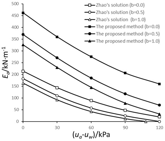
Figure 6.
Comparative research of unsaturated soil.
The proposed method is derived from the Rankine theory, while Ref. [21] presents a unified solution of Coulomb’s active earth pressure. Obviously, the Rankine and Coulomb models would lead to different calculation results. However, both the results showed the same variation regularity or trend of earth pressures. It is shown that active earth pressure is negatively correlated with matric suction, and it will gradually approach zero when the matric suction is high enough. Meanwhile, the difference between these two methods might be mainly due to the earthquake effect. Comparing to the static analysis in Ref. [21], the active earth pressure shows a significant increment when horizontal seismic coefficient kh = 0.1 is taken into consideration, especially when accompanied with low matric suctions. On the other hand, the increase of the unified strength factor will cause a reduction to the earth pressure in practical engineering. Zhao’s solution would be incapable for seismic cases; thus, the application scope is broadened by the proposed method.
3.3.3. Comparison with Seismic Solution
For the seismic state, Zhang’s solution [20] was adopted to compare with the proposed method. Parameters are specified as follows: H = 8, α = 10°, β = 10°, γ = 18 kN/m3, δ = 10°, kv = 0, c′ = 5 kPa, φ′ = 22°, (ua − uw) = 30 kPa, φb = 14°. The Ka − kh curves are presented in Figure 7.
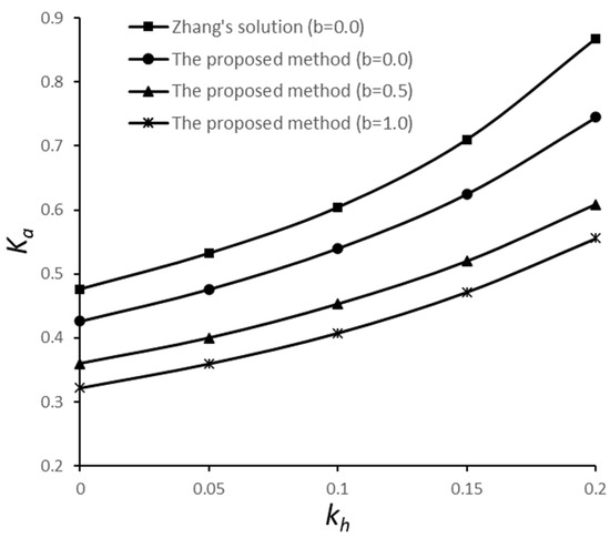
Figure 7.
Comparative research of seismic cases.
In Figure 7, all Ka values grow faster and faster as the horizontal seismic coefficient increases, and the Rankine active earth pressure decreases by about 10% when considering the unsaturation characteristics in the proposed method. Also, the earth pressure reduces as the intermediate principal stress is taken into account. Two methods present the same variation trend of the active earth pressure coefficient for saturated soil; however, Zhang’s solution is not applicable for the unsaturation state. Conclusively, the proposed method has a more extensive application field.
4. Conclusions
- (1)
- By combining the shear strength model of unsaturated soil and the unified strength theory, the calculation model of seismic active earth pressure for unsaturated inclined backfill was deduced. The proposed method could be simplified to those in the previous literature under certain conditions. It extends the application range of the classic Rankine theory by taking earthquake, unsated soil, inclined rough wall back, non-horizontal backfill surface, and the intermediate principal stress into consideration.
- (2)
- As the seismic coefficients increase, the intensity of the Rankine active earth pressure will become larger. The earth pressure at 4 m depth with b = 0.5 and kv = 0 increased by 35% when kh increased from 0 to 0.1. With the decrease of the seismic coefficients or increase of the unified strength factor, the acting scope of Rankine active earth pressure moves downward slightly and the intensity reduces. The earth pressure at 4 m depth with kh = 0.1 and kv = 0.1 decreased by 44% when b increased from 0 to 1.
- (3)
- The horizontal seismic coefficient had a more significant effect on the resultant point location. For instance, in the case of kh = 0.1 and b = 1, the resultant point of earth pressure varied from 2.20 m to 2.31 m when kv increased from 0 to 0.2. Comparatively, for kv = 0.1 and b = 1, the resultant point moved from 2.08 m to 2.38 m when kh increased from 0 to 0.2. The intermediate principal stress caused a reduction of resultant acting height as well. In the case of (ua−uw) = 30 kPa and φb = 14°, the resultant point moved downwardly from 2.43 m to 2.02 m when the intermediate principal stress was taken fully into consideration.
- (4)
- As verification shows, the proposed model and algorithm are fit for seismic or unsaturated conditions. Owing to the scarce examples reported in the research subdivision, the validity of the proposed solution needs to be further examined by more examples. In any case, due to the consideration of the intermediate principal stress in the soil, the calculation result would be closer to the real solution theoretically. However, since it is difficult to determine an objective and accurate value for the unified strength factor (b), the solution is still a certain distance from engineering application, and more comparative research should be performed.
Author Contributions
Conceptualization, W.F.; methodology, W.L.; software, H.S., W.L.; validation, H.S., W.L. and Y.W.; formal analysis, W.L. and H.S.; writing—original draft preparation, H.S., W.L.; writing—review and editing, W.F., H.S. and Y.W.; visualization, H.S. and Y.W.; supervision, W.F.; project administration, W.F.; funding acquisition, W.F. All authors have read and agreed to the published version of the manuscript.
Funding
This research was funded by the Natural Science Foundation, China, grant number: 52178413, and the Natural Science Foundation of Hunan Province, China, grant number: 2022JJ30593.
Data Availability Statement
A part of the raw data cannot be shared at this time, as the data also forms part of an ongoing study.
Conflicts of Interest
The authors declare no conflict of interest.
Abbreviations
| F and F′ | are yield functions under different stress conditions |
| σ | is the total normal stress |
| σ1, σ2 and σ3 | are the principal stresses and σ1 ≥ σ2 ≥ σ3 |
| ua and uw | are the pore air pressure and pore water pressure |
| σt and σc | are the tensile strength and compressive strength of the filling |
| τf | is the shear strength of unsaturated soil |
| c′ and φ′ | are the effective cohesion and effective friction angle of the saturated soil |
| φb | is the friction angle attributed by the matric suction |
| c′t and φ′t | are unified effective cohesion and unified effective friction angle |
| φbt | is the unified friction angle attributed by the matric suction |
| b | is the unified strength factor (0 ≤ b ≤ 1) |
| ctt | is the apparent cohesion |
| H | is the wall height |
| β | is the dip angle of backfill |
| δ | is the interface friction angle between the retaining wall and the backfill |
| α | is the inclination of wall back |
| kh and kv | are horizontal and vertical seismic coefficients |
| Ea | is the resultant force of the active earth pressure |
| pa | is the earth pressure intensity |
| Ka | is the active earth pressure coefficient |
| (σv−ua) and (σh−ua) | are the net normal stresses acting in different direction |
| d0a | is the gravitational distance from the resultant action position to the bottom |
| z0a | is the crack depth |
| η | is the seismic angle |
| γ | is the volumetric weight of the backfill |
References
- Hu, H.; Yang, M.; Lin, P.; Lin, X. Passive Earth Pressures on Retaining Walls for Pit-in-Pit Excavations. IEEE Access 2018, 7, 5918–5931. [Google Scholar] [CrossRef]
- Wang, Z.Y.; Liu, X.X.; Wang, W.W. Calculation of nonlimit active earth pressure against rigid retaining wall rotating about base. Appl. Sci. 2022, 12, 9638. [Google Scholar] [CrossRef]
- Pufahl, D.E.; Fredlund, D.G.; Rahardjo, H. Lateral earth pressures in expansive clay soils. Can. Geotech. J. 1983, 5, 134–146. [Google Scholar] [CrossRef]
- Fu, D.; Yang, M.; Deng, B.; Gong, H. Estimation of active earth pressure for narrow unsaturated backfills considering soil arching effect and interlayer shear stress. Sustainability 2022, 14, 12699. [Google Scholar] [CrossRef]
- Ren, C.J.; Jia, H.B. The influence of Unsaturated Soil’s Characteristics on Rankine Earth Pressure. Sci. Technol. Eng. 2015, 15, 78–82. [Google Scholar]
- Yao, P.F.; Zhang, M.; Dai, R. Generic Rankine theory for unsaturated soils. J. Eng. Geol. 2004, 12, 285–291. [Google Scholar]
- Zhang, C.G.; Zhao, J.H.; Zhang, D.F. Nonlinearity of unsaturated soils strength and its influence on passive earth pressure. Journal of Guangxi University: Nat. Sci. Ed. 2012, 37, 797–802. [Google Scholar]
- Wang, D.J.; Tong, L.Y.; Qiu, Y.F. Rankine’s earth pressure analysis of unsaturated soil under condition of rainfall infiltration. Rock Soil Mech. 2013, 34, 3192–3194. [Google Scholar]
- Zhang, J.; Hu, R.L.; Yu, W.L. Sensitivity analysis of parameters of Rankine’s earth pressure with inclined surface considering intermediate principal stress. Chin. J. Geotech. Eng. 2010, 32, 1566–1572. [Google Scholar]
- Zhao, J.H.; Yin, J.; Zhang, C.G. Unified solutions of Rankine’s earth pressure of unsaturated soil under rainfall. J. Archit. Civ. Eng. 2016, 33, 1–6. [Google Scholar]
- Zhang, C.G.; Zhang, Q.H.; Zhao, J.H. Unified solutions of shear strength and earth pressure for unsaturated soils. Rock Soil Mech. 2010, 31, 1871–1876. [Google Scholar]
- Iskander, M.; Omidvar, M.; Elsherif, O. Conjugate stress approach for Rankine seismic active earth pressure in cohesionless soils. J. Geotech. Geoenviron. Eng. 2012, 139, 1205–1210. [Google Scholar] [CrossRef]
- Lin, Y.L.; Yang, G.L.; Zhao, L.H. Horizontal slices analysis method for seismic earth pressure calculation. Rock Soil Mech. 2010, 29, 2581–2591. [Google Scholar]
- Sun, Y. Unified solution of seismic active earth pressure and its distribution on a retaining wall. Rock Soil Mech. 2012, 33, 255–261. [Google Scholar]
- Zhang, G.X. New analysis method of seismic active earth pressure and its distribution on a retaining wall. Rock Soil Mech. 2014, 35, 335–339. [Google Scholar]
- Shi, Y.Q.; Xie, X.L.; Zhang, Q.K.; Jiang, H.; Peng, J.J.; Liao, X. Study on spectrum characteristics of dynamic earth pressure of loess landslides based on wavelet transform. Chin. J. Rock Mech. Eng. 2020, 39, 2570–2581. [Google Scholar]
- Liu, H.; Kong, D.Z.; Gan, W.S.; Wang, B.J. Seismic active earth pressure of limited backfill with curved slip surface considering intermediate principal stresses. Appl. Sci. 2022, 12, 169. [Google Scholar] [CrossRef]
- Bishop, A.W.; Blight, G.E. Some aspects of effective stress in saturated soils. Geotechnique 1963, 13, 177–197. [Google Scholar] [CrossRef]
- Fredlund, D.C.; Morgenstem, N.R.; Widger, R.A. The shear strength of unsaturated soils. Can. Geotech. J. 1978, 15, 313–321. [Google Scholar] [CrossRef]
- Zhang, J.; Wang, X.Z.; Hu, R.L. Analysis of seismic active earth pressure of backfill with infinite inclined surface behind non-vertical retaining wall. Rock Soil Mech. 2017, 38, 1069–1075. [Google Scholar]
- Zhao, J.H.; Liang, W.B.; Zhang, C.G. Unified solutions of Coulomb’s active earth pressure for unsaturated soils. Rock Soil Mech. 2013, 34, 609–615. [Google Scholar]


Disclaimer/Publisher’s Note: The statements, opinions and data contained in all publications are solely those of the individual author(s) and contributor(s) and not of MDPI and/or the editor(s). MDPI and/or the editor(s) disclaim responsibility for any injury to people or property resulting from any ideas, methods, instructions or products referred to in the content. |
© 2023 by the authors. Licensee MDPI, Basel, Switzerland. This article is an open access article distributed under the terms and conditions of the Creative Commons Attribution (CC BY) license (https://creativecommons.org/licenses/by/4.0/).