Abstract
In the field of geotechnical engineering, the problems of liquefaction and land subsidence are of major concern. In order to mitigate or prevent damage from liquefaction, the chemical injection method is actively used as one of the countermeasures for ground improvement. However, a complete understanding of the long-term sustainability of improved grounds is still unavailable due to a lack of knowledge of the influencing parameters. Thus, the chances of chemical injection accidents cannot be ruled out. In this study, the compressive strength of improved grounds by the granulated blast furnace slag (GBFS), one of the grouting materials used in the chemical injection method, was evaluated and used for a time-series prediction of long-term sustainability. The objective of this study was to evaluate the accuracy and validity of the prediction method by comparing the prediction results with the test results. The study was conducted for three different models, namely, the autoregressive integrated moving average (ARIMA) model, the state-space representation (SSR) model, and the machine learning predictive (MLP) model. The MLP model produced the most reliable results for the prediction of long-term data when the input information was sufficient. However, when the input data were scarce, the SSR model produced more reliable results overall. Meanwhile, the ARIMA model generated the highest degree of errors, although it produced the best results compared to the other models depending on the criteria. It is advised that studies should be continued in order to identify the parameters that can affect the long-term sustainability of improved grounds and to simulate various other models to determine the best model to be used in all situations. However, this study can be used as a reference for the selection of the best prediction model for similar patterned input data, in which remarkable changes are observed only at the beginning and become negligible at the end.
1. Introduction
During an earthquake, liquefaction can cause problems such as the tilting of buildings and the lifting of sewer pipes. The main reason behind it is the change in soil behaviors from solid- to fluid-like due to the increase in pore water pressure and the subsequent decrease in effective stress [1]. A change in pore water pressure is concerned with other problems related to ground water level [2]. Many researchers have studied the methods to mitigate the liquefaction problem such as ground improvement using additives [3], ground stabilizing methods [4,5,6,7], etc. Duan et al. [8] studied the state parameters to evaluate the soil liquefaction potential and proposed the group method of data handling (GMDH)-type neural network to estimate the state parameters [9]. On the other hand, Padmanabhan and Shanmugam [10] proposed the installation of sand compaction piles for a better seismic response of the liquefiable sand deposits. Nakao et al. [11] studied the simulation of liquefaction itself so that future designs can be more effectively designed. Meanwhile, the chemical injection has also been actively used as a ground improvement method to combat these adverse effects. The method can increase ground stability by reducing ground permeability and increasing ground strength [12,13]. Askoy [12] reported that chemical injection is an effective method to prevent ground settlement caused by groundwater drainage. Moreover, this method is environmentally friendly as it produces very little industrial waste for almost all types of soils, with very little construction noise or vibrations. In addition to ground stabilization, the chemical injection method has also been used in support anchoring, strata sealing, reducing and diversifying groundwater flow and water ingress, and creating a load-bearing ring during tunneling operations [12]. Despite all these advantages and its popularity in the civil engineering field, there are unfortunately still many unknowns left to be discovered in relation to this method. For example, to confirm the efficiency of this method for ground improvement, reliance must be placed on post-investigations of the improved soil by uniaxial compressive strength tests, because direct visualization technology is still in its infancy. Moreover, depending on the soil type, compression test samples are prone to disturbances during their extraction, which often results in inaccurate interpretations.
A literature review on the subject shows that many studies on the long-term curing of the uniaxial compressive strength of the granulated blast-furnace slag (GBFS) used for soil improvement have used an initial start-up strength for 28 days. Xu et al. [14], Yi et al. [15], and Sun and Yi [16] studied the stabilization of subgrade soils using the granulated blast furnace slag at different proportions and temperatures. These studies were conducted for a period of one year and it was found that the addition of slag increased the overall strength. When more slag was added, it was shown to significantly reduce the risk of sulfate attack, alkali–silica reaction, and chloride penetration [17,18,19,20,21,22]. Some researchers have even suggested that the material chosen for the chemical injection should possess certain properties [23,24,25,26,27,28].
Most studies on the long-term curing of chemicals have been conducted for a period of 6 months or 1 year. Very few have been conducted for more than a year. These studies were mainly based on actual field data or long-term experimental data from the laboratory. Data acquisition from an actual experiment or the field involves a tedious process. In addition, if the process is hindered and the data cannot be acquired, it will be a devastating loss of time and resources. Therefore, in this study, the available time-series long-term sustainability of ultrafine grouting materials used in the chemical injection method was verified. Three different prediction models were studied, and the best-fitting prediction model was determined. Since the scientific society nowadays puts its best effort in the decision-making of uncertain matters by various analysis tools considering sustainability [29,30], the main objective of this study is to obtain useful information for establishing and suggesting a reliable model for time-series predictions of the granulated blast furnace slag. Since the prediction pattern depends upon the adopted model and input data characteristics, the result of this study can be used as a reference for other data with similar patterns.
2. Methodologies
In this study, three different prediction models are discussed. The autoregressive integrated moving average (ARIMA) model is a flexible method that can even describe the behavior of nonstationary and seasonal time series [31]. However, the ARIMA model might be inadequate in certain situations, such as for series describing employment [32,33]. The state-space representation (SSR) model can represent many statistical models in a unified manner, for example, an analysis of variance, regression analysis, normal linear models, generalized linear models (GLM), generalized linear mixed models (GLMM), ARIMA, generalized autoregressive conditional heteroscedasticity models (GARCH), stochastic variance models (SV), etc. [34,35,36,37,38,39,40,41]. The machine learning predictive (MLP) model automatically finds patterns in the data and uses those patterns to make predictions [42,43,44,45]. These three models were analyzed using the R software.
2.1. Autoregressive Integrated Moving Average (ARIMA) Model
The general equation of the AR (the p-th order of autoregressive or number of lags) part of the ARIMA is given by Equation (1).
The general equation of the MA (the q-th order of moving average) part of the ARIMA is given by Equation (2).
For the time series data , the general autoregressive moving average model ARMA (, ) is given by Equation (3).
where , , …, are the response variable at time t, t − 1, …, t − p, respectively; , , …, and , , …, are the coefficients to be estimated for Equations (1) and (2) respectively; is the error at any time ; , , …, are the errors in the previous time periods that are incorporated into ; and is the mean.
Assuming as the lag operator (difference) of two consecutive response variables, the number of difference d is carried until the series becomes stationary, and hence, the d-th difference is given by . Therefore, the general equation for the ARIMA model (, , ) is given by Equation (4).
Figure 1 shows the basic flowchart for the working principle of the ARIMA model.
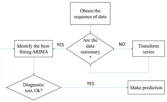
Figure 1.
Flowchart of the autoregressive integrated moving average (ARIMA) model [41].
2.2. State-Space Representation (SSR) Model
The SSR model introduces an unobserved latent random variable x, which is called state, and uses the state to explain the observed value y. By using the SSR model, non-stationary data can be handled. The SSR model is a very flexible statistical model [34,35,36,37,38,39,40] that can create a combination of various statistical models without major restrictions. In this model, “iter” specifies the number of iterations in the given data, whereas “chains” specifies the number of times the “iter” simulation is performed. The SSR model contains two variables, namely, the state and the observed value. When the time-series data are stationary, the value observed at time is generated from the state . The state is then determined only by the state . The values can be expressed by Equations (5) and (6). Equations (3) and (4) are known as the state equation and the observation equation, respectively [39,40].
where is the state value at any time , is the observed value at any time , is the process error at time , and is the observation error in the state.
Figure 2 presents the schematic representation of the SSR model. If the state is stationary, then the difference between the state at time t and the state at time is expected to follow a normal distribution with a zero mean and a standard deviation of . By repeating the same process, the reliability of the results can be checked. In this model, “chains” is specified four times and “iter” is predicted 2000 times.
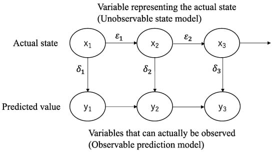
Figure 2.
State-space representation (SSR) model.
2.3. Machine Learning Predictive (MLP) Model
Machine learning is a technique or method for predicting what data will come next by following a set procedure [42,43,44,45]. Figure 3 shows the working steps for the machine learning predictive (MLP) model. The basic steps of the model are as follows: learning the overall picture of machine learning, learning the individual methods, learning how to evaluate the predictions, and trying to use machine learning for specific tasks. The machine learning method in this study employed the support vector machine (SVM). The SVM [45,46,47,48,49] is a two-class classification machine learning method with supervised learning. Supervised learning is a type of machine learning method in which the machine is given a problem with an associated answer and learns them by adjusting the parameters in the program so that the answer calculated by the program is similar to the prepared answer.
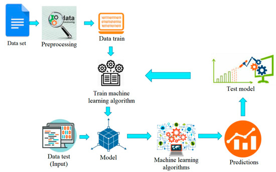
Figure 3.
Working steps of the machine learning predictive (MLP) model.
The SVMs can handle a variety of problems using two methods, namely, the kernel method (the data on a plane can be divided not only by straight lines, but also by curves for various problems) and the margin maximization method (the margin is the region bounded by two hyperplanes that linearly separate two data, and the maximum-margin hyperplane is the hyperplane that lies halfway between them), both of which can be used to determine a straight line that will successfully divide the input data.
For the hard margin, is minimized and subjected to Equation (7).
where represents the hyperplane for a dataset of n points (), …, (), is the normal vector of the hyperplane, determines the offset of the hyperplane from the origin along the normal vector, and the superscript denotes the conjugate transpose.
For the soft margin, Equation (8) is minimized.
where the parameter determines the trade-off between increasing the margin size and ensuring that lies on the correct side of the margin.
In summary, the support vector machine (SVM) is a machine learning model that is capable of learning the fluctuation patterns of the input data, and when it recognizes patterns of the up and down values in the data, it can construct a machine learning model to predict the next movement.
3. Results and Discussion
3.1. Uniaxial Compression Strength of the Improved Body
Figure 4 shows the experimental results of the uniaxial compressive strength with respect to the time for the improved body in a 10-year period, with the GBFS being injected. The data were obtained from long-term curing experiment results for various grouting materials. Several samples were prepared for each batch of the GBFS injected curing test and the mean strength of the samples at a particular interval of measurement was adopted as the strength of that period. The data were used as the benchmark to determine the precision of each method by comparing the difference between the predicted results and the benchmark data. The data were recorded six times in the first year where the initial strength gain of the samples was rapid. After that, the data was recorded over 2 years except for the 10-year data. It can be seen in the figure that in the initial 28 days, approximately 85% of the total strength is gained, reaching the value of 3.1 N/mm2. Then, the gain in strength becomes negligible and the maximum strength of 3.79 N/mm2 is reached in a year. The data show a decrease in strength during the following 5-year period, after which the strength starts to increase again, reaching a final strength of 3.73 N/mm2 at the end of 10 years.
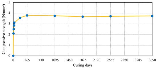
Figure 4.
Time-series compressive strength of the granulated blast-furnace slag (GBFS).
3.2. Prediction Results from the ARIMA Model
Figure 5 shows the prediction results from the ARIMA model after the model fitting shown in Figure 6. In total, there were 21 models and the best-fitting model was the ARIMA (4, 2, 1). The simulation was completed for four different sets of data, namely, 28 days, 180 days, 1 year, and 5 years. It can be confirmed from Figure 5 that the prediction results for short periods comprised single values, but after certain periods, the prediction results fell in a range of values. In other words, for the 28-day sets of input data, the prediction results comprised single values for approximately 283 days. Similarly, for the 180-day, 1-year, and 5-year sets of input data, the results comprised single values for approximately 452, 388, and 2081 days, respectively. After that, however, the obtained results fell in a range of values showing the maximum and minimum strength the concrete can gain during those periods. The predicted maximum strength was very high. When compared with the actual experimental data, the value is considered incorrect. The minimum value for each prediction was zero as it is theoretically impossible to obtain a value below zero. The predicted results, when compared with the actual experimental data, produced accurate results for the 1-year and 5-year sets of input data with the single-value output. Meanwhile, the output results were lower than the actual experimental data for the 28-day and 180-day sets of input data in the part of the single-value output. The main reason for this discrepancy might be the limited amount of input data and the working principle of this method. As for the range of values, it diverged exponentially from the actual experimental data. Thus, it cannot be used as a reliable reference for long-term prediction. However, since the immediate prediction results for all four models were accurate for a short span and the accuracy span increased proportionately for a large amount of input data, the applicability of the ARIMA model for long-term prediction might be limited.
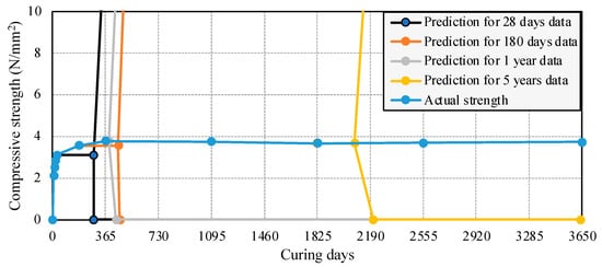
Figure 5.
Prediction results of the ARIMA model.
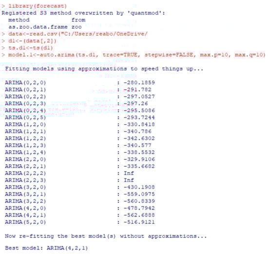
Figure 6.
Fitting results of the ARIMA model.
3.3. Prediction Results by SSR Model
Figure 7 shows the prediction results by the SSR model for the input data of the experimental compression strength of the GBFS. A simulation was conducted for the sets of input data for 28 days, 180 days, 1 year, and 5 years, respectively, and a prediction was made for the 10-year time period in each simulation. In this model, the results were outputted in the form of maximum and minimum values and when compared with the actual strength, the actual strength was found between the predicted values for all cases, which verified the correctness of the prediction. The 5-year input data produced the most accurate results, suggesting a correlation between the amount of input data and accuracy. However, it can be observed that the prediction results for the 28-day input data were more accurate than those of the 180-day and 1-year input data. The reason for this is the detailed settings of “iter” and “chains”. In the model, “iter” specifies the number of iterations in the given data, and “chains” specifies the number of times the simulation is performed using “iter”. The predictions are made by estimating the data change in which the state changes and observation errors are distinguished. This can also be observed in the results when the prediction results become more accurate for more input data where the data change pattern has been stabilized. The state is obtained after adding the process error to the predicted value used in the previous time. Then, the observed value is obtained by adding the observation error to the state. These observation and process errors control the “iter” and “chains”. The actual experimental data pattern changed remarkably compared to the initial trend of the 28-day data, causing the prediction results to deviate from the actual results.
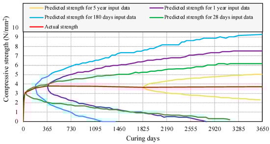
Figure 7.
SSR model results for different input data.
3.4. Prediction Results by MLP Model
Figure 8 and Figure 9 show the prediction results by the MLP model for the 1-year and 10-year periods, respectively. The predictions were made for 1 year and 10 years using the 180-day and 5-year sets of input data, respectively. The model can only make reliable predictions for periods equivalent to the amount of input data, i.e., for the 10-year prediction, 5 years of input data were required, and for the 1-year prediction, 180 days of input data were required. The predicted strength was 4.34 N/mm2 for 1 year and 3.73 N/mm2 for 10 years. In both cases, the results were predicted for the input data with and without omission of the highly fluctuating 0–28-day data. The reason for this is to obtain results closer to those of the actual experiments. As can be confirmed in Figure 8 and Figure 9, the predicted results for 0–28 days included data-produced results that deviated from the actual results in the initial phase. The reason for this is that the method learns the input data, recognizes the patterns of fluctuations for all the data, and determines the balanced prediction results. If the highly fluctuating part is omitted in the input phase, then its influence on the predicted results will decrease. However, omitting the highly fluctuating part will result in lower predicted results than the actual compressive strength after a certain period. Meanwhile, the results in Figure 8 were observed to be the best fitting to the actual data, with a very small deviation even when the 0–28 days data were included. This is due to the higher amount of input data, and likewise in other models, proportional to the amount of input data. Therefore, the influence of the initial fluctuating part became less. The model was found better than other methods, suggesting that the MLP might be the best prediction model for this study. This study used actual data to compare with predicted results so that the best model can be selected. However, if the actual data are not available, then, based on the trend in the predicted data, the data obtained by omitting the highly fluctuating input data appear more reliable and accurate.
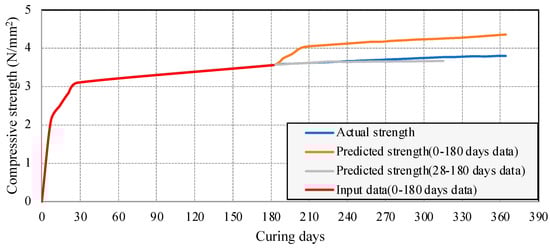
Figure 8.
MLP model results for 1 year using the 180-day input data.
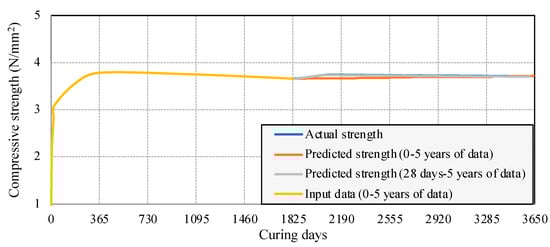
Figure 9.
MLP model results for 10 years using the 5-year input data.
3.5. Comparison between the Three Different Models
Figure 10 and Figure 11 show comparisons of the prediction results between the ARIMA model, the SSR model, and the MLP model for the 180-day and 5-year input data, respectively. Among the three models, the most accurate model was found to be the MLP model, whereas the least accurate model was the ARIMA model in terms of the overall results. However, it can also be observed from Figure 11 that the predicted data for the ARIMA has single values for short periods, except for the 180-day input data. During this period, the output results for the ARIMA model were more accurate than those of the MLP model. Thus, depending on the requirements, the best model could be any of the three models.
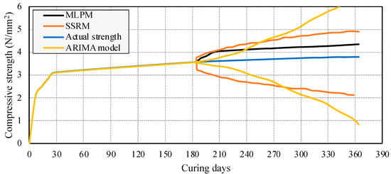
Figure 10.
Comparison among three models for 180-day input data.
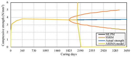
Figure 11.
Comparison of the three models for the 5-year input data.
4. Conclusions and Future Studies
It can be concluded that the MLP model is the most accurate prediction model compared to the ARIMA model and the SSR model. The accuracy of the output results of the MLP model further increased when the highly fluctuating data were omitted from the input data. For all three methods, their accuracy increased as the input data volume increased. Since the ARIMA model generated very large amount of overall errors when making long-term predictions from a minimum amount of input data, the results cannot be used for future reference. The followings are the major conclusions drawn from this study.
- (1)
- The output results of the SSR model were moderate at their best. The accuracy increased with the increase in the amount of input data amount, although the output results were still generated in a range instead of a single value. However, the 10-year period prediction from 28 days of data was found to be more accurate than that from the 180 days and 1-year input data.
- (2)
- Although the MLP model generated the smallest errors among the three models, the margin of error remained and was only omitted when the highly fluctuating data were omitted from the input data. This might bring some sort of conflict in the scientific community regarding its reliability.
- (3)
- Since the MLP model can generate reliable results only for equivalent input data, the SSR model might be a better choice for long-term forecasting with a small amount of input data. In addition, since the chances of availability of long-term data, such as 5-year period data, are very low in all cases, the MLP method might not be favored in all situations.
- (4)
- The ARIMA model produced the most accurate predictions for short periods when the amount of input data was large, such as the case of 5-year input data, where the results for 730 days were more accurate than those using the MLP model.
All three models have shown some shortcomings in terms of achieving the most reliable outcome, and, therefore, it is difficult to claim any one of these models is absolutely the best model for all situations. If the amount of available input data is equivalent to the future prediction period, then the MLP model is the best choice. If the amount of input data is small, but the prediction period is long-term, the SSR model is the best option. However, if the amount of available input data is large and the prediction period is short, then the ARIMA model is the best option. Thus, it is suggested that future research can be conducted with more time-series prediction models and comparisons should be made among these models to yield better results.
Author Contributions
Conceptualization, S.I. and S.N.; methodology, S.I.; software, S.S.; validation, S.S. and C.C.; formal analysis, S.S. and C.C.; investigation, H.K.; resources, H.K.; data curation, S.S. and C.C.; writing—original draft preparation, S.S.; writing—review and editing, S.I. and S.N.; visualization, S.I.; supervision, S.I.; project administration, S.I.; funding acquisition, S.I. and H.K. All authors have read and agreed to the published version of the manuscript.
Funding
This research received no external funding.
Institutional Review Board Statement
Not applicable.
Informed Consent Statement
Not applicable.
Data Availability Statement
Data is contained within the article.
Conflicts of Interest
The authors declare no conflict of interest.
References
- Sharma, M.; Satyam, N.; Reddy, K.R. State of the art review of emerging and biogeotechnical methods for liquefaction mitigation in sands. J. Hazard. Toxic Radioact. Waste 2021, 25, 03120002. [Google Scholar] [CrossRef]
- Intui, S.; Inazumi, S.; Soralump, S. Sustainability of soil/ground environment under changes in groundwater level in Bangkok plain, Thailand. Sustainability 2022, 14, 10908. [Google Scholar] [CrossRef]
- Inazumi, S.; Hashimoto, R.; Shinsaka, T.; Nontananandh, S.; Chaiprakaikeow, S. Applicability of additives for ground improvement utilizing fine powder of waste glass. Materials 2021, 14, 5169. [Google Scholar] [CrossRef]
- Shakya, S.; Inazumi, S.; Nontananandh, S. Potential of computer-aided engineering in the design of ground improvement technologies. Appl. Sci. 2022, 12, 9675. [Google Scholar] [CrossRef]
- Nontananandh, S.; Kuwahara, S.; Shishido, K.; Inazumi, S. Influence of perforated soils on installation of new piles. Appl. Sci. 2022, 12, 7712. [Google Scholar] [CrossRef]
- Inazumi, S.; Kuwahara, S.; Nontananandh, S.; Jotisankasa, A.; Chaiprakaikeow, S. Numerical analysis for ground subsidence caused by extraction holes of removed piles. Appl. Sci. 2022, 12, 5481. [Google Scholar] [CrossRef]
- Nakao, K.; Inazumi, S.; Takaue, T.; Tanaka, S.; Shinoi, T. Evaluation of discharging surplus soils for relative stirred deep mixing methods by MPS-CAE analysis. Sustainability 2022, 14, 58. [Google Scholar] [CrossRef]
- Duan, W.; Congress, S.S.C.; Cai, G.; Liu, S.; Dong, X.; Chen, R.; Liu, X. A hybrid GMDH neural network and logistic regression framework for state parameter–based liquefaction evaluation. Can. Geotech. J. 2021, 99, 1801–1811. [Google Scholar] [CrossRef]
- Duan, W.; Congress, S.S.C.; Cai, G.; Zhao, Z.; Liu, S.; Dong, X.; Chen, R.; Qiao, H. Prediction of in situ state parameter of sandy deposits from CPT measurements using optimized GMDH-type neural networks. Acta Geotech. 2022, 17, 4515–4535. [Google Scholar] [CrossRef]
- Padmanabhan, G.; Shanmugam, G.K. Liquefaction and reliquefaction resistance of saturated sand deposits treated with sand compaction piles. Bull. Earthq. Eng. 2021, 19, 4235–4259. [Google Scholar] [CrossRef]
- Nakao, K.; Inazumi, S.; Takahashi, T.; Nontananandh, S. Numerical simulation of the liquefaction phenomenon by MPSM-DEM coupled CAES. Sustainability 2022, 14, 7517. [Google Scholar] [CrossRef]
- Aksoy, C.O. Chemical injection application at tunnel service shaft to prevent ground settlement induced by groundwater drainage: A case study. Int. J. Rock Mech. Min. Sci. 2008, 45, 376–383. [Google Scholar] [CrossRef]
- Pogaku, R.; Mohd, F.N.H.; Sakar, S.; Cha, Z.W.; Musa, N.; Awang, T.D.N.A.; Morris, L.O. Polymer flooding and its combinations with other chemical injection methods in enhanced oil recovery. Polym. Bull. 2018, 75, 1753–1774. [Google Scholar] [CrossRef]
- Xu, B.; Yi, Y. Soft clay stabilization using ladle slag-ground granulated blast furnace slag blend. Appl. Clay Sci. 2019, 178, 105136. [Google Scholar] [CrossRef]
- Yi, Y.; Li, C.; Liu, S. Alkali-activated ground-granulated blast furnace slag for stabilization of marine soft clay. J. Mater. Civ. Eng. 2015, 27, 04014146. [Google Scholar] [CrossRef]
- Sun, X.; Yi, Y. Utilization of incineration bottom ash, waste marine clay, and ground granulated blast-furnace slag as a construction material. Resour. Conserv. Recycl. 2022, 182, 106292. [Google Scholar] [CrossRef]
- Güneyisi, E.; Gesoğlu, M. A study on durability properties of high-performance concretes incorporating high replacement levels of slag. Mater. Struct. 2008, 41, 479–493. [Google Scholar] [CrossRef]
- Hadj-sadok, A.; Kenai, S.; Courard, L.; Darimont, A. Microstructure and durability of mortars modified with medium active blast furnace slag. Constr. Build. Mater. 2011, 25, 1018–1025. [Google Scholar] [CrossRef]
- Nazari, A.; Riahi, S. RETRACTED: Splitting tensile strength of concrete using ground granulated blast furnace slag and SiO2 nanoparticles as binder. Energy Build. 2011, 43, 864–872. [Google Scholar] [CrossRef]
- Shi, X.; Yang, Z.; Liu, Y.; Cross, D. Strength and corrosion properties of portland cement mortar and concrete with mineral admixtures. Constr. Build. Mate Rials 2011, 25, 3245–3256. [Google Scholar] [CrossRef]
- Shi, X.; Xie, N.; Fortune, K.; Gong, J. Durability of steel reinforced concrete in chloride environments: An overview. Constr. Build. Mater. 2012, 30, 125–138. [Google Scholar] [CrossRef]
- Teng, S.; Lim, T.Y.D.; Sabet, D.B. Durability and mechanical properties of high strength concrete incorporating ultra-fine ground granulated blast-furnace slag. Constr. Build. Mater. 2013, 40, 875–881. [Google Scholar] [CrossRef]
- Song, B.; Zhang, S.; Zhang, D.; Fan, G.; Yu, W.; Zhao, Q.; Liang, S. Inorganic cement grouting for reinforcing triangular zone of highly gassy coal face with large mining height. Energies 2018, 11, 2549. [Google Scholar] [CrossRef]
- Atangana, N.P.G.; Shen, J.S.; Modoni, G.; Arulrajah, A. Recent advances in hori-zontal jet grouting (HJG): An overview. Arab. J. Sci. Eng. 2018, 43, 1543–1560. [Google Scholar] [CrossRef]
- Qiu, J.; Liu, H.; Lai, J.; Lai, H.; Chen, J.; Wang, K. Investigating the long-term settlement of a tunnel built over improved loessial foundation soil using jet grouting technique. J. Perform. Constr. Facil. 2018, 32, 04018066. [Google Scholar] [CrossRef]
- Hwang, J.H.; Lu, C.C. A semi-analytical method for analyzing the tunnel water inflow. Tunn. Undergr. Space Technol. 2007, 22, 39–46. [Google Scholar] [CrossRef]
- Jacob, C.E.; Lohmann, S.W. Non steady flow to a well of constant drawdown in an extensive aquifer. Trans. Am. Geophys. Union 1952, 33, 559–569. [Google Scholar] [CrossRef]
- Kazemian, S.; Huat, B.B.; Arun, P.; Barghchi, M. A review of stabilization of soft soils by injection of chemical grouting. Aust. J. Basic Appl. Sci. 2010, 4, 5862–5868. [Google Scholar]
- Chandra, M.; Shahab, F.; Kek, V.; Rajak, S. Selection for additive manufacturing using hybrid MCDM technique considering sustainable concepts. Rapid Prototyp. J. 2022, 28, 1297–1311. [Google Scholar] [CrossRef]
- Khorsani, M.; Loy, J.; Ghasemi, A.H.; Sharabian, E.; Leary, M.; Mirafzal, H.; Cochrane, P.; Rolfe, B.; Gibson, I. A review of Industry 4.0 and additive manufacturing synergy. Rapid Prototyp. J. 2022, 28, 1462–1475. [Google Scholar] [CrossRef]
- Chatfield, C. The Analysis of Time Series: An Introduction, 6th ed.; Chapman and Hall/CRC: London, UK, 2003. [Google Scholar] [CrossRef]
- Aladağ, E. Forecasting of particulate matter with a hybrid ARIMA model based on wavelet transformation and seasonal adjustment. Urban Clim. 2021, 39, 100930. [Google Scholar] [CrossRef]
- McElroy, T. Finite sample revision variances for ARIMA model-based signal extraction. J. Off. Stat. 2008, 24, 451–467. [Google Scholar]
- Durbin, J.; Koopman, S.J. Time Series Analysis by State Space Methods, 2nd ed.; Oxford Statistical Science Series 38; Oxford University Press: Oxford, UK, 2012. [Google Scholar]
- Duan, L.; Huang, M.; Zhang, L. Use of a state-space approach to predict soil water storage at the hillslope scale on the Loess Plateau, China. CATENA 2016, 137, 563–571. [Google Scholar] [CrossRef]
- Wendroth, O.; Reynolds, W.D.; Vieira, S.R.; Reichardt, K.; Wirth, S. Chapter 11 Statistical approaches to the analysis of soil quality data. Dev. Soil Sci. 1997, 25, 247–276. [Google Scholar] [CrossRef]
- Georgakakos, A.P.; Georgakakos, K.P.; Baltas, E.A. A state-space model for hy-drologic river routing. Water Resour. Res. 1990, 26, 827–838. [Google Scholar] [CrossRef]
- Chiheb, S.; Kherif, O.; Teguar, M.; Mekhaldi, A.; Harid, N. Transient behaviour of grounding electrodes in uniform and in vertically stratified soil using state space rep-resentation. IET Sci. Meas. Technol. 2018, 12, 427–435. [Google Scholar] [CrossRef]
- Hagiwara, J. Time Series Analysis for the State-Space Model with R/Stan; Springer: Singapore, 2021. [Google Scholar] [CrossRef]
- Brockwell, P.J.; Davis, R.A. Introduction to Time Series and Forecasting; Springer: Berlin/Heidelberg, Germany, 2002. [Google Scholar] [CrossRef]
- Dai, J.; Chen, S. The application of ARIMA model in forecasting population data. J. Phys. Conf. Ser. 2019, 1324, 012100. [Google Scholar] [CrossRef]
- Jordan, M.I.; Mitchell, T.M. Machine learning: Trends, perspectives, and prospects. Science 2015, 349, 255–260. [Google Scholar] [CrossRef]
- Butler, K.T.; Davies, D.W.; Cartwright, H.; Isayev, O.; Walsh, A. Machine learning for molecular and materials science. Nature 2018, 559, 547–555. [Google Scholar] [CrossRef]
- Puri, N.; Prasad, H.D.; Jain, A. Prediction of geotechnical parameters using ma-chine learning techniques. Procedia Comput. Sci. 2018, 125, 509–517. [Google Scholar] [CrossRef]
- Inazumi, S.; Intui, S.; Jotisankasa, A.; Chaiprakaikeow, S.; Kojima, K. Artificial intelligence system for supporting soil classification. Results Eng. 2020, 8, 100188. [Google Scholar] [CrossRef]
- Abe, S. Introduction of support vector machines for pattern classification—VI: Current topics. Syst. Control Inf. 2009, 53, 205–210. [Google Scholar] [CrossRef]
- Müller, A.C.; Guido, S. Introduction to Machine Learning with Python: A Guide for Data Scientists; O’Reilly Media Inc.: Sebastopol, CA, USA, 2016. [Google Scholar]
- Naganna, S.R.; Deka, P.C. Support vector machine applications in the field of hydrology: A review. Appl. Soft Comput. 2014, 19, 372–386. [Google Scholar] [CrossRef]
- Raschka, S.; Patterson, J.; Nolet, C. Machine learning in Python: Main developments and technology trends in data science, machine learning, and artificial intelligence. Information 2020, 11, 193. [Google Scholar] [CrossRef]


Disclaimer/Publisher’s Note: The statements, opinions and data contained in all publications are solely those of the individual author(s) and contributor(s) and not of MDPI and/or the editor(s). MDPI and/or the editor(s) disclaim responsibility for any injury to people or property resulting from any ideas, methods, instructions or products referred to in the content. |
© 2023 by the authors. Licensee MDPI, Basel, Switzerland. This article is an open access article distributed under the terms and conditions of the Creative Commons Attribution (CC BY) license (https://creativecommons.org/licenses/by/4.0/).