Abstract
Taking smartphone-made videos for photogrammetry is a convenient approach because of the easy image collection process for the object being reconstructed. However, the video may contain a lot of relatively similar frames. Additionally, frames may be of different quality. The primary source of quality variation in the same video is varying motion blur. Splitting the sequence of the frames into chunks and choosing the least motion-blurred frame in every chunk would reduce data redundancy and improve image data quality. Such reduction will lead to faster and more accurate reconstruction of the 3D objects. In this research, we investigated image quality evaluation in the case of human 3D head modeling. Suppose a head modeling workflow already uses a convolutional neural network for the head detection task in order to remove non-static background. In that case, features from the neural network may be reused for the quality evaluation of the same image. We proposed a motion blur evaluation method based on the LightGBM ranker model. The method was evaluated and compared with other blind image quality evaluation methods using videos of a mannequin head and real faces. Evaluation results show that the developed method in both cases outperformed sharpness-based, BRISQUE, NIQUE, and PIQUE methods in finding the least motion-blurred image.
1. Introduction
Image-based reconstruction and modeling of objects [1,2,3], scene [4,5,6,7], or processes [8,9,10,11] is a widely accessible technique in terms of cost for information acquisition [12,13,14]. Structure from motion (SfM) is a photogrammetric technique for estimating the 3D structure of the object from a set of 2D images [15,16,17,18]. It is the most popular technique for 3D object reconstruction. When the camera is positioned relatively close to the object being imaged (object size and the camera-to-object distance are both less than 100 m [19]), the technique is called close-range photogrammetry. Smartphone-based close-range photogrammetry is easily accessible to ordinary users for modeling objects at home [20,21]. There exist a number of photogrammetry software as free/open-source and commercial packages: free/open-source applications for SfM [22]: Meshroom [23], COLMAP [24,25], VisualSFM [26], OpenMVG [27], Regard3D [28], OpenDroneMap (ODM) [29], MultiViewEnvironment (MVE) [30], MicMac [31]; commercial solutions [32]: Pixpro [33], Agisoft Metashape [34], 3Dflow 3DF Zephyr [35], Bentley ContextCapture [36], Autodesk ReCap [37], CapturingReality RealityCapture [38], PhotoModeler [39], PIX4Dmapper [40], DroneDeploy [41], Trimble Inpho [42], OpenDroneMap WebODM [43], and Elcovision 10 [44].
One of the applications of close-range photogrammetry is the 3D modeling of the human head. Several common applications of head 3D reconstruction for home users could be getting head measurements in order to choose the appropriate size of headwear products or trying out head apparel. In general, 3D head modeling can be used in medicine [12,45,46,47,48,49,50,51,52,53,54,55,56,57], psychological research [58,59,60], forensics [61], anthropology [62,63,64,65,66,67], industry [68,69,70,71,72,73,74,75], art and entertainment, virtual/augmented reality, fashion, education, biometrics, marketing, and social media.
Image-based reconstruction and modeling means that images of the object or scene are required. Images must be of the highest quality in order to create an accurate model. Poor-quality images can significantly impact the accuracy and precision of the resulting 3D model [76,77]. One factor that can significantly reduce model quality but can be controlled is motion blur. Motion blur is the apparent streaking of moving parts (relative to the frame) of the scene. It results due to the rapid movement of the scene or long exposure. Motion blur can make the features in an image less distinct and more difficult to identify, which can lead to modeling errors. It is very convenient to collect images of the object by using a smartphone to make a video of it. However, the video may contain a lot of relatively similar frames that do not increase model quality but slow down the reconstruction process. In order to get rid of unnecessary and lower-quality frames from the video, images can be compared according to their quality and the best images selected to be used in photogrammetry. In this case, reference-free image quality evaluation metrics are required [78,79,80].
This work proposes a method for detecting/choosing the least motion-blurred image. When we get images from a single video file, and we want to find an appropriate image for the photogrammetry, the varying quality-degrading factor is motion blur, so we perform motion blur evaluation in order to find the highest quality image in the set of images.
The novelty and contributions of this work can be summarized as follows:
- Proposed a method for a video frame quality evaluation by predicting motion blur level. The proposed method reuses early features of the convolutional neural network (CNN), which is used in the same task (head 3D reconstruction) for human head detection.
- Presented a dataset construction method/guide for the development of motion blur evaluation method in video frames or images.
- Performed comparative evaluation of feature sources (feature maps of the convolutional neural network (CNN)) used for motion blur evaluation.
- Presented comparative results of image quality evaluation methods using mannequin head videos; results show that the created method is effective and performs better than simple sharpness-based, BRISQUE, NIQE, and PIQE blind image quality metrics in choosing less motion-blurred (better quality) frames for 3D human head reconstruction applications.
The problem of choosing the highest quality image via finding the least motion-blurred image is summarized in Figure 1.
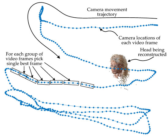
Figure 1.
The need for finding the least motion-blurred (highest quality) image from several images during 3D head reconstruction using a photogrammetry approach. Such a selection process reduces data redundancy and removes distorted images; therefore, the reconstruction process becomes faster and the resulting model is more accurate. In self-recorded videos using smartphones, motion blur is the most affecting image quality factor that can be managed after a video is recorded. So the problem of choosing the highest quality image becomes a motion blur evaluation problem.
The outline of the paper is as follows. In Materials and Methods (Section 2), the proposed method for motion blur evaluation is described; a short description of other image quality evaluation methods that are used as standard is provided; data collection and software tools used is reported. Results (Section 3) gives experimental comparison results of the image quality evaluation methods, and Discussion (Section 4) provides an interpretation of the findings and practical implications. Finally, Section 5 gives the conclusions of this work.
2. Materials and Methods
In this section, we describe a problem of why it is helpful to evaluate motion blur in images that are being used in the photogrammetric reconstruction of the 3D head model. We propose a method that exploits early features of the convolutional neural network (CNN), which performs head localization in images. Additionally, we describe the experimental data collection and preparation process, the creation of training and testing datasets, and outline the evaluation process of image quality evaluation methods.
2.1. Motivation and Method for Finding the Least Motion-Blurred Image
Photogrammetric object reconstruction workflow starts with selecting an appropriate set of images. Images must uniformly cover the space around the object and be of the highest quality. Image sharpness is the most influential factor in image quality. It is very convenient to collect image samples using a smartphone by filming the object. However, taking a video of the object produces oversampling if the camera is moved slowly, or more frames may be distorted by motion blur if the camera is moved faster in a low-lit environment. Some frames may be more affected by motion blur due to an accident shake of a hand or a sudden move. Such frames must be found and removed. Consecutive frames from the video contain nearly duplicate information, but the motion blur distortions may differ. So it would be useful to pick the single highest quality frame from the set of consecutive frames (see Figure 1).
Various factors/settings such as resolution, bitrate, compression, codec, sensor and optics quality, camera ISO, shutter speed, and shooting style determines the quality of the images taken with the camera. Most of them are fixed during a single video, except for shooting style, which can introduce motion blur distortions. So the motion blur can be singled out as the distortion that affects image quality. In order to pick the image that is of maximum quality, as an alternative objective, we can aim to find an image that is corrupted the least by motion blur.
The solution to the problem of finding the highest quality image in the set of images is a method that ranks images according to motion blur distortion level and takes the least distorted image.
2.1.1. Proposed Method
A suitable method would be capable of finding the least motion-blurred image by evaluating the relevant image region. If the background of the image is not static, the object (human head, in our case) should be reconstructed using only the part of the image without the background. Having non-static background is the typical situation when the head is imaged by a handheld device and the head is not immobilized. So the background can be eliminated by detecting the region of the head. A head detector is necessary for such a situation. If the head detector is a convolutional neural network (CNN), it is possible to reuse activations of the convolutional layers as features for other tasks other than head detection (Figure 2). Having information about the head’s location in the image, we can gather only relevant parts of feature maps, i.e., parts that are spatially corresponding to the area in the input image where the head is located (Figure 3).
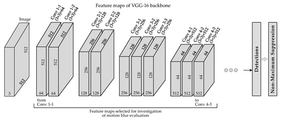
Figure 2.
Partial structure of the convolutional neural network (CNN) model used for human head detection. Features from the first 10 feature maps (outputs of convolutional layers) of the VGG-16 backbone were investigated for suitability to predict motion blur level in the presented image. Names and filter shapes of the convolutional layers are given above the boxes that denote feature maps. The numbers in the boxes specify the shape of the feature maps.
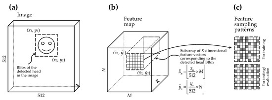
Figure 3.
A diagram explaining the sampling process of features for image quality (motion blur level) evaluation that is based on the LightGBM ranker model. At first, a subarray of K-dimensional feature vectors (part of the feature map) (b) corresponding to the detected head BBox in the input image (a) is determined. The said region of the feature map describes the image patch containing the face. The spatial position of the region in the feature map (b) is relatively the same (proportional) as the position of the head’s bounding box (BBox) in the image (a). Later, only part of the feature vectors from the region are selected (c): feature vectors randomly sampled for the training dataset and uniformly sampled for testing/evaluation.
Image features that define sharpness or motion blur should be found in lower-level image details. These image details should be encoded by the early features of the CNN. Later layers of the CNN encode progressively higher-level structural information about the object it learned to detect. So we will test the first ten feature maps of the CNN for their suitability to provide useful features for the motion blur evaluation of the input image. The CNN head detector [81] used in the experiment is a single-shot detector (SSD) [82] with the VGG-16 [83] backbone. The model adopted in this research was developed by the authors of LAEO-Net [84]. Shapes of the feature maps and names of the convolutional layers that generated these maps are provided in Figure 2 and Table 1.

Table 1.
Summary of the CNN’s first 10 feature maps that were investigated for suitability to provide useful information for prediction of image quality. The number of channels of the feature map determines the dimensionality of the sampled feature vector.
After the head is detected in the image, the corresponding spatial region can be located in the feature map. Features from this region can be used to score an image for motion blur level in the head’s region of an image. All features from the region or just a subset of features could be used. As the spatial size of feature maps reduces twice after each max-pooling, the region that corresponds to the head region also gets smaller. In order to equalize the number of features from different feature maps and to decrease the amount of training data, we chose to sample 50 features from the region for the train set and 100 features for the test set. The sampling pattern was different as well. For the training, features were sampled from the region randomly (see Figure 3c). This strategy additionally should work as overfitting prevention by impeding the model from catching some patterns in the data related to facial features. Feature sampling for testing is performed using a uniform pattern (see Figure 3c). Differences in feature vectors from the same or near similar face locations will ultimately describe mostly quality-related image patterns because quality-unrelated image patterns are near constant.
The method will be picking the least motion-blurred image from the set of images; therefore, rank-1 performance (right image is returned as top-1 prediction) is important, but not the absolute predicted score of image quality. A ranking algorithm in this situation solves the problem. We chose the LightGBM ranker model for learning to score images according to their motion blur distortions. Traditional gradient boosting decision tree was used, which is implemented in Python’s lightgbm package as LGBMRanker class. LambdaRank was used as an objective function. During the construction of the gradient boosting model, the maximum tree leaves for the base learners parameter (num_leaves) was set to 41, boosting learning rate (learning_rate) was set to 0.02, and the number of boosted trees to fit (n_estimators) was set to 10,000. The collection and construction of the training set are described in Section 2.3.
After the ranker model is trained, the key steps of the image quality evaluation using the proposed method are the following:
- Detection of the head region (BBox) (the BBox found in the head’s background removal step is reused).
- Limiting the feature map of the L-th convolutional layer to the region corresponding to the detected head BBox, we get a subarray of K-dimensional feature vectors.
- A subset of 100 feature vectors is uniformly sampled from the subarray of K-dimensional feature vectors for testing/evaluation. For comparison, a subset of 50 feature vectors is randomly sampled for training data.
- Sampled features are provided as inputs for the LightGBM ranker model during the inference (image quality assessment). For comparison, sampled features together with the outputs (ranking information) are given to the LightGBM ranker model during training.
- Making a decision: a higher score indicates less motion blur (better quality).
2.1.2. Standard Methods
Performance of the proposed image quality evaluation method’s variants was compared to the standard methods—fast image quality evaluation using image sharpness as a proxy [85], a method used in the previous study [86], and no-reference image quality metrics (BRISQUE [78], NIQE [79], PIQE [80]). All these methods compute some quality value without a comparison of the image of interest to some reference image. In a situation when we want to find the least motion-blurred (highest quality) image in a group of images that are slightly different (consecutive frames), we do not possess an image that could serve as a reference.
Image Sharpness as Image Quality Proxy
This method was used for the measurement of image sharpness, which was used as an estimate of image quality. The image quality evaluation was required in order to perform the selection of a suitable subset of frames to be passed to the 3D head reconstruction algorithm [86].
The key steps of the image sharpness evaluation method were:
- Detection of the head region (BBox);
- Determination of region of interest (RoI) parameters: RoI is a square and its size is the smaller edge of the head’s BBox;
- Cropping the RoI from the image and resizing it to px image patch;
- Filtering the cropped and resized patch using a Laplacian of Gaussian (LoG) filter ( filter size, );
- Calculating the variance of the filtered patch;
- Making a decision: a larger variance represents a higher image sharpness, hence less motion blur.
No Reference Image Quality Metrics
This group of image quality evaluation methods does not require a reference image to analyze the target image and is also called blind methods. Blind methods use statistical features of the image to assess the image quality. Three methods were included in the pool of image quality evaluators: BRISQUE [78], NIQE [79], and PIQE [80]. Matlab Image Processing Toolbox implementation of these methods was used in experiments [87].
Each metric has its own strengths when analyzing different types of images. Comparing the performance of these different metrics on the validation image set could be the way of choosing the best metric for a particular dataset.
A short description of the used blind image quality evaluation methods:
- BRISQUE—Blind/Referenceless Image Spatial Quality Evaluator [78]. BRISQUE is a model that is trained on databases of distorted images, and it employs an "opinion-aware" approach that assigns subjective quality scores to the training sets.
- NIQE—Natural Image Quality Evaluator [79]. The NIQE model is trained on undistorted images, therefore it can assess the quality of images with arbitrary distortions and does not rely on human opinions when measuring image quality. However, this system does not score images based on the subjective quality scores of viewers; hence, the NIQE score might not be as accurate in predicting human perception of quality.
- PIQE—Perception-based Image Quality Evaluator [80]. The PIQE algorithm is unsupervised, meaning it does not require a trained model. It is also opinion unaware. PIQE is suitable for measuring the quality of images with arbitrary distortion. Mostly it performs similarly to NIQE.
The key steps of the image quality evaluation using blind methods:
- Detection of the head region (BBox);
- Determination of region of interest (RoI) parameters: RoI is a square and its size is the shorter edge of the head’s BBox;
- Cropping the RoI from the image and resizing it to px image patch;
- Providing the patch as input for the BRISQUE, NIQE, or PIQE method;
- Making a decision: a smaller score indicates better perceptual quality.
2.2. Evaluation of the Methods Used for Determination of the Less Motion-Blurred Image
Evaluation of the proposed and standard methods for finding less motion-blurred (better quality) images was performed using testing data. A description of testing dataset preparation is presented in Section 2.3.
At the beginning of the photogrammetry pipeline, we want to select only necessary and of the highest quality images for the object reconstruction (see Figure 1). Picking the highest quality image (which, in our case, we defined as having the least motion blur distortions) from a set of images means sorting these images according to their quality and choosing the best one. The test set is constructed so that the method should pick an image from a pair of images. The method assigns some ranking scores to the images, and the appropriate image is chosen. Our current method gives a higher score for less motion-blurred images; the sharpness-based method also gives a higher score for less motion-blurred images. Blind image quality evaluation methods BRISQUE, NIQE, and PIQE provide a smaller score as indicators of better perceptual quality (less motion blur).
The test set is constructed from original images I1 and their augmented versions I2, I3, I4, and I5. All augmented versions are gradually increasingly affected by motion blur. For the evaluation of the methods, all possible combinations of I1–I5 images were generated. Images that are closer by distortion parameters are harder to differentiate into better and worse according to image quality. The harder pairs are I1–I2, I2–I3, I3–I4, and I4–I5. The easier pairs are I1–I3, I1–I4, I1–I5, I2–I4, I2–I5, and I3–I5.
2.3. Data Preparation
The proposed method is based on the machine learning algorithm LightGBM ranker (gradient boosting decision tree), so the development of the method requires training and testing data. Both training and testing datasets contain real and augmented data (real data after augmentation). For both sets, augmentation allows for the simulation of gradually increasing motion blur. Controlled augmentation of the training data helps to increase the robustness of the developed quality evaluation method. Test data augmentation is used to simulate real situations where the method will be used to find the highest quality or least motion-blurred image from the selected set of images.
Real images were extracted from videos that were collected and used in the previous experiment [86], where the methodology for the improvement of 3D head reconstruction was developed, and it was used to propose changes for the general-purpose 3D reconstruction algorithm. Details regarding video collection are presented in the mentioned work, and here we give a short summary.
Smartphone Samsung Galaxy S10+ standard Camera App was used to take videos. In total, 19 videos were captured, varying in acquisition conditions, such as changing the orientation of the smartphone, changing lighting conditions, and stationary or varied backgrounds. The average length of videos was s. The movement pattern of the camera was simulating an effort to make a selfie—zigzagging sideways and moving slowly from top to bottom, making sure all sides of one’s head are captured.
From the set of 19 videos, 15 videos were used for training and four videos for testing. After frame extraction, the training set contained 10,100 initial/original images, and 50,500 images after augmentations. The test set contained 3253 initial images and 16,265 images after augmentations.
The construction of training and test datasets by augmenting the original image is explained in Figure 4. As mentioned before, augmentation of datasets is needed to simulate gradually increasing motion blur distortions. Randomness in the simulation of motion blur effects provides better generalization properties of the LightGBM ranker. Augmentation of test data is needed to simulate real situations where the single best frame should be selected from the consecutive frames.
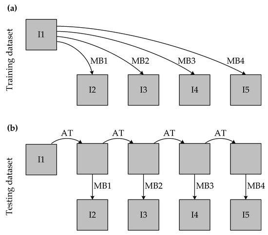
Figure 4.
Construction of the training (a) and test (b) datasets by augmenting original image. Here I1—original image; I2, I3, I4, I5—augmented images; AT—affine transformation of the image; MB1–MB4—motion blurring from the lowest (#1) to the highest (#4) level.
Training data augmentations included only simulations of the linear motion of a camera. The angle of motion was selected randomly, allowing any possible movement direction. The length of the camera motion was 5, 10, 15, and 20 pixels. It is 0.13%, 0.26%, 0.39%, and 0.52% from the largest image dimension. The mentioned motion lengths in Figure 4 are marked as MB1 (motion blur 1), MB2, MB3, and MB4.
Augmentation of test data included the same motion blur distortions but additionally were altered by affine transformation (“AT” in the Figure 4). The parameters of the affine transformation were constant for all transformations of the same initial image but were generated randomly for different initial/original images. The affine transformation was applied cumulatively to the initial image generating four new spatially altered images. This imitates consecutive frames in the video when the camera is moving while taking video. The affine transformation was composed of rotation and X- and Y-translations. Rotation was uniformly sampled from the interval [−0.55, 0.55] degrees. Translations were uniformly sampled from the [−15, 15] pixels range.
Datasets contained all I1–I5 images. However, training and test set exploited images differently. Training of the LightGBM ranker model needs the ranked list of images. The training algorithm received features that were extracted from a list of images ordered in increasing motion blur distortions and grouped by image ID (initial image name). Ranks were provided as targets, with the highest rank assigned to I1 and the lowest to I5. The test set is composed in a way that the developed method should make pairwise comparisons, i.e., select the less motion-blurred (higher quality) image from an image pair. All possible combinations of I1–I5 images were generated for the test set. Images that are closer by distortion parameters are harder to differentiate into better and worse according to image quality. The harder pairs are I1–I2, I2–I3, I3–I4, and I4–I5.
In the exact same way, the test set of real face images was prepared. The test set contained 2976 initial images and 14,880 images after augmentations. The source of real face images was a subset of IMDB-WIKI dataset [88,89]—IMDB cropped images from the first three subfolders, and whose shorter side was longer than 500 pixels.
2.4. Software Used
The software tools and programming languages used in this research are as follows:
- MATLAB programming and numeric computing platform (version R2022a, The Mathworks Inc., Natick, MA, USA) for the implementation of the proposed algorithm (except for training LGBMRanker model), and for data analysis and visualization;
- SSD-based upper-body and head detector (https://github.com/AVAuco/ssd_people accessed on 15 September 2022) [84], for the detection of heads and as a source of features for the image similarity sorting;
- Python (version 3.9.10) (https://www.python.org), (accessed on 15 September 2022) [90], an interpreted, high-level, general-purpose programming language. NumPy, SciPy, and LightGBM packages were used for the machine learning applications (LGBMRanker tool).
3. Results
The results of the experimental comparison of the image quality evaluation methods are summarized in Table 2. Images are of the mannequin head. Results are listed for separate image pair types, for harder image pairs combined (image pairs that are the most similar according to the motion blur level), and for overall results. Harder image pairs are highlighted with a dark background.
Table 2.
Method comparison results of selecting a less motion-blurred image from a pair of images. Images are of the mannequin head. Values in the table are the percentages of selections that were correct. Images in the pairs are the following: I1—original image; I2—AT+MB1 (original image altered by affine transformation + motion blur #1); I3—AT×2+MB2 (original image altered by the previous affine transformation twice + motion blur #2); I4—AT×3+MB3; I5—AT×4+MB4. The best performance in each comparison group (column) is highlighted in red. The dark background of the cells highlights comparison results of harder image pairs, i.e., image pairs that are the most similar according to the motion blur level.
Our proposed method has ten variants (#1–#10)—they differ by the feature map sequence number from which the features were sampled for motion blur evaluation. The “FMx” part in the title of the method designates the source map of the features (see Table 1). Other methods were sharpness (#11), which was used in the previous research [86] to pick the sharpest image from the set. The three remaining methods (#12–#14) are well-known in reference-free (blind) image quality evaluation tasks. The top performing method quite consistently was our proposed LightGBMRanker-based using features from the sixth convolutional layer (Conv 3-2). Actually, a very similar performance was found for LightGBMRanker-based methods that use features from the fifth (Conv 3-1) to ninth (Conv 4-2) convolutional layers. All these methods outperformed all methods used for comparison as standard methods.
An additional experiment was performed to test the potentiality of feature pooling from different feature maps. The results of the experimental comparison of the image quality evaluation methods using combined features from two feature maps are summarized in Table 3. The table presents the average results of harder image pairs and all image pairs. The experimental setup was analogous to the previous experiment. The top-performing method is the one that uses features from the sixth and ninth feature maps. In general, bigger improvements can be observed when features from Conv 3 and Conv 4 convolutional blocks are combined, i.e., one from Conv 3 (Conv 3-1, Conv 3-2, or Conv 3-3) and one from Conv 4 (Conv 4-1, Conv 4-2, or Conv 4-3).
Table 3.
Comparison results of proposed method variants for selecting a less motion-blurred image from a pair of images using pooled features from two different feature maps. Images are of the mannequin head. Values in the table are the percentages of selections that were correct. The table presents the average results of harder image pairs and all image pairs. The best performance is highlighted in red. The dark background of the rows highlights the comparison average results of harder image pairs, i.e., image pairs that are the most similar according to the motion blur level.
Another experiment was conducted using images of real faces. This experiment was identical to the first one. Results are presented in Table 4. In this case, our proposed method remained the top performing, with slight changes to the top positions of the variants of the proposed method. In this situation, the #8 variant is leading instead of the #6, which was at the top when images of a mannequin head were used.
Table 4.
Method comparison results of selecting a less motion-blurred image from a pair of images. Images are of real faces. Values in the table are the percentages of selections that were correct. Images in the pairs are the following: I1—original image; I2—AT+MB1 (original image altered by affine transformation + motion blur #1); I3—AT×2+MB2 (original image altered by the previous affine transformation twice + motion blur #2); I4—AT×3+MB3; I5—AT×4+MB4. The best performance in each comparison group (column) is highlighted in red. The dark background of the cells highlights comparison results of harder image pairs, i.e., image pairs that are the most similar according to the motion blur level.
A graphical summary of the methods’ experimental comparison results presented in Table 2, Table 3 and Table 4 is shown in Figure 5.
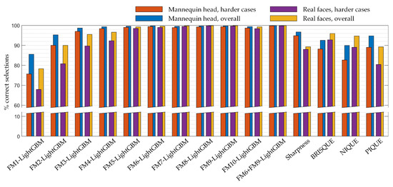
Figure 5.
Graphical summary of all the experimental results of methods comparison. The results are the percentage of correct selections of a less motion-blurred image from a pair of images. Images of a mannequin head and of real faces were used. The chart gives the average performance of the methods tested using all image pairs (overall) and harder image pairs. Harder image pairs are image pairs that are the most similar according to the motion blur level.
4. Discussion
We proposed a method for image quality evaluation of specialized content images. This quality score is required to be able to point to the best-quality image from the set of images. The problem of choosing the best quality images appears during the photogrammetric reconstruction of the human 3D head model when images are collected by making a video of your own or someone else’s head. In this case, some frames are redundant and can be dropped to speed-up reconstruction. Some frames can be motion blurred when the lighting is dimmer and the camera moves faster. Therefore, we would like to pick frames that are the least motion-blurred. A simple solution would be to split the frame sequence into chunks and take a single best-quality frame from each chunk. This procedure would reduce data redundancy as they were covering a small region in space and improve data quality as better quality images were left. The described reduction of frame count will lead to faster and more accurate reconstruction of the head 3D model.
The proposed method reuses features from one of the early convolutional neural network (CNN) layers. This CNN already has its purpose in 3D head reconstruction—it detects the human head. Head detection (in general—object detection) allows for the head’s background to be masked. Background masking is required when it is not static and consequently deteriorates and slows down the photogrammetric reconstruction workflow. So there is no overhead in extracting required features. Experiments showed that early features of CNN are useful in scoring images according to their quality.
We chose to infer some image quality scores as the inverse of motion blur level. Because images were collected via single-take video, many of the image quality-defining factors are fixed: same camera optics, camera sensor, environmental video-taking conditions, and camera settings (ISO, shutter speed). The one factor that strongly influences image quality and in most cases changes is motion blur. It depends on the speed of camera movement, and it is not simple to guarantee the camera’s stable and adequately slow movement while making a video with a smartphone by hand. So the best quality image in the image set is the image with the least motion blur.
The proposed method for image quality evaluation is based on inferring motion blur level from the early features of a CNN-based head detector, using a LightGBM ranker model. The model was trained on synthetically expanded (augmented) real images of a mannequin’s head—augmentation simulated motion blur of various levels and directions. From the one original image via augmentation, four additional images of increasing motion blur lengths were generated. These images were passed to CNN for head detection, and features (activations) from the first ten convolutional layers were collected for the training of the LightGBM ranker model. Features from separate feature maps were used with separate models, so we compared the usefulness of features from different feature maps.
Absolute values of image blurriness are unknown as the ground truth blurriness of the initial image is unknown. The following images, which were generated from the original by simulating motion blur of random direction but fixed length, can be ordered in increasing order of blurriness. So the solution to train the machine learning model was to train the LightGBM ranker model. It does not require an absolute ground truth value of the image property that should be predicted, but only a ranking order. Using this model in inference mode provides a possibility to rank a group of new images according to motion blur distortions in the images and a way to find an image with the lowest motion blur.
Features from the feature maps were sampled from the region that corresponds to the detected region of the head. The bounding box (BBox) of the head in the input image is scaled down the spatial position in the feature proportionally according to the size ratios of the feature map and input image. After finding a region in the feature map that corresponds to the head position, we randomly sample features from that region. Sampling randomly allows for reducing the possibility of overfitting the model to features specific to some facial regions. So it works as a regularization strategy. During inference, features are sampled uniformly in the corresponding head region. Each feature vector is passed to the LightGBM ranker model, and the outputs from the same image are averaged to get a final score that is used to select an image with the largest one.
The results of the first experimental comparison (images of the mannequin head) of image quality evaluation methods show that our proposed method outperformed standard methods: sharpness-based, BRISQUE, NIQUE, and PIQUE. The best-performing variant, FM6-LightGBM of the proposed method, achieved 99.8% rank-1 accuracy, so it reliably finds a less motion-blurred (higher quality) image from the two images in the test set. This method variant was consistently the best performing in almost all pairwise image comparison tests. The variant is based on features from the 6th convolutional layer (Conv 3-2). The only place where it was a runner-up was the first category, where the method must differentiate between I1–I2 images. These images are from a harder comparison set because their quality differs the least. The I1 image is the original image, and the I2 image is the original image affected by the smallest motion blur compared to all images in this experiment. It may be that minor motion blur distortions do not significantly affect image quality. Additionally, the original images were not reviewed to remove lower quality frames, so the minor additional distortions could be that are not imposing quality degradation of the original image. The I1–I2 comparison category was the hardest for all methods, so the lower initial quality of the frames could be the reason.
Additional experiments were performed to compare the methods using images of real faces and to test the potentiality of fusing features from different feature maps. The experiment using images of real faces shows that our proposed method remained the top-performing. There were slight changes in the top positions for the variants of the proposed method—in the situation of real faces, the #8 variant (features from Conv 4-1 convolutional layer) is leading instead of the #6 (features from Conv 3-2 convolutional layer), which was in the top when images of mannequin head were used. This shift is probably due to the change in the overall quality of images but not due to the change from mannequin face to real faces. Images of the mannequin were collected by us at 2–3 times higher resolution than images of real faces from the IMDB-WIKI dataset. To perform similar experiments, images of real faces were upsampled to be of similar resolution to the images of the mannequin head. Consequently, images of real faces contain less higher-frequency components, which are detected in earlier feature maps. The case of lower levels of higher-frequency components additionally explains why the performance of the sharpness-based method dropped in this case.
Experiments on feature pooling from different feature maps show that feature combination is beneficial and increases the performance of our proposed method. In general, greater improvements can be observed when features from Conv 3 and Conv 4 convolutional blocks are combined, i.e., one from Conv 3 block (from Conv 3-1, Conv 3-2, or Conv 3-3 convolutional layers) and one from Conv 4 (from Conv 4-1, Conv 4-2, or Conv 4-3 convolutional layers). Selecting features from the same convolutional block typically does not provide any improvement. It makes sense because features from different scales bring more different information.
Each method that was used as a standard may have its own strengths when analyzing different types of images. Comparing the performance of these different metrics on the validation image set could be the way of choosing the best metric for a particular task or dataset.
The performance of the proposed method could potentially be improved by combining features from more than two feature maps. However, such a design will lead to the increased complexity of the ranker model due to the increased number of input features. It is likely that the dimensionality of the feature vector could be reduced without loss of accuracy.
Further experiments could be done to test the proposed method on natural images. The same method should be able to pick the least motion-blurred image from the group of images. Even the same CNN model could be used as a feature extractor, but features should be sampled from the full area of the feature maps. CNNs trained on natural images (e.g., ImageNet data) could serve as universal feature extractors.
5. Conclusions
Photogrammetric reconstruction of 3D objects requires images of high quality. If we have a large collection of images, it would be useful to drop some frames to reduce data redundancy and eliminate lower-quality images. It would increase reconstruction speed and reconstruction accuracy. A tool for finding better quality images in a group of images would help to reduce said image collection. The most quality-affecting factor in the group of images (frames) that were taken via a single video shot is motion blur. We proposed and experimentally compared the developed method to the other image quality evaluation methods: sharpness-based, BRISQUE, NIQUE, and PIQUE. The proposed method uses activations of one of the early layers of the human head detection CNN model as input features. The model is already doing its job in the 3D head reconstruction workflow for background removal, so the extraction of features has no overhead (features are being reused). The proposed method is based on the LightGBM ranker model. The experimental comparison showed that the developed method outperformed other well-known image quality evaluation methods used in the comparison. Additionally, an experimental comparison shows that features from the fifth to ninth feature maps provided the top results for motion blur evaluation.
Author Contributions
Conceptualization, D.M. and A.S.; methodology, M.T. and D.M.; software, M.T. and D.M.; validation, V.A. and T.S.; formal analysis, M.T., and A.S.; investigation, M.T., D.K.-L. and V.A.; resources, A.S. and D.N.; data curation, M.T. and D.M.; writing—original draft preparation, M.T.; writing—review, editing, M.T., D.K.-L., T.S. and A.S.; visualization, M.T., T.S. and D.M.; supervision, D.M., A.S. and D.N.; project administration, A.S. and D.N. All authors have read and agreed to the published version of the manuscript.
Funding
This research received no external funding.
Institutional Review Board Statement
Not applicable.
Informed Consent Statement
Not applicable.
Data Availability Statement
The data presented in this study are available upon reasonable request from the corresponding author. The data are not publicly available due to privacy issues.
Conflicts of Interest
The author declares no conflict of interest.
Abbreviations
The following abbreviations are used in this manuscript:
| CNN | Convolutional Neural Network |
| SSD | Single Shot Detector |
| FM | Feature Map |
| BBox | Bounding Box |
| RoI | Region of Interest |
| LoG | Laplacian of Gaussian |
| AT | Affine Transformation |
| MB | Motion Blur |
| SfM | Structure from Motion |
References
- Xu, Z.; Wu, T.; Shen, Y.; Wu, L. Three dimentional reconstruction of large cultural heritage objects based on uav video and tls data. Int. Arch. Photogramm. Remote Sens. Spat. Inf. Sci. 2016, 41, 985. [Google Scholar] [CrossRef]
- Matuzevičius, D.; Serackis, A.; Navakauskas, D. Mathematical models of oversaturated protein spots. Elektron. ir elektrotechnika 2007, 73, 63–68. [Google Scholar]
- Matuzevičius, D. Synthetic Data Generation for the Development of 2D Gel Electrophoresis Protein Spot Models. Appl. Sci. 2022, 12, 4393. [Google Scholar] [CrossRef]
- Hamzah, N.B.; Setan, H.; Majid, Z. Reconstruction of traffic accident scene using close-range photogrammetry technique. Geoinf. Sci. J. 2010, 10, 17–37. [Google Scholar]
- Caradonna, G.; Tarantino, E.; Scaioni, M.; Figorito, B. Multi-image 3D reconstruction: A photogrammetric and structure from motion comparative analysis. In Proceedings of the International Conference on Computational Science and Its Applications, Melbourne, Australia, 2–5 July 2018; pp. 305–316. [Google Scholar]
- Žuraulis, V.; Matuzevičius, D.; Serackis, A. A method for automatic image rectification and stitching for vehicle yaw marks trajectory estimation. Promet-Traffic Transp. 2016, 28, 23–30. [Google Scholar] [CrossRef]
- Sledevič, T.; Serackis, A.; Plonis, D. FPGA Implementation of a Convolutional Neural Network and Its Application for Pollen Detection upon Entrance to the Beehive. Agriculture 2022, 12, 1849. [Google Scholar] [CrossRef]
- Genchi, S.A.; Vitale, A.J.; Perillo, G.M.; Delrieux, C.A. Structure-from-motion approach for characterization of bioerosion patterns using UAV imagery. Sensors 2015, 15, 3593–3609. [Google Scholar] [CrossRef]
- Mistretta, F.; Sanna, G.; Stochino, F.; Vacca, G. Structure from motion point clouds for structural monitoring. Remote Sens. 2019, 11, 1940. [Google Scholar] [CrossRef]
- Varna, D.; Abromavičius, V. A System for a Real-Time Electronic Component Detection and Classification on a Conveyor Belt. Appl. Sci. 2022, 12, 5608. [Google Scholar] [CrossRef]
- Matuzevicius, D.; Navakauskas, D. Feature selection for segmentation of 2-D electrophoresis gel images. In Proceedings of the IEEE 2008 11th International Biennial Baltic Electronics Conference, Tallinn, Estonia, 6–8 October 2008; pp. 341–344. [Google Scholar]
- Zeraatkar, M.; Khalili, K. A Fast and Low-Cost Human Body 3D Scanner Using 100 Cameras. J. Imaging 2020, 6, 21. [Google Scholar] [CrossRef] [PubMed]
- Straub, J.; Kading, B.; Mohammad, A.; Kerlin, S. Characterization of a large, low-cost 3D scanner. Technologies 2015, 3, 19–36. [Google Scholar] [CrossRef]
- Straub, J.; Kerlin, S. Development of a large, low-cost, instant 3D scanner. Technologies 2014, 2, 76–95. [Google Scholar] [CrossRef]
- Özyeşil, O.; Voroninski, V.; Basri, R.; Singer, A. A survey of structure from motion*. Acta Numer. 2017, 26, 305–364. [Google Scholar] [CrossRef]
- Iglhaut, J.; Cabo, C.; Puliti, S.; Piermattei, L.; O’Connor, J.; Rosette, J. Structure from motion photogrammetry in forestry: A review. Curr. For. Rep. 2019, 5, 155–168. [Google Scholar] [CrossRef]
- Wei, Y.M.; Kang, L.; Yang, B.; Wu, L.D. Applications of structure from motion: A survey. J. Zhejiang Univ. Sci. C 2013, 14, 486–494. [Google Scholar] [CrossRef]
- Westoby, M.J.; Brasington, J.; Glasser, N.F.; Hambrey, M.J.; Reynolds, J.M. ‘Structure-from-Motion’photogrammetry: A low-cost, effective tool for geoscience applications. Geomorphology 2012, 179, 300–314. [Google Scholar] [CrossRef]
- Jiang, R.; Jáuregui, D.V.; White, K.R. Close-range photogrammetry applications in bridge measurement: Literature review. Measurement 2008, 41, 823–834. [Google Scholar] [CrossRef]
- Barbero-García, I.; Cabrelles, M.; Lerma, J.L.; Marqués-Mateu, Á. Smartphone-based close-range photogrammetric assessment of spherical objects. Photogramm. Rec. 2018, 33, 283–299. [Google Scholar] [CrossRef]
- Fawzy, H.E.D. The accuracy of mobile phone camera instead of high resolution camera in digital close range photogrammetry. Int. J. Civ. Eng. Technol. (IJCIET) 2015, 6, 76–85. [Google Scholar]
- Vacca, G. Overview of open source software for close range photogrammetry. In Proceedings of the 2019 Free and Open Source Software for Geospatial, FOSS4G 2019, International Society for Photogrammetry and Remote Sensing, Bucharest, Romania, 26–30 August 2019; Volume 42, pp. 239–245. [Google Scholar]
- Griwodz, C.; Gasparini, S.; Calvet, L.; Gurdjos, P.; Castan, F.; Maujean, B.; Lillo, G.D.; Lanthony, Y. AliceVision Meshroom: An open-source 3D reconstruction pipeline. In Proceedings of the 12th ACM Multimedia Systems Conference-MMSys ’21, Istanbul, Turkey, 28 September–1 October 2021; ACM Press: New York, NY, USA, 2021. [Google Scholar] [CrossRef]
- Schönberger, J.L.; Frahm, J.M. Structure-from-Motion Revisited. In Proceedings of the Conference on Computer Vision and Pattern Recognition (CVPR), Las Vegas, NV, USA, 27–30 June 2016. [Google Scholar]
- Schönberger, J.L.; Zheng, E.; Pollefeys, M.; Frahm, J.M. Pixelwise View Selection for Unstructured Multi-View Stereo. In Proceedings of the European Conference on Computer Vision (ECCV), Amsterdam, The Netherlands, 11–14 October 2016. [Google Scholar]
- Wu, C. VisualSFM: A Visual Structure from Motion System. Available online: http://ccwu.me/vsfm/ (accessed on 5 December 2022).
- Moulon, P.; Monasse, P.; Perrot, R.; Marlet, R. OpenMVG: Open multiple view geometry. In Proceedings of the International Workshop on Reproducible Research in Pattern Recognition, Cancún, Mexico, 4 December 2016; Springer: Berlin/Heidelberg, Germany, 2016; pp. 60–74. [Google Scholar]
- Regard3D. Available online: www.regard3d.org/ (accessed on 5 December 2022).
- OpenDroneMap—A Command Line Toolkit to Generate Maps, Point Clouds, 3D Models and DEMs from Drone, Balloon or Kite Images. Available online: https://github.com/OpenDroneMap/ODM/ (accessed on 5 December 2022).
- Fuhrmann, S.; Langguth, F.; Goesele, M. MVE-A Multi-View Reconstruction Environment. In Proceedings of the Eurographics Workshop on Graphics and Cultural Heritage, Darmstadt, Germany, 6–8 October 2014; pp. 11–18. [Google Scholar]
- Rupnik, E.; Daakir, M.; Deseilligny, M.P. MicMac–a free, open-source solution for photogrammetry. Open Geospat. Data Softw. Stand. 2017, 2, 1–9. [Google Scholar] [CrossRef]
- Nikolov, I.; Madsen, C. Benchmarking close-range structure from motion 3D reconstruction software under varying capturing conditions. In Proceedings of the Euro-Mediterranean Conference; Springer: Berlin/Heidelberg, Germany, 2016; pp. 15–26. [Google Scholar]
- Pixpro. Available online: https://www.pix-pro.com/ (accessed on 5 December 2022).
- Agisoft. Metashape. Available online: https://www.agisoft.com/ (accessed on 5 December 2022).
- 3Dflow. 3DF Zephyr. Available online: https://www.3dflow.net/ (accessed on 5 December 2022).
- Bentley. ContextCapture. Available online: https://www.bentley.com/software/contextcapture-viewer/ (accessed on 5 December 2022).
- Autodesk. ReCap. Available online: https://www.autodesk.com/products/recap/ (accessed on 5 December 2022).
- CapturingReality. RealityCapture. Available online: https://www.capturingreality.com/ (accessed on 5 December 2022).
- Technologies, P. PhotoModeler. Available online: https://www.photomodeler.com/ (accessed on 5 December 2022).
- Pix4D. PIX4Dmapper. Available online: https://www.pix4d.com/product/pix4dmapper-photogrammetry-software/ (accessed on 5 December 2022).
- DroneDeploy. Available online: https://www.dronedeploy.com/ (accessed on 5 December 2022).
- Trimble. Inpho. Available online: https://geospatial.trimble.com/products-and-solutions/trimble-inpho (accessed on 5 December 2022).
- OpenDroneMap. WebODM. Available online: https://www.opendronemap.org/webodm/ (accessed on 5 December 2022).
- AG, P. Elcovision 10. Available online: https://en.elcovision.com/ (accessed on 5 December 2022).
- Trojnacki, M.; Dąbek, P.; Jaroszek, P. Analysis of the Influence of the Geometrical Parameters of the Body Scanner on the Accuracy of Reconstruction of the Human Figure Using the Photogrammetry Technique. Sensors 2022, 22, 9181. [Google Scholar] [CrossRef] [PubMed]
- Mitchell, H. Applications of digital photogrammetry to medical investigations. ISPRS J. Photogramm. Remote Sens. 1995, 50, 27–36. [Google Scholar] [CrossRef]
- Barbero-García, I.; Pierdicca, R.; Paolanti, M.; Felicetti, A.; Lerma, J.L. Combining machine learning and close-range photogrammetry for infant’s head 3D measurement: A smartphone-based solution. Measurement 2021, 182, 109686. [Google Scholar] [CrossRef]
- Barbero-García, I.; Lerma, J.L.; Mora-Navarro, G. Fully automatic smartphone-based photogrammetric 3D modelling of infant’s heads for cranial deformation analysis. ISPRS J. Photogramm. Remote Sens. 2020, 166, 268–277. [Google Scholar] [CrossRef]
- Lerma, J.L.; Barbero-García, I.; Marqués-Mateu, Á.; Miranda, P. Smartphone-based video for 3D modelling: Application to infant’s cranial deformation analysis. Measurement 2018, 116, 299–306. [Google Scholar] [CrossRef]
- Barbero-García, I.; Lerma, J.L.; Marqués-Mateu, Á.; Miranda, P. Low-cost smartphone-based photogrammetry for the analysis of cranial deformation in infants. World Neurosurg. 2017, 102, 545–554. [Google Scholar] [CrossRef] [PubMed]
- Ariff, M.F.M.; Setan, H.; Ahmad, A.; Majid, Z.; Chong, A. Measurement of the human face using close-range digital photogrammetry technique. In Proceedings of the International Symposium and Exhibition on Geoinformation, GIS Forum, Penang, Malaysia, 27–29 September 2005. [Google Scholar]
- Schaaf, H.; Malik, C.Y.; Streckbein, P.; Pons-Kuehnemann, J.; Howaldt, H.P.; Wilbrand, J.F. Three-dimensional photographic analysis of outcome after helmet treatment of a nonsynostotic cranial deformity. J. Craniofacial Surg. 2010, 21, 1677–1682. [Google Scholar] [CrossRef]
- Utkualp, N.; Ercan, I. Anthropometric measurements usage in medical sciences. BioMed Res. Int. 2015, 2015. [Google Scholar] [CrossRef]
- Galantucci, L.M.; Lavecchia, F.; Percoco, G. 3D Face measurement and scanning using digital close range photogrammetry: Evaluation of different solutions and experimental approaches. In Proceedings of the International Conference on 3D Body Scanning Technologies, Lugano, Switzerland, 9–20 October 2010; p. 52. [Google Scholar]
- Galantucci, L.M.; Percoco, G.; Di Gioia, E. New 3D digitizer for human faces based on digital close range photogrammetry: Application to face symmetry analysis. Int. J. Digit. Content Technol. Its Appl. 2012, 6, 703. [Google Scholar]
- Jones, P.R.; Rioux, M. Three-dimensional surface anthropometry: Applications to the human body. Opt. Lasers Eng. 1997, 28, 89–117. [Google Scholar] [CrossRef]
- Löffler-Wirth, H.; Willscher, E.; Ahnert, P.; Wirkner, K.; Engel, C.; Loeffler, M.; Binder, H. Novel anthropometry based on 3D-bodyscans applied to a large population based cohort. PLoS ONE 2016, 11, e0159887. [Google Scholar] [CrossRef] [PubMed]
- Clausner, T.; Dalal, S.S.; Crespo-García, M. Photogrammetry-based head digitization for rapid and accurate localization of EEG electrodes and MEG fiducial markers using a single digital SLR camera. Front. Neurosci. 2017, 11, 264. [Google Scholar] [CrossRef] [PubMed]
- Abromavičius, V.; Serackis, A. Eye and EEG activity markers for visual comfort level of images. Biocybern. Biomed. Eng. 2018, 38, 810–818. [Google Scholar] [CrossRef]
- Abromavicius, V.; Serackis, A.; Katkevicius, A.; Plonis, D. Evaluation of EEG-based Complementary Features for Assessment of Visual Discomfort based on Stable Depth Perception Time. Radioengineering 2018, 27. [Google Scholar] [CrossRef]
- Leipner, A.; Obertová, Z.; Wermuth, M.; Thali, M.; Ottiker, T.; Sieberth, T. 3D mug shot—3D head models from photogrammetry for forensic identification. Forensic Sci. Int. 2019, 300, 6–12. [Google Scholar] [CrossRef] [PubMed]
- Battistoni, G.; Cassi, D.; Magnifico, M.; Pedrazzi, G.; Di Blasio, M.; Vaienti, B.; Di Blasio, A. Does Head Orientation Influence 3D Facial Imaging? A Study on Accuracy and Precision of Stereophotogrammetric Acquisition. Int. J. Environ. Res. Public Health 2021, 18, 4276. [Google Scholar] [CrossRef]
- Trujillo-Jiménez, M.A.; Navarro, P.; Pazos, B.; Morales, L.; Ramallo, V.; Paschetta, C.; De Azevedo, S.; Ruderman, A.; Pérez, O.; Delrieux, C.; et al. body2vec: 3D Point Cloud Reconstruction for Precise Anthropometry with Handheld Devices. J. Imaging 2020, 6, 94. [Google Scholar] [CrossRef]
- Heymsfield, S.B.; Bourgeois, B.; Ng, B.K.; Sommer, M.J.; Li, X.; Shepherd, J.A. Digital anthropometry: A critical review. Eur. J. Clin. Nutr. 2018, 72, 680–687. [Google Scholar] [CrossRef]
- Perini, T.A.; Oliveira, G.L.D.; Ornellas, J.D.S.; Oliveira, F.P.D. Technical error of measurement in anthropometry. Rev. Bras. De Med. Do Esporte 2005, 11, 81–85. [Google Scholar] [CrossRef]
- Kouchi, M.; Mochimaru, M. Errors in landmarking and the evaluation of the accuracy of traditional and 3D anthropometry. Appl. Ergon. 2011, 42, 518–527. [Google Scholar] [CrossRef]
- Zhuang, Z.; Shu, C.; Xi, P.; Bergman, M.; Joseph, M. Head-and-face shape variations of US civilian workers. Appl. Ergon. 2013, 44, 775–784. [Google Scholar] [CrossRef]
- Kuo, C.C.; Wang, M.J.; Lu, J.M. Developing sizing systems using 3D scanning head anthropometric data. Measurement 2020, 152, 107264. [Google Scholar] [CrossRef]
- Pang, T.Y.; Lo, T.S.T.; Ellena, T.; Mustafa, H.; Babalija, J.; Subic, A. Fit, stability and comfort assessment of custom-fitted bicycle helmet inner liner designs, based on 3D anthropometric data. Appl. Ergon. 2018, 68, 240–248. [Google Scholar] [CrossRef] [PubMed]
- Ban, K.; Jung, E.S. Ear shape categorization for ergonomic product design. Int. J. Ind. Ergon. 2020, 102962. [Google Scholar] [CrossRef]
- Verwulgen, S.; Lacko, D.; Vleugels, J.; Vaes, K.; Danckaers, F.; De Bruyne, G.; Huysmans, T. A new data structure and workflow for using 3D anthropometry in the design of wearable products. Int. J. Ind. Ergon. 2018, 64, 108–117. [Google Scholar] [CrossRef]
- Simmons, K.P.; Istook, C.L. Body measurement techniques: Comparing 3D body-scanning and anthropometric methods for apparel applications. J. Fash. Mark. Manag. 2003, 7, 306–332. [Google Scholar] [CrossRef]
- Zhao, Y.; Mo, Y.; Sun, M.; Zhu, Y.; Yang, C. Comparison of three-dimensional reconstruction approaches for anthropometry in apparel design. J. Text. Inst. 2019. [Google Scholar] [CrossRef]
- Psikuta, A.; Frackiewicz-Kaczmarek, J.; Mert, E.; Bueno, M.A.; Rossi, R.M. Validation of a novel 3D scanning method for determination of the air gap in clothing. Measurement 2015, 67, 61–70. [Google Scholar] [CrossRef]
- Paquette, S. 3D scanning in apparel design and human engineering. IEEE Comput. Graph. Appl. 1996, 16, 11–15. [Google Scholar] [CrossRef]
- Yao, G.; Huang, P.; Ai, H.; Zhang, C.; Zhang, J.; Zhang, C.; Wang, F. Matching wide-baseline stereo images with weak texture using the perspective invariant local feature transformer. J. Appl. Remote Sens. 2022, 16, 036502. [Google Scholar] [CrossRef]
- Wei, L.; Huo, J. A Global fundamental matrix estimation method of planar motion based on inlier updating. Sensors 2022, 22, 4624. [Google Scholar] [CrossRef] [PubMed]
- Mittal, A.; Moorthy, A.K.; Bovik, A.C. No-reference image quality assessment in the spatial domain. IEEE Trans. Image Process. 2012, 21, 4695–4708. [Google Scholar] [CrossRef] [PubMed]
- Mittal, A.; Soundararajan, R.; Bovik, A.C. Making a “completely blind” image quality analyzer. IEEE Signal Process. Lett. 2012, 20, 209–212. [Google Scholar] [CrossRef]
- Venkatanath, N.; Praneeth, D.; Bh, M.C.; Channappayya, S.S.; Medasani, S.S. Blind image quality evaluation using perception based features. In Proceedings of the IEEE 2015 Twenty First National Conference on Communications (NCC), Bombay, India, 27 February–1 March 2015; pp. 1–6. [Google Scholar]
- Kumar, A.; Kaur, A.; Kumar, M. Face detection techniques: A review. Artif. Intell. Rev. 2019, 52, 927–948. [Google Scholar] [CrossRef]
- Liu, W.; Anguelov, D.; Erhan, D.; Szegedy, C.; Reed, S.; Fu, C.Y.; Berg, A.C. SSD: Single Shot MultiBox Detector. In Proceedings of the European Conference on Computer Vision, ECCV’2016, Amsterdam, The Netherlands, 8–16 October 2016; pp. 21–37. [Google Scholar]
- Simonyan, K.; Zisserman, A. Very deep convolutional networks for large-scale image recognition. arXiv 2014, arXiv:1409.1556. [Google Scholar]
- Marin-Jimenez, M.J.; Kalogeiton, V.; Medina-Suarez, P.; Zisserman, A. LAEO-Net: Revisiting people Looking At Each Other in videos. In Proceedings of the IEEE/CVF Conference on Computer Vision and Pattern Recognition (CVPR), Long Beach, CA, USA, 15–20 June 2019; pp. 3477–3485. [Google Scholar]
- Santos, A.; Ortiz de Solórzano, C.; Vaquero, J.J.; Pena, J.M.; Malpica, N.; del Pozo, F. Evaluation of autofocus functions in molecular cytogenetic analysis. J. Microsc. 1997, 188, 264–272. [Google Scholar] [CrossRef] [PubMed]
- Matuzevičius, D.; Serackis, A. Three-Dimensional Human Head Reconstruction Using Smartphone-Based Close-Range Video Photogrammetry. Appl. Sci. 2021, 12, 229. [Google Scholar] [CrossRef]
- The MathWorks® Image Processing Toolbox; MathWorks: Natick, MA, USA, 2022.
- Rothe, R.; Timofte, R.; Gool, L.V. Deep expectation of real and apparent age from a single image without facial landmarks. Int. J. Comput. Vis. 2018, 126, 144–157. [Google Scholar] [CrossRef]
- Rothe, R.; Timofte, R.; Gool, L.V. DEX: Deep EXpectation of apparent age from a single image. In Proceedings of the IEEE International Conference on Computer Vision Workshops (ICCVW), Santiago, Chile, 7–13 December 2015. [Google Scholar]
- Van Rossum, G.; Drake, F.L. Python 3 Reference Manual; CreateSpace: Scotts Valley, CA, USA, 2009. [Google Scholar]


Disclaimer/Publisher’s Note: The statements, opinions and data contained in all publications are solely those of the individual author(s) and contributor(s) and not of MDPI and/or the editor(s). MDPI and/or the editor(s) disclaim responsibility for any injury to people or property resulting from any ideas, methods, instructions or products referred to in the content. |
© 2023 by the authors. Licensee MDPI, Basel, Switzerland. This article is an open access article distributed under the terms and conditions of the Creative Commons Attribution (CC BY) license (https://creativecommons.org/licenses/by/4.0/).