Convolutional Neural Network-Based Classification of Steady-State Visually Evoked Potentials with Limited Training Data

Abstract

One approach employed in brain–computer interfaces (BCIs) involves the use of steady-state visual evoked potentials (SSVEPs). This article examines the capability of artificial intelligence, specifically convolutional neural networks (CNNs), to improve SSVEP detection in BCIs. Implementing CNNs for this task does not require specialized knowledge. The subsequent layers of the CNN extract valuable features and perform classification. Nevertheless, a significant number of training examples are typically required, which can pose challenges in the practical application of BCI. This article examines the possibility of using a CNN in combination with data augmentation to address the issue of a limited training dataset. The data augmentation method that we applied is based on the spectral analysis of the electroencephalographic signals (EEG). Initially, we constructed the spectral representation of the EEG signals. Subsequently, we generated new signals by applying random amplitude and phase variations, along with the addition of noise characterized by specific parameters. The method was tested on a set of real EEG signals containing SSVEPs, which were recorded during stimulation by light-emitting diodes (LEDs) at frequencies of 5, 6, 7, and 8 Hz. We compared the classification accuracy and information transfer rate (ITR) across various machine learning approaches using both real training data and data generated with our augmentation method. Our proposed augmentation method combined with a convolutional neural network achieved a high classification accuracy of 0.72. In contrast, the linear discriminant analysis (LDA) method resulted in an accuracy of 0.59, while the canonical correlation analysis (CCA) method yielded 0.57. Additionally, the proposed approach facilitates the training of CNNs to perform more effectively in the presence of various EEG artifacts.

1. Introduction

Brain–computer interfaces (BCI) have been continuously developing over twelve years. They enable communication for completely paralyzed people, but at the same time they are increasingly being used by healthy individuals, for example in the entertainment industry [1,2,3,4,5]. BCI employs several EEG potentials. The most common are brain potentials associated with movement (ERD/ERS), P300 potentials, and steady-state visually evoked potentials (SSVEP) [6,7]. SSVEP-based BCIs are relatively common because they are easy to use. They require the user to observe flashing lights at a given frequency. The stimulators can be specially constructed panels with LEDs or LCD screens [8,9,10]. SSVEPs appear in the back of the head, where the visual cortex is located [11]. Many SSVEP-based interfaces utilize a limited number of electrodes, typically positioned over the visual cortex at the back of the head, with O₁, O₂, and O_z being the most commonly used [12]. We can observe the dominance of brain waves with the same frequencies as stimuli and their harmonics in the visual cortex. Power spectral density analysis (PSDA) methods [13] are the most widely used for feature extraction to distinguish stimulation frequencies. Dedicated methods have also been developed, such as canonical correlation analysis (CCA) [14] or simplified matching pursuit (sMP) [15].

Typically, a calibration session is performed in BCI systems to train the classifier to detect specific patterns. These patterns may differ for each person and each EEG signal registration. For example, each user may have slightly different SSVEPs (amplitudes). This may be due to anatomical and physiological differences (thickness of the skull, properties of head skin, structure of the cerebral cortex). Differences in the registration of SSVEPs may appear even for the same person (different electrode placements, skin contact surface with the electrode, stimulus power). In a calibration session, a user observes the known stimulation frequencies. The recorded EEG signal for a given stimulation frequency allows for the extraction of features to train the system. BCI can also run without a calibration session. In this case, we analyze the stimulation frequencies and their harmonics in the EEG signal. This simplification, however, results in lower efficiency of the system [16,17].

Features for SSVEP-based BCIs may encompass specific frequencies and their harmonics [18]. These features are utilized to train the classification and decision-making systems. For the SSVEP interface, numerous standard machine learning techniques are employed, including k-nearest neighbors (K-NN), linear discriminant analysis (LDA), quadratic discriminant analysis (QDA), support vector machines (SVM), and multilayer perceptron (MLP), among others [19]. Additionally, deep learning techniques are used for this purpose, with convolutional neural networks (CNN), long short-term memory networks (LSTM), and autoencoders (AE) being the most common structures [20]. Deep learning techniques offer several benefits, such as improved classification results and the capability for automatic feature extraction from signals and images, as seen with CNNs [21]. However, the disadvantages of deep learning are notable, including the necessity for a large dataset for training and the extensive time required for network training [22]. Given that deep learning techniques demand substantial training data, the development of effective methods for augmenting EEG data recorded during calibration sessions presents a significant challenge.

In recent years, numerous solutions employing convolutional neural networks (CNNs) for SSVEP detection have been developed. The study referenced in [23], discusses a machine learning approach for detecting SSVEP using a minimal number of channels. In [24], a proposed CNN model is compared with a standard neural network and other leading methods for SSVEP decoding—such as canonical correlation analysis (CCA), a CCA-based classifier, a multivariate synchronization index, and CCA combined with a k-nearest neighbors (K-NN) classifier—in an offline analysis. The research in [25] introduces a fusion algorithm (CCA-CWT-SVM) that integrates CCA, continuous wavelet transform (CWT), and support vector machine (SVM) to enhance classification accuracy for targetless stimuli when a single feature extraction method is used. In [26], a novel deep neural network (DNN) architecture is presented that processes multi-channel SSVEP signals by convolving across sub-bands of harmonics, channels, time, and classifies the signals at the fully connected layer. In [27], a classification method based on a convolutional neural network (CNN) was presented to enhance the detection accuracy of SSVEP amid competing stimuli. The method was evaluated using a seven-class SSVEP dataset from ten healthy participants. The study in [28] demonstrates the use of a compact convolutional neural network (Compact-CNN), which requires only raw EEG signals for automatic feature extraction, in decoding signals from a 12-class SSVEP dataset without user-specific calibration. In [29], a nonlinear model based on a convolutional neural network, named convolutional correlation analysis (Conv-CA), was introduced. Unlike pure deep learning models, Conv-CA combines a CNN with a unique correlation layer, where the CNN transforms multiple EEG channels into a single signal, and the correlation layer computes the correlation coefficients between this transformed signal and the reference signals. In [30], a complex-valued convolutional neural network (CVCNN) is proposed to overcome the limitation of SSVEP-based BCIs, which is the available stimulation frequency. The presented results demonstrate that the proposed method not only overcomes the limitation of the stimulation frequency but also outperforms conventional SSVEP feature extraction methods. Articles [31,32] introduce a convolutional neural network (CNN) specifically designed to learn the relationship between EEG signals and the templates corresponding to each stimulus frequency of SSVEPs. The effectiveness of the proposed method is validated by comparison with the standard canonical correlation analysis (CCA) and other state-of-the-art methods for decoding SSVEPs (i.e., CNN and task-related component analysis, TRCA, Vaughan, ON, Canada) using actual SSVEP datasets. The study confirmed the efficiency of the proposed CNN-based network in decoding SSVEPs. A comprehensive list of various algorithms used for SSVEP classification, along with signal recording methods, number of channels, number of users, and classification accuracy, is available in the work cited as [23].

The analysis of the literature indicates that the use of convolutional neural networks allows for satisfactory SSVEP recognition accuracy. However, the practical application of CNNs has been investigated only on a limited basis. This limitation pertains to issues such as the small number of electrodes, extended training times for CNNs, the application of transfer learning techniques, and the effectiveness of CNNs for user-independent classification. A particularly significant challenge in practical CNN application for BCI systems is the limited size of training sets. Typically, the training (calibration) session is brief and includes only a few examples. While such a limited dataset suffices for classical machine learning algorithms, CNNs require many more training examples. Data augmentation (DA) strategies are beneficial in this context. There are numerous data augmentation techniques, primarily developed for image processing, which include geometric transformations, flipping, cropping, rotation, photometric and color transformations, and noise injection [33]. However, techniques used for augmenting image data are not directly transferable to EEG data augmentation. Additionally, it is expected that not every data augmentation method will be applicable to all potentials (P300, ERD/ERS, SSVEP).

In recent years, deep-learning techniques have been employed for data augmentation, with autoencoders (AE) and generative adversarial networks (GAN) being two common strategies. The impact of noise addition on time series is discussed in [34], where it was concluded that although noise can disrupt the amplitude and phase information, it does not change the spectral feature distribution. In [35], a data augmentation method based on graph empirical mode decomposition was introduced to generate EEG data, merging the benefits of the multiplex network model and the graph version of classical empirical mode decomposition. In [36], the authors explored the constraints of DA for EEG in emotion recognition. Direct geometric transforms and noise addition can impair the time domain features, potentially resulting in a negative DA impact. The issue of limited training data and a proposed solution are discussed in [37], where the authors employed the LST algorithm to transform SSVEP data across different users and devices to compile a larger dataset. In [38], a novel DNN model named FB-EEGNet for SSVEP target detection is introduced. This model integrates features from multiple neural networks to leverage information from various sub-bands and non-target stimulus data. Furthermore, it uses multiple labels for each sample and optimizes the parameters of FB-EEGNet across different stimuli to encompass information from non-target stimuli.

Aim of the Article

The aim of the article is to propose a CNN structure to classify SSVEPs for a significantly limited training dataset. An important element of our research was the development of an augmentation method dedicated to SSVEP detection. The data augmentation method that we applied is based on the spectral analysis of the EEG signal. Then we compared the efficiency of the proposed CNN with the methods commonly used for SSVEP detection, such as: CCA, MLP, sMP, LDA, and QDA. All comparisons were made under the same conditions: window width, number of testing examples, etc. The idea of our research is presented in Figure 1.

2. Materials

Five users aged 23, 25, 31, 42, and 46 participated in the experiment. The users sat comfortably in a chair. A green LED of 1 cm diameter was placed at a distance of 1 m from a person’s eyes. The brightness of the LED light was set based on user evaluation, to be bright enough but not to cause discomfort.

The EEG signals were recorded using a g.USBAmp 2.0 (g.tec Guger Technologies, Graz, Austria) with three active electrodes. Participants were exposed to flickering LED lights at frequencies of 5 Hz, 6 Hz, 7 Hz, and 8 Hz. Research outlined in [39] examined the impact of stimulation frequency and color on the signal-to-noise ratio (SNR) of the recorded SSVEP responses, revealing that frequencies below 10 Hz are adequate for eliciting robust SSVEP responses. Additionally, such stimulation frequencies were found to influence the power of SSVEP responses. We chose frequencies of 5, 6, 7, and 8 Hz to ensure the stability of the generated signals and to distinguish between stimulations with similar frequencies, spaced 1 Hz apart. To generate stable frequencies, a Siglent SDG1062X function generator was utilized. The LED was wired in series with a 220 ohm resistor, and the LED brightness was regulated by altering the voltage at the function generator’s output.

The stimulation lasted for 20 s in the training sessions and for 10 s in the testing sessions. To minimize circadian influences on the measurements, all sessions were conducted at the same time each day. For the recordings, three measurement electrodes (O₂, O_z, O₁), a reference electrode (Ref), and a ground electrode (Gnd) to balance the amplifier potential, were employed. The EEG signals were sampled at a frequency of 256 Hz. They were processed using a Butterworth bandpass filter with a range of 0.1–100 Hz and a notch filter set between 48–52 Hz to eliminate power network artifacts. The recorded database has been made available on the Internet.

3. Methods

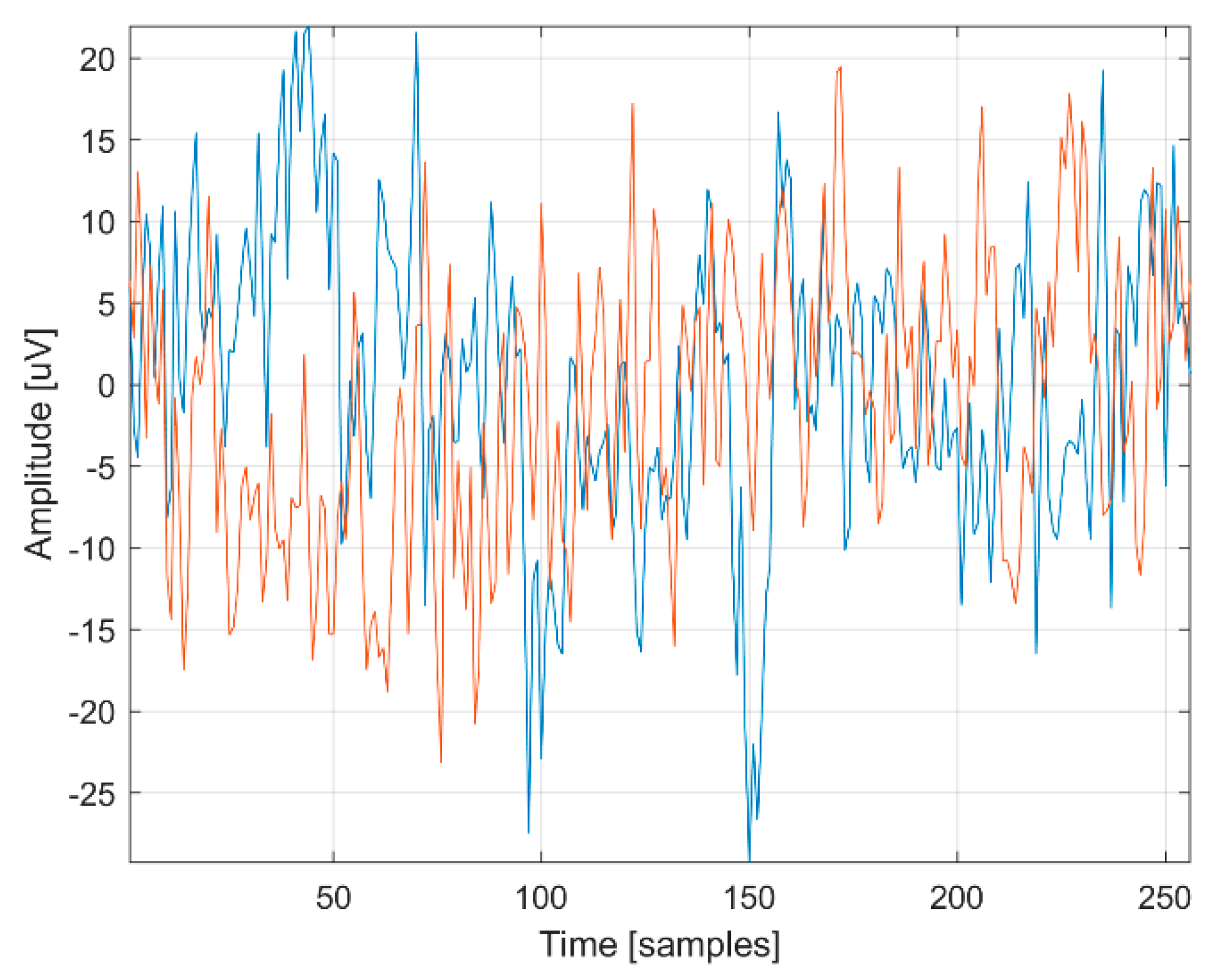
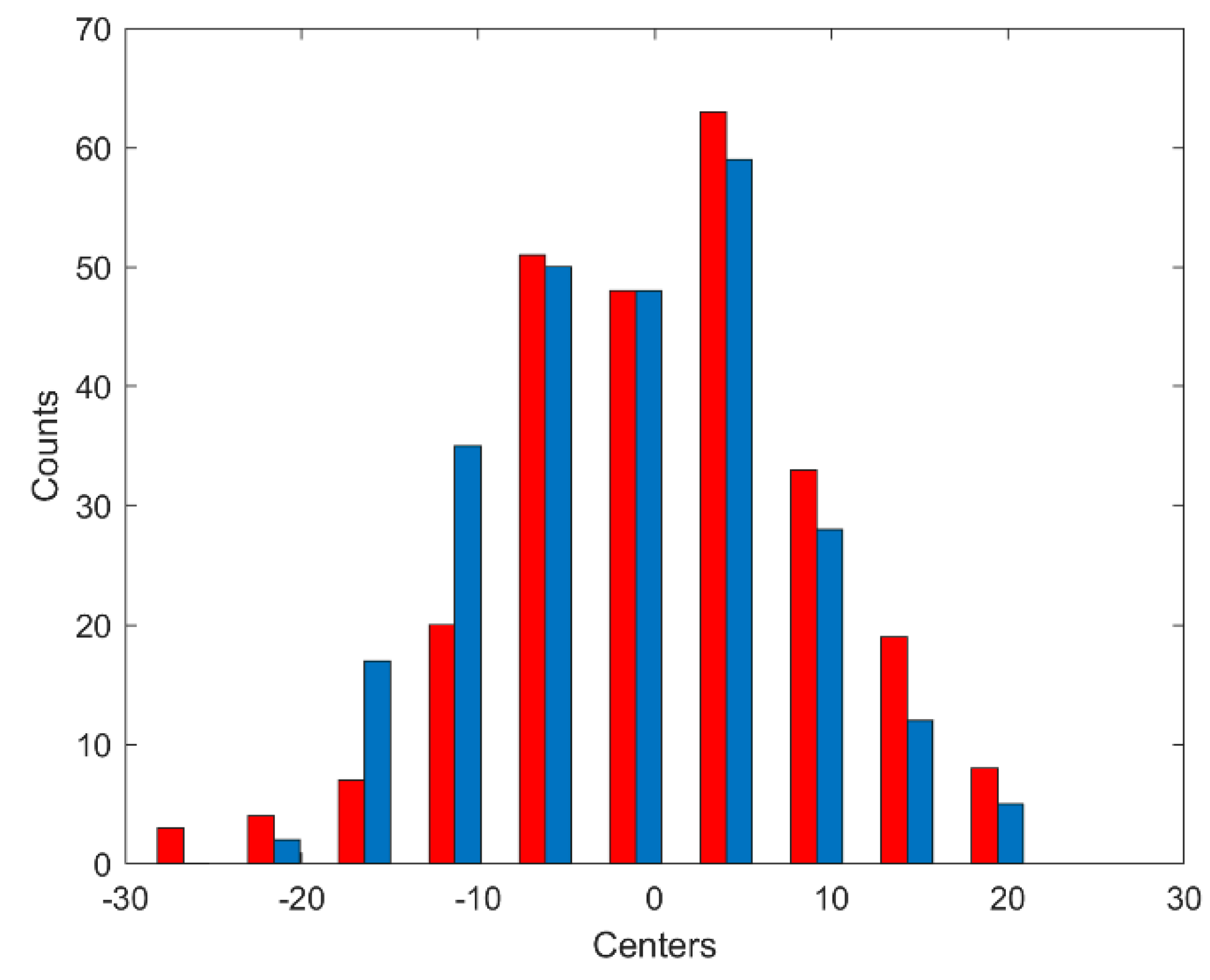
3.1. Data Augmentation

The method of data augmentation applied by us is based on the spectral analysis of the EEG signal. First, the spectral representation of EEG signals is built on the basis of previously recorded signals for stimulations with frequencies 5, 6, 7, and 8 Hz. The data augmentation procedure for each of the EEG signal channels is independent. The S signal recorded for each electrode is split into 1 s S_m windows. For the data recorded in the experiment, the sampling frequency is fs = 256 Hz. A window width of N = 256 samples was used, and the window was shifted with a small overlap of o = 10 samples. This made it possible to create a large number of M time windows. Then, for each S_m window, a spectral analysis was performed using discrete Fourier transform (DFT) [40]:

$$X_k={\sum }_{n=0}^{N-1}{(S_m)}_n{e}^{-\frac{i2\pi }{N}kn}$$

(1)

The spectral analysis enables the determination of the amplitudes of individual frequencies, which range from 0 to fs/2 Hz. The number of samples, N = 256, allowed for the acquisition of a frequency resolution of the signal equal to 1 Hz. As a result of the DFT analysis, we obtained the sets P_k = {$X_{k1}, X_{k2}, X_{k3}, \dots ,X_{kM}$} representing the amplitude values for the frequencies k = 0… fs/2 Hz. The P_k sets were used to generate new EEG signals. The augmentation algorithm enables the creation of a new artificial EEG signal with any number of L samples. The algorithm to create an artificial EEG signal is as follows:

1.

Create a new zero-time vector S_a of length L. This vector corresponds to the newly generated EEG signal for time samples from 0 to L × T − T (with step T).

2.

In a loop, for each value of frequency k = 0 to fs/2, perform the following:

a.

Choose an A_r value randomly from the range 〈−0.82; 0.82〉,

b.

Choose a φ_r value randomly from the range 〈−2$\pi ;2\pi$〉

c.

Choose a P_kr element randomly from the P_k set

d.

Update vector S_a according to the formula:

$$S_a=S_a+\left(P_{kr}+A_r\right)\sin \left(2\pi kt+{\phi }_r\right),$$

where t is a vector of time samples

3.

Add a vector R of length L to the vector Sa containing values chosen randomly from the range –ε to ε, where $\epsilon$ = 〈−1.84 × 10⁻⁸; 1.84 × 10⁻⁸〉

The result is a vector S_a corresponding to the newly generated EEG signal. Particular attention should be paid to the ranges from which the values A_r, φ_r, and $\epsilon$ are to be chosen. The typical values of the parameters were selected based on observations and were A_r = 〈−0.82; 0.82〉, φ_r = 〈−2$\pi ;2\pi$〉, and $\epsilon$= 〈−1.84 × 10⁻⁸; 1.84 × 10⁻⁸〉, respectively.

To obtain the augmented signal, the first 20 s of the recorded real EEG signals were used. As a result of data augmentation, we obtained 90,000 examples per class for each user (S01–S05), totaling 360,000 examples. Out of these, 10% were designated as validation data. Consequently, the CNN training set comprised 324,000 examples, while the validation set included 36,000 examples. Only the generated data were utilized for training the CNN. However, to evaluate the network’s performance, the last 10 s of the real recorded EEG signals were used. The method itself does not limit the number of examples that can be generated. From several hundred real EEG examples, it is possible to generate several thousand artificial examples. The morphology of the generated EEG signals is distinct, exhibiting completely new signal characteristics in the time domain. Nevertheless, the generated EEG signal maintains the same statistical parameters as the real one. Moreover, the spectrum of the generated signal closely resembles that of the real one. An illustration of one second of the real EEG signal (in blue) and the generated signal (in red) is presented in Figure 2. Figure 3 displays a histogram comparing samples of one second from the real EEG signal (in blue) and the generated signal (in red), highlighting their strong similarity. The spectra of the real EEG signal (in blue) and the generated one (in red) are depicted in Figure 4.

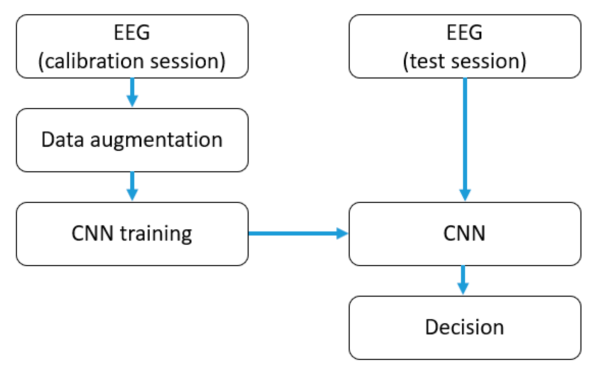
3.2. Convolutional Neural Network

The operation of CNNs is based on convolutional filters. When a signal passes through these filters, it is transformed into a vast array of features that are then classified by a fully connected layer. In the search for the optimal CNN architecture, the impact of varying the number of convolutional layers (ranging from 2 to 5) was examined. Additionally, the effect of the number of filters with values of 2, 4, 8, 16, 32, 64, 128, and 256 was evaluated. Subsequently, the influence of different filter sizes—2, 4, 8, 16, 32, and 64—was investigated. The selection of the network structure was derived from an automated search for the optimal combinations of layer count, filter count, and filter size. During our research, we did not consider the impact of the dropout layer on the CNN training process. During the selection of the best parameters, different optimizer algorithms (ADAM, SGD) and a range of values for InitialLearnRate (0.0001, 0.001, 0.01) and L2Regularization (0.01, 0.001, 0.0001) were evaluated. The search for the optimal combination of network structure and learning parameters spanned several days. The best network structure and parameters were determined based on the classification accuracy obtained for the validation data. The accuracies for the validation set for the considered structures ranged on average for all users from 0.65 to 0.72. The best results were achieved for the CNN network structure, which consisted of four convolutional layers, applying a ReLU activation function after each. The final convolutional layer, along with the subsequent ReLU layer, consists of 128 filters, resulting in a considerable number of features fed into the SoftMax classifier. The ADAM optimizer [37] was employed to train the CNN network, with an InitialLearnRate set at 0.001. Training was conducted over a maximum of 50 epochs, with a MiniBatchSize of 128 and an L2Regularization factor of 0.0001. The architecture of the CNN used in this study is detailed in

Table 1. CNN structure.

No.	Name of Layer	Parameters
1	Input Layer	256 × 3 × 1 signals with zero-center normalization
2	Convolution_1	32 filters of size 8 × 3 with stride [1 1] and padding ‘same’
3	Batch Normalization_1	Batch normalization with 32 channels
4	ReLU_1	ReLU
5	Convolution_2	64 filters of size 16 × 3 with stride [1 1] and padding
6	Batch Normalization_2	Batch normalization with 64 channels
7	ReLU_2	ReLU
8	Convolution_3	128 filters of size 32 × 1 with stride [1 1] and padding
9	Batch Normalization_3	Batch normalization with 128 channels
10	ReLU_3	ReLU
11	Convolution_4	128 filters of size 64 × 1 with stride [1 1] and padding
12	Batch Normalization_4	Batch normalization with 128 channels
13	ReLU_4	ReLU
14	Fully Connected	4 fully connected layer
15	Softmax	Softmax
16	Classification Output	Crossentropyex

. During the training of the network, the learning curve and error for the validation data were observed. No signs of overfitting in the CNN were noticed.

To train a CNN, a large number of training examples are needed. During training, we utilized a dataset obtained through the proposed augmentation method. However, for testing the performance of the CNN, we employed EEG signals recorded during the test session. The schematic for CNN application is presented in Figure 5. In the Supplementary Materials, there is the source code of our developed method for EEG data augmentation, as well as the code for the implementation of a CNN network that enables the classification of SSVEP.

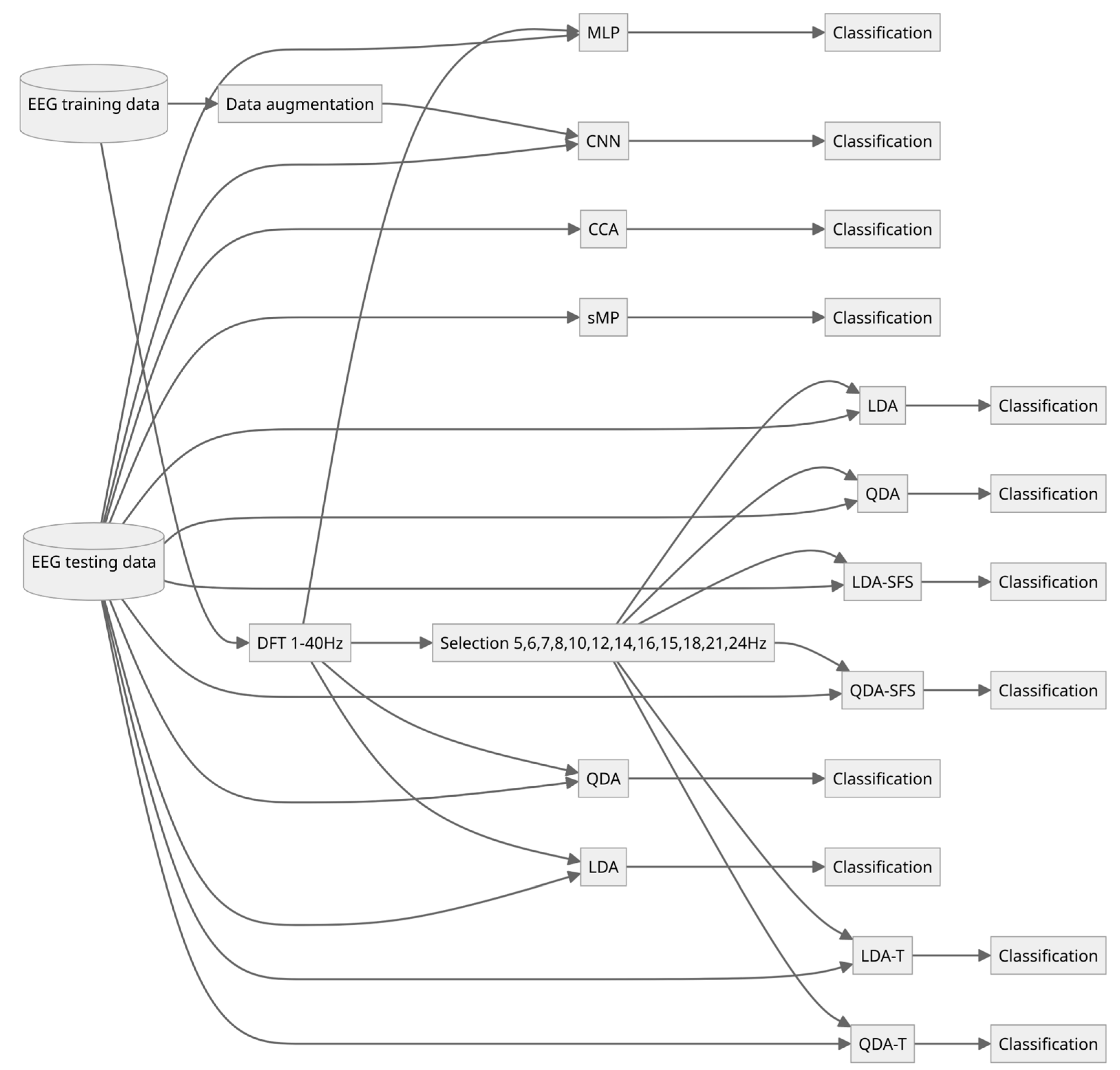
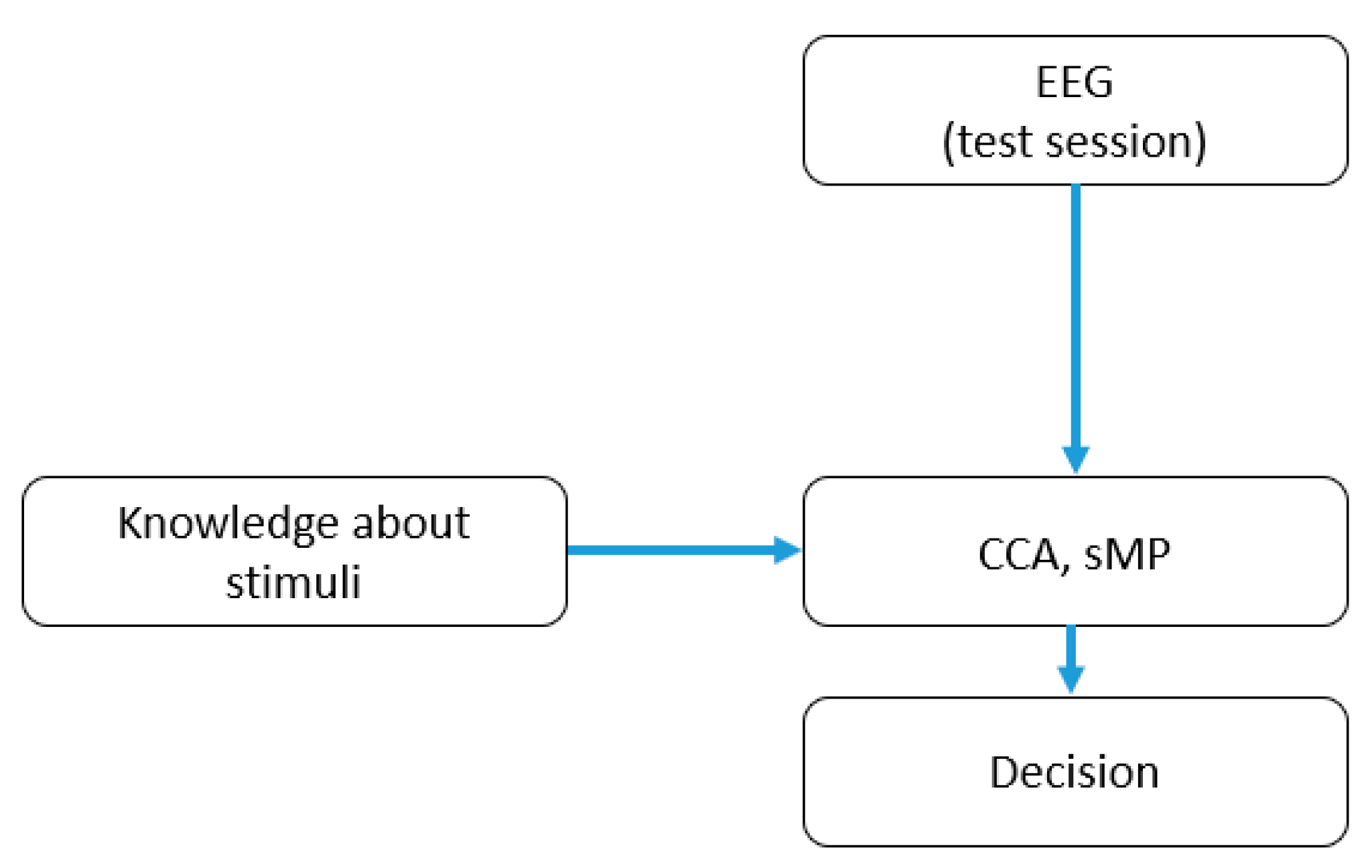
3.3. Classical SSVEP Detection Methods

The proposed CNN algorithm has been compared with a number of classical methods traditionally used for SSVEP detection. The concepts of utilizing classical and dedicated algorithms for SSVEP detection are illustrated in Figure 6 and Figure 7. Figure 6 demonstrates the application of typical machine learning methods, employing classifiers such as LDA, QDA, SVM, or MLP. The initial step involves training the classifier with data from a calibration session. Only after this step can the test data be classified. The classification process begins with the extraction of features from the EEG signal, followed by the selection of the most effective features. Figure 7 delineates the application of typical dedicated methods (such as CCA and sMP) for analyzing SSVEP. These methods do not necessitate a training session, but they do require knowledge of the frequencies of the stimuli. The aim is to find base signals that most closely correspond to stimuli at frequencies of 5 Hz, 6 Hz, 7 Hz, and 8 Hz. Canonical correlation analysis (CCA) seeks a linear combination between EEG signals and sinusoidal signals at the stimulation frequency and its harmonics. The frequency sought is the one for which the maximum correlation between EEG signals and sinusoidal signals, either at the stimulation frequency or its harmonics, is observed to be the largest [41]. Another method tailored for SSVEP detection is the sMP algorithm, which is derived from the well-known matching pursuit (MP) algorithm. However, the set of base functions in sMP is drastically narrowed down to sinusoidal signals at frequencies specifically chosen for visual stimulation.

Traditional machine learning methods require a feature extraction stage. Frequency analysis is often used to extract features from the EEG signal to detect SSVEP [42]. This is because, during user stimulation with frequency k, we expect an increased amplitude of the EEG signal in the visual cortex for the stimulation frequency k and its harmonics 2k, 3k. In our experiments, feature extraction was performed using DFT analysis. The spectrum was calculated from each second of the EEG signal, with a frequency resolution of 1 Hz. Such resolution should be sufficient to distinguish between the SSVEPs at stimulating frequencies of 5, 6, 7, and 8 Hz.

Feature vectors were constructed for each channel, corresponding to one of the two cases:

1.

All frequencies between 1 and 40 Hz were extracted.

2.

Only the frequencies of possible stimulations and their second and third harmonics were extracted. For the frequencies of 5, 6, 7, 8 Hz, these were, respectively: 5, 6, 7, 8, 10, 12, 14, 16, 15, 18, 21, and 24 Hz.

Feature extraction was performed for each channel separately. The use of three EEG signal channels triples the number of features. For case 1, there are 120 features, and for case 2, there are 48 features in total.

To ensure that the classifier is correctly trained using standard machine learning techniques, only the most useful features should be utilized, necessitating a feature selection stage. Various methods are employed to select the best features, with filter and wrapper approaches being the most common [43]. A typical filter method that is widely used is the t-test, which assumes a normal distribution of features. We implemented the absolute value two-sample t-test with a pooled variance estimate [44]. However, the t-test selection is typically designed for two groups, and in our case, there are four classes (5, 6, 7, and 8 Hz). Consequently, we adopted a strategy of selecting the best features for one class in contrast to all other combined classes. This approach allowed us to select the most distinctive features for the groups: 5 Hz versus (6, 7, 8 Hz), 6 Hz versus (5, 7, 8 Hz), 7 Hz versus (5, 6, 8 Hz), and 8 Hz versus (5, 6, 7 Hz). Subsequently, a subset of 14 features was chosen, which yielded the best classification performance for the training set. The number 14 was determined experimentally.

Unfortunately, feature selection methods do not always yield the best results because they do not consider the interdependencies between features [45]. A method that accounts for these types of dependencies is sequential forward selection (SFS) [46]. This method operates by selecting an initial feature, assessing the classification accuracy, and then incrementally adding the feature that most improves classification. For feature selection using SFS, the LDA and QDA classifiers were employed [47]. During the experiments, it was observed that the optimal number of features for achieving the highest classification accuracy was 25 for both LDA and QDA methods.

All experiments were conducted using MATLAB R2021a software on a computer equipped with an Intel Core i7-9800X processor, 128 GB of RAM, and an NVIDIA GeForce RTX 2080 Ti graphics card. The time required to execute various algorithms on the applied dataset, considering the established training parameters, varied significantly.

Table 2. Execution times of the individual algorithms.

Algorithm	Execution Time
Data set augmentation	12.115 s
CCA algorithm for classification (does not require training)	0.112 s
sMP algorithm for classification (does not require training)	0.311 s
Training the CNN for 50 epochs	145 min 8 s
Training the MLP	11.1 s
Training the LDA	14.3 s
Training the QDA	17.2 s
Training LDA with SFS/t-test feature selection	31.4 s/19.2 s
Training QDA with SFS/t-test feature selection	41.8 s/22.5 s

illustrates the time required to create the augmentation set, train the different classification methods, conduct feature selection, and train the CNN. However, it is important to note that both the CNN and MLP algorithms used a GPU for their calculations.

4. Results

Classification accuracy was used to evaluate the performance of individual classification methods. This measure is commonly used to assess classifiers and the effectiveness of BCI systems. The classification accuracy for each classifier was determined based on the last 10 s of real recorded EEG signals. During testing, 1 s windows overlapping by 0.5 s were employed, resulting in 72 windows for four stimulation frequency classes: 5, 6, 7, and 8 Hz.

Table 3. Comparison of the classification accuracies for the tested methods.

Method	CNN	CCA	sMP	MLP	QDA	LDA	QDA	LDA	QDA-SFS	LDA-SFS	QDA-T	LDA-T
Input	EEG raw			DFT 1–40 Hz	DFT 1–40 Hz	DFT 1–40 Hz	DFT 5 Hz, 6 Hz, 7 Hz, 8 Hz, 10 Hz, 12 Hz, 14 Hz, 16 Hz, 15 Hz, 18 Hz, 21 Hz, 24 Hz
Training the classifier on the generated data	Y	N	N	Y	Y	Y	N	N	N	N	N	N
Feature selection	-	-	-	-	-	-	-	-	SFS 25 features	SFS 25 features	t-test 14 features	t-test 14 features
Accuracy
User S01	0.81	0.75	0.58	0.62	0.62	0.75	0.65	0.66	0.62	0.63	0.68	0.76
User S02	0.88	0.54	0.51	0.61	0.61	0.59	0.56	0.40	0.48	0.47	0.61	0.50
User S03	0.42	0.40	0.29	0.30	0.27	0.31	0.23	0.33	0.26	0.33	0.18	0.22
User S04	0.75	0.54	0.54	0.70	0.65	0.68	0.58	0.65	0.56	0.65	0.59	0.56
User S05	0.75	0.63	0.61	0.63	0.63	0.65	0.62	0.58	0.61	0.59	0.66	0.62
Mean value	0.72	0.57	0.51	0.57	0.55	0.59	0.53	0.52	0.51	0.53	0.54	0.53
F1-score
User S01	0.79	0.59	0.46	0.51	0.48	0.59	0.56	0.53	0.51	0.51	0.55	0.60
User S02	0.87	0.41	0.33	0.49	0.50	0.48	0.45	0.28	0.31	0.33	0.48	0.33
User S03	0.29	0.30	0.19	0.18	0.18	0.23	0.15	0.24	0.12	0.25	0.11	0.14
User S04	0.60	0.40	0.42	0.56	0.54	0.55	0.46	0.55	0.43	0.54	0.47	0.45
User S05	0.60	0.51	0.50	0.50	0.52	0.51	0.50	0.46	0.50	0.48	0.53	0.49
Mean value	0.63	0.44	0.38	0.44	0.44	0.47	0.42	0.41	0.37	0.42	0.42	0.40

shows the accuracy and macro average F1-score results obtained for the individual classification methods on the test set. Macro average F1-score provides a balanced assessment of precision and sensitivity. In addition to the methods’ symbolic names (CNN, CCA, sMP, MLP, QDA, LDA, QDA-SFS, LDA-SFS, QDA-T, LDA-T), details about the data used at the classifiers’ input (EEG raw, DFT 1–40 Hz, DFT specific frequencies) and selection methods (SFS with 25 features, t-test with 14 features) are included. The table also indicates whether data augmentation was used for training (Y) or if it was the first 20 s of the recorded EEG signal (N).

The highest mean classification accuracy was achieved with the CNN at 0.72. A lower average accuracy of 0.57 was observed for both CCA and MLP. The sMP method yielded slightly inferior results, with an average classification accuracy of 0.51. Standard machine learning methods that employ spectral features and feature selection achieved classification accuracies ranging from 0.51 to 0.54. It is important to note that the classification pertained to 1 s windows across four classes. The random operation of a four-class classifier would result in a classification accuracy of 0.25. Therefore, it can be concluded that the methods under consideration deliver satisfactory results that are practically applicable. Attention should also be given to the variations in classifier accuracies among individual users. These differences can be attributed to the psychophysical characteristics of the person being tested and are a normal phenomenon. Additionally, some individuals are more naturally inclined to generate SSVEP responses to visual stimuli. To determine if the comparison of classification algorithms across five subjects (S01–S05) is reliable, statistical tests were conducted. Given the small sample size and the uncertain distribution of results, the non-parametric Wilcoxon–Mann–Whitney test was utilized [48]. p-values were calculated from a two-sided Wilcoxon signed-rank test. The classification accuracy results for the CNN method compared with other methods used by us (QDA, LDA, QDA-SFS, LDA-SFS, QDA-T, LDA-T, CCA and sMP) were found to be statistically significant at p = 0.0625. The improved classification accuracy of the CNN network may be due to its ability to automatically generate features. In contrast, other algorithms—whether specialized for SSVEP interfaces (like CCA and sMP) or standard machine learning methods (such as QDA, LDA, QDA-SFS, LDA-SFS, QDA-T, LDA-T)—relied on features derived from frequency analysis.

Table 3 presents the calculated F1-scores for various SSVEP potential classification methods. Among these, the CNN method attains the highest average F1-score of 0.63. Other methods, including CCA, MLP, QDA, and LDA, exhibit comparable results, with their average F1-scores ranging approximately from 0.44 to 0.47. This range indicates a moderate level of effectiveness for these techniques in SSVEPs classification. The sMP method recorded the lowest F1-score at 0.38, suggesting its comparatively limited utility. Meanwhile, the QDA and LDA methods, after incorporating SFS feature selection and the t-test, achieved F1-scores between 0.37 and 0.42. Overall, these findings imply that the CNN method is the most effective for SSVEP classification, whereas the other techniques demonstrate similar yet generally lower levels of effectiveness.

Future research should consider expanding the training dataset with EEG recordings from a greater number of individuals and employing different methods of stimulation, as well as various EEG signal acquisition systems.

5. Discussion

The results obtained can be converted into the information transfer rate (ITR), which are commonly used to compare brain–computer interface (BCI) systems.

Table 4. ITR comparison for classifiers [bit/min].

Subject	CNN	CCA
S01	59.8	47.5
S02	76.8	16.5
S03	5.95	4.6
S04	47.5	16.5
S05	47.5	27.7
Mean	42.0	19.9

compares the ITR results for individual users using both the CCA and CNN methods. The calculations reveal significant variations in the practical usability of the BCI interface among different individuals. It is important to note that the ITR was calculated based on the classification of one second continuous EEG signal segments. The decision-making time and classification accuracy substantially influence the information transfer rate. In practice, the actual ITR would be lower than the estimated values. Nonetheless, we can approximate the disparity in ITR by comparing the CNN and CCA methods for EEG signal classification. The largest difference, favoring the CNN method, is observed for user S02, at approximately 60.3 bits per minute, and the smallest for user S03, at 1.3 bits per minute.

It is important to consider that the analyses were conducted on SSVEP signals recorded under specific conditions and with individuals who had no previous experience with SSVEP interfaces, utilizing only three EEG signal electrodes. Various types of amplifiers, stimulation methods (such as stimulus brightness and LED size), and numbers of stimuli have been employed for recording SSVEP signals in the literature, complicating the comparison of classification results and ITR values across studies. In publication [38], EEG signals recorded using 8 channels and 12 stimulations were utilized, and the FB-EEGNet algorithm applied for classification yielded an ITR of 70.45 bits/min. In publication [49], a method based on task-related component analysis (TRCA) and an extended method based on canonical correlation analysis (CCA) for a 40-class SSVEP were implemented, with the online BCI speller achieving an average ITR of 325.33 ± 38.17 bits/min. Lastly, in publication [50], EEG data were recorded from 32 active electrodes, and by employing a spatially-coded BCI, the classification method reached an ITR of 31 ± 17 bits/min in novice users completing the task for the first time.

CNN delivers significantly better results for classification accuracy compared to other methods. During CNN training, filter weights are optimized to select useful features. The number of features processed through the fully connected layer is considerable: 128 filters × 3 EEG channels × 256 features per filter. This exceeds the number of features derived from selecting the 1–40 Hz frequency band, which is common in other methods. However, interpreting the function of these filters can be challenging. We can visualize the effects of these filters on the signals. Figure 8 displays a one second segment of the EEG signal from the O1 channel during a 5 Hz stimulus. Figure 9 illustrates the same signal after processing through a chosen filter from the fourth convolutional layer. Additionally, the spectra of these signals are shown, allowing for the analysis of the filter’s effect. In Figure 8, the original input signal to the filter has a broad frequency spectrum, but frequencies at 5 Hz, 10 Hz, and 15 Hz are not readily distinguishable. In contrast, Figure 9 reveals that the output signal from the filter predominantly features frequencies around 5, 10, and 15 Hz, which correspond to the stimulation frequency and its harmonics. Therefore, the signal post-filtering contains frequencies potentially beneficial for the classification of SSVEPs.

Several studies on CNNs indicate that the network is more robust to artifacts [51,52]. To determine whether the CNN approach is more effective in classifying SSVEPs with artifacts, we introduced Gaussian noise into the test signal. Gaussian noise closely approximates EMG artifacts resulting from muscular activities like jaw clenching, tongue movement, and swallowing [53]. We then attempted to classify sections of the noisy EEG signals for stimuli at 5, 6, 7, and 8 Hz. The classification accuracies for the CNN and CCA methods are listed in

Table 5. Comparison of classification accuracy for a noisy signal.

	EEG Signal (Std)	Noise (Std)	CNN	CCA
I	EEG (0.87 × 10−5)	-	0.81	0.75
II	EEG (0.87 × 10−5)	5.99 × 10−6	0.69	0.54
III	EEG (0.87 × 10−5)	1.60 × 10−5	0.59	0.45

. Case I presents the classification accuracies (0.81 for CNN and 0.75 for CCA) obtained with the originally recorded EEG signal, which had a standard deviation of 0.87 × 10⁻⁵. In Case II, Gaussian noise was added to the EEG signal with a standard deviation of 5.99 × 10⁻⁶, leading to a decrease in classification accuracy (0.69 for CNN and 0.54 for CCA). For Case III, the noise standard deviation was significantly increased to 1.60 × 10⁻⁵, which resulted in a further reduction in classification accuracy to 0.59 for CNN and 0.45 for CCA.

The augmentation of EEG data using the proposed method proved to be effective for SSVEP. This technique enables the creation of any number of training examples. However, the data augmentation method does not account for inter-channel relationships. If there are significant dependencies between channels O₁, O₂, and O_z—related to phase, frequencies, or amplitudes, for instance—the method may not generate accurate data for network training. Therefore, caution is advised when applying this technique to other potentials used in BCI, such as P300 or ERD/ERS.

The results we obtained align with those of other researchers who have applied CNN and deep learning to classification tasks in BCI systems. The experiment detailed in [54] involved nine flicker stimuli of different frequencies, and a CNN-based multitarget rapid classification method was constructed for nine classification tasks. The average accuracy of AR-BCI using the CNN model at a 1 s stimulus duration was about 81.83%. In [55], to enhance the classification accuracy of SSVEP signals during movement, SSVEP data were collected from five targets moving at speeds of 0 km/h, 2.5 km/h, and 5 km/h. A convolutional neural network (CNN) was developed to discern the relationship between the EEG signal and the pattern corresponding to each stimulus frequency. The proposed method outperformed traditional methods (i.e., CCA, FBCCA, and SVM) at all speeds, with CNN accuracies of 86.08%, 71.53%, and 60.63% from the lowest to highest walking speeds, respectively. In [26], the use of 64 channels yielded excellent results; however, when reduced to three channels, the classification accuracy was approximately 51% and 42% for sets of EEG signals. In [56], a BCI was utilized in an online experiment to spell the word ‘SPELLER’ using a 2 s time window. The system attained an average accuracy of 97.4% and an information transfer rate of 49 bpm, demonstrating the practicality and feasibility of implementing a reliable single-channel SSVEP-based speller using a 1D CNN. The study in [57] introduced a filter bank convolutional neural network (FBCNN) approach to optimize SSVEP classification. Three filters, each covering a harmonic of the SSVEP signals, were used to extract and differentiate the relevant components, with their information transformed into the frequency domain. Experimental results indicated that FBCNN enhances the performance of CNN-based SSVEP classification methods and holds significant potential for SSVEP-based BCIs. FBCNN results were approximately 2% better than those of traditional CNNs, though a wide dispersion of results was observed for both methods, varying by individual.

When attempting to implement CNNs in practical applications, certain challenges may arise. In our study, the classification time for 1 s of EEG signal was a rapid 3.7 ms. However, the training time required for the CNN poses a challenge. Here, transfer learning techniques could be vitally important. Utilizing transfer learning may necessitate adjustments to the signal sampling frequency and the number of network inputs, which must align with the number of recorded EEG channels. Additionally, it is crucial to retrain the network using a relatively large dataset.

We implemented the CNN proposed in article [26] to explore the potential of using transfer learning. The proposed network yields impressive results, achieving close to 98% accuracy for 1 s segments of the signal across all 64 channels. Its architecture reflects an understanding of EEG signal processing and analysis methods. The network was originally trained on data from 70 healthy individuals and 40 target characters, which flickered at frequencies ranging from 8 to 15.8 Hz in 0.2 Hz increments. This training used EEG data recorded at 250 Hz. We adapted this network structure for the data recorded from users S01–S05. The adaptation involved modifying the first and last layers of the CNN to accommodate three input channels (O₁, O₂, O_z) and four SSVEP frequencies (5 Hz, 6 Hz, 7 Hz, 8 Hz). We then retrained the network with the EEG training data, using the initial 20 s of the actual recorded EEG signal for S01–S05 users, after resampling the signals from 256 Hz to 250 Hz. Subsequently, we calculated the classification accuracy for SSVEP recognition on the training data (last 10 s) for each user. The classification results obtained for the adapted CNN [26] using transfer learning techniques are summarized in

Table 6. Comparison of classification accuracy for CNN [26].

Subject	CNN [26]	Our CNN	CCA
S01	0.85	0.81	0.75
S02	0.55	0.88	0.54
S03	0.30	0.42	0.40
S04	0.52	0.75	0.54
S05	0.82	0.75	0.63
Mean	0.61	0.72	0.57

. The table also includes comparative results from the CNN network that we developed as well as the CCA method.

The average recognition accuracy for the CNN [26] method is 61%, for the CCA method it is 57%, and for the CNN that we proposed, which includes data augmentation, it is 72%. These results suggest that the application of transfer learning techniques yields better outcomes than the use of standard machine learning methods like CCA. Nonetheless, our specialized approach achieved an 11% higher accuracy.

6. Conclusions

The results presented demonstrate that the use of CNN can significantly enhance the efficiency of SSVEP-based BCIs. Compared to traditional machine learning methods, CNN can provide up to 20% better results. This improvement leads to a substantially higher ITR and more effective BCI system operations. A CNN classifier trained for this purpose is more resistant to artifacts in the EEG signal than other SSVEP detection methods. The data augmentation method proposed for calibration sessions enables effective CNN training. Unfortunately, the use of CNN is not without practical limitations. One drawback is the extensive training time required, which may span several hours. Additionally, high classification accuracy is typically achieved only when the data from a specific individual’s calibration session are used for training. Furthermore, the same network structure cannot be directly applied to different databases. The CNN structure must be modified for signals recorded with varying equipment and different sampling frequencies.

References

1. Gu, X.; Cao, Z.; Jolfaei, A.; Xu, P.; Wu, D.; Jung, T.-P.; Lin, C.-T. EEG-Based Brain-Computer Interfaces (BCIs): A Survey of Recent Studies on Signal Sensing Technologies and Computational Intelligence Approaches and Their Applications. IEEE/ACM Trans. Comput. Biol. Bioinform. 2021, 18, 1645–1666. [Google Scholar] [CrossRef] [PubMed]
2. Li, M.; He, D.; Li, C.; Qi, S. Brain–Computer Interface Speller Based on Steady-State Visual Evoked Potential: A Review Focusing on the Stimulus Paradigm and Performance. Brain Sci. 2021, 11, 450. [Google Scholar] [CrossRef] [PubMed]
3. Norizadeh Cherloo, M.; Mijani, A.M.; Zhan, L.; Daliri, M.R. A Novel Multiclass-Based Framework for P300 Detection in BCI Matrix Speller: Temporal EEG Patterns of Non-Target Trials Vary Based on Their Position to Previous Target Stimuli. Eng. Appl. Artif. Intell. 2023, 123, 106381. [Google Scholar] [CrossRef]
4. Ramkumar, S.; Amutharaj, J.; Gayathri, N.; Mathupriya, S. A Review on Brain Computer Interface for Locked in State Patients. Mater. Today Proc. 2021. SSN 2214-7853. [Google Scholar] [CrossRef]
5. Choi, W.-S.; Yeom, H.-G. Studies to Overcome Brain–Computer Interface Challenges. Appl. Sci. 2022, 12, 2598. [Google Scholar] [CrossRef]
6. Abibullaev, B.; Kunanbayev, K.; Zollanvari, A. Subject-Independent Classification of P300 Event-Related Potentials Using a Small Number of Training Subjects. IEEE Trans. Hum.-Mach. Syst. 2022, 52, 843–854. [Google Scholar] [CrossRef]
7. Edlinger, G.; Allison, B.Z.; Guger, C. How Many People Can Use a BCI System? In Clinical Systems Neuroscience; Kansaku, K., Cohen, L.G., Birbaumer, N., Eds.; Springer: Tokyo, Japan, 2015; pp. 33–66. ISBN 978-4-431-55037-2. [Google Scholar]
8. Mu, J.; Grayden, D.B.; Tan, Y.; Oetomo, D. Comparison of Steady-State Visual Evoked Potential (SSVEP) with LCD vs. LED Stimulation. In Proceedings of the 2020 42nd Annual International Conference of the IEEE Engineering in Medicine Biology Society (EMBC), Montreal, QC, Canada, 20–24 July 2020; pp. 2946–2949. [Google Scholar]
9. Wang, J.; Bi, L.; Fei, W. Multitask-Oriented Brain-Controlled Intelligent Vehicle Based on Human–Machine Intelligence Integration. IEEE Trans. Syst. Man. Cybern. Syst. 2022, 53, 2510–2521. [Google Scholar] [CrossRef]
10. Waytowich, N.R.; Krusienski, D.J. Multiclass Steady-State Visual Evoked Potential Frequency Evaluation Using Chirp-Modulated Stimuli. IEEE Trans. Hum.-Mach. Syst. 2016, 46, 593–600. [Google Scholar] [CrossRef]
11. Lin, B.-S.; Wang, H.-A.; Huang, Y.-K.; Wang, Y.-L.; Lin, B.-S. Design of SSVEP Enhancement-Based Brain Computer Interface. IEEE Sens. J. 2021, 21, 14330–14338. [Google Scholar] [CrossRef]
12. Brennan, C.; McCullagh, P.; Lightbody, G.; Galway, L.; McClean, S.; Stawicki, P.; Gembler, F.; Volosyak, I.; Armstrong, E.; Thompson, E. Performance of a Steady-State Visual Evoked Potential and Eye Gaze Hybrid Brain-Computer Interface on Participants With and Without a Brain Injury. IEEE Trans. Hum.-Mach. Syst. 2020, 50, 277–286. [Google Scholar] [CrossRef]
13. Castillo, J.; Müller, S.; Caicedo, E.; Bastos, T. Feature Extraction Techniques Based on Power Spectrum for a SSVEP-BCI. In Proceedings of the 2014 IEEE 23rd International Symposium on Industrial Electronics (ISIE), Istanbul, Turkey, 1–4 June 2014; pp. 1051–1055. [Google Scholar]
14. Shao, X.; Lin, M. Filter Bank Temporally Local Canonical Correlation Analysis for Short Time Window SSVEPs Classification. Cogn. Neurodyn. 2020, 14, 689–696. [Google Scholar] [CrossRef] [PubMed]
15. Kołodziej, M.; Majkowski, A.; Rak, R.J. Simplified Matching Pursuit as a New Method for SSVEP Recognition. In Proceedings of the 2016 39th International Conference on Telecommunications and Signal Processing (TSP), Vienna, Austria, 27–29 June 2016; pp. 346–349. [Google Scholar]
16. Waytowich, N.R.; Faller, J.; Garcia, J.O.; Vettel, J.M.; Sajda, P. Unsupervised Adaptive Transfer Learning for Steady-State Visual Evoked Potential Brain-Computer Interfaces. In Proceedings of the 2016 IEEE International Conference on Systems, Man, and Cybernetics (SMC), Budapest, Hungary, 9–12 October 2016; pp. 004135–004140. [Google Scholar]
17. Müller-Putz, G.R.; Scherer, R.; Brauneis, C.; Pfurtscheller, G. Steady-State Visual Evoked Potential (SSVEP)-Based Communication: Impact of Harmonic Frequency Components. J. Neural Eng. 2005, 2, 123–130. [Google Scholar] [CrossRef] [PubMed]
18. Liu, Q.; Jiao, Y.; Miao, Y.; Zuo, C.; Wang, X.; Cichocki, A.; Jin, J. Efficient Representations of EEG Signals for SSVEP Frequency Recognition Based on Deep Multiset CCA. Neurocomputing 2020, 378, 36–44. [Google Scholar] [CrossRef]
19. Lahane, P.; Jagtap, J.; Inamdar, A.; Karne, N.; Dev, R. A Review of Recent Trends in EEG Based Brain-Computer Interface. In Proceedings of the 2019 International Conference on Computational Intelligence in Data Science (ICCIDS), Chennai, India, 21–23 February 2019; pp. 1–6. [Google Scholar]
20. Osowski, S.; Cichocki, A.; Lempitsky, V.; Poggio, T. Deep Learning: Theory and Practice. Bull. Pol. Acad. Sci. Tech. Sci. 2018, 66, 757–759. [Google Scholar]
21. Shen, C.; Nguyen, D.; Zhou, Z.; Jiang, S.B.; Dong, B.; Jia, X. An Introduction to Deep Learning in Medical Physics: Advantages, Potential, and Challenges. Phys. Med. Biol. 2020, 65, 05TR01. [Google Scholar] [CrossRef]
22. Voulodimos, A.; Doulamis, N.; Doulamis, A.; Protopapadakis, E. Deep Learning for Computer Vision: A Brief Review. Comput. Intell. Neurosci. 2018, 2018, e7068349. [Google Scholar] [CrossRef]
23. Israsena, P.; Pan-Ngum, S. A CNN-Based Deep Learning Approach for SSVEP Detection Targeting Binaural Ear-EEG. Front. Comput. Neurosci. 2022, 16, 868642. [Google Scholar] [CrossRef]
24. Kwak, N.-S.; Müller, K.-R.; Lee, S.-W. A Convolutional Neural Network for Steady State Visual Evoked Potential Classification under Ambulatory Environment. PLoS ONE 2017, 12, e0172578. [Google Scholar] [CrossRef]
25. Ma, P.; Dong, C.; Lin, R.; Ma, S.; Jia, T.; Chen, X.; Xiao, Z.; Qi, Y. A Classification Algorithm of an SSVEP Brain-Computer Interface Based on CCA Fusion Wavelet Coefficients. J. Neurosci. Methods 2022, 371, 109502. [Google Scholar] [CrossRef]
26. Guney, O.B.; Oblokulov, M.; Ozkan, H. A Deep Neural Network for SSVEP-Based Brain-Computer Interfaces. IEEE Trans. Biomed. Eng. 2022, 69, 932–944. [Google Scholar] [CrossRef]
27. Ravi, A.; Manuel, J.; Heydari, N.; Jiang, N. A Convolutional Neural Network for Enhancing the Detection of SSVEP in the Presence of Competing Stimuli. In Proceedings of the 2019 41st Annual International Conference of the IEEE Engineering in Medicine and Biology Society (EMBC), Berlin, Germany, 23–27 July 2019; pp. 6323–6326. [Google Scholar]
28. Waytowich, N.; Lawhern, V.J.; Garcia, J.O.; Cummings, J.; Faller, J.; Sajda, P.; Vettel, J.M. Compact Convolutional Neural Networks for Classification of Asynchronous Steady-State Visual Evoked Potentials. J. Neural Eng. 2018, 15, 066031. [Google Scholar] [CrossRef] [PubMed]
29. Li, Y.; Xiang, J.; Kesavadas, T. Convolutional Correlation Analysis for Enhancing the Performance of SSVEP-Based Brain-Computer Interface. IEEE Trans. Neural Syst. Rehabil. Eng. 2020, 28, 2681–2690. [Google Scholar] [CrossRef] [PubMed]
30. Ikeda, A.; Washizawa, Y. Steady-State Visual Evoked Potential Classification Using Complex Valued Convolutional Neural Networks. Sensors 2021, 21, 5309. [Google Scholar] [CrossRef] [PubMed]
31. Xing, J.; Qiu, S.; Ma, X.; Wu, C.; Li, J.; Wang, S.; He, H. A CNN-Based Comparing Network for the Detection of Steady-State Visual Evoked Potential Responses. Neurocomputing 2020, 403, 452–461. [Google Scholar] [CrossRef]
32. Xing, J.; Qiu, S.; Wu, C.; Ma, X.; Li, J.; He, H. A Comparing Network for the Classification of Steady-State Visual Evoked Potential Responses Based on Convolutional Neural Network. In Proceedings of the 2019 IEEE International Conference on Computational Intelligence and Virtual Environments for Measurement Systems and Applications (CIVEMSA), Tianjin, China, 14–16 June 2019; pp. 1–6. [Google Scholar]
33. Maharana, K.; Mondal, S.; Nemade, B. A Review: Data Pre-Processing and Data Augmentation Techniques. Glob. Transit. Proc. 2022, 3, 91–99. [Google Scholar] [CrossRef]
34. He, C.; Liu, J.; Zhu, Y.; Du, W. Data Augmentation for Deep Neural Networks Model in EEG Classification Task: A Review. Front. Hum. Neurosci. 2021, 15, 765525. [Google Scholar] [CrossRef] [PubMed]
35. Kalaganis, F.P.; Laskaris, N.A.; Chatzilari, E.; Nikolopoulos, S.; Kompatsiaris, I. A Data Augmentation Scheme for Geometric Deep Learning in Personalized Brain–Computer Interfaces. IEEE Access 2020, 8, 162218–162229. [Google Scholar] [CrossRef]
36. Wang, F.; Zhong, S.; Peng, J.; Jiang, J.; Liu, Y. Data Augmentation for EEG-Based Emotion Recognition with Deep Convolutional Neural Networks. In Proceedings of the MultiMedia Modeling; Schoeffmann, K., Chalidabhongse, T.H., Ngo, C.W., Aramvith, S., O’Connor, N.E., Ho, Y.-S., Gabbouj, M., Elgammal, A., Eds.; Springer International Publishing: Cham, Switzerland, 2018; pp. 82–93. [Google Scholar]
37. Chiang, K.-J.; Wei, C.-S.; Nakanishi, M.; Jung, T.-P. Boosting Template-Based SSVEP Decoding by Cross-Domain Transfer Learning. J. Neural Eng. 2021, 18, 016002. [Google Scholar] [CrossRef]
38. Yao, H.; Liu, K.; Deng, X.; Tang, X.; Yu, H. FB-EEGNet: A Fusion Neural Network across Multi-Stimulus for SSVEP Target Detection. J. Neurosci. Methods 2022, 379, 109674. [Google Scholar] [CrossRef]
39. Duart, X.; Quiles, E.; Suay, F.; Chio, N.; García, E.; Morant, F. Evaluating the Effect of Stimuli Color and Frequency on SSVEP. Sens. 2020, 21, 117. [Google Scholar] [CrossRef]
40. Hui, S.; Żak, S.H. Discrete Fourier Transform and Permutations. Bull. Pol. Acad. Sciences. Tech. Sci. 2019, 675, 130874. [Google Scholar] [CrossRef]
41. Bin, G.; Gao, X.; Yan, Z.; Hong, B.; Gao, S. An Online Multi-Channel SSVEP-Based Brain-Computer Interface Using a Canonical Correlation Analysis Method. J. Neural Eng. 2009, 6, 046002. [Google Scholar] [CrossRef] [PubMed]
42. Tanaka, T.; Zhang, C.; Higashi, H. SSVEP Frequency Detection Methods Considering Background EEG. In Proceedings of the The 6th International Conference on Soft Computing and Intelligent Systems, and The 13th International Symposium on Advanced Intelligence Systems, Kobe, Japan, 20–24 November 2012; pp. 1138–1143. [Google Scholar]
43. Jović, A.; Brkić, K.; Bogunović, N. A Review of Feature Selection Methods with Applications. In Proceedings of the 2015 38th International Convention on Information and Communication Technology, Electronics and Microelectronics (MIPRO), Opatija, Croatia, 25–29 May 2015; pp. 1200–1205. [Google Scholar]
44. Wang, M.; Liu, G. A Simple Two-Sample Bayesian t-Test for Hypothesis Testing. Am. Stat. 2016, 70, 195–201. [Google Scholar] [CrossRef]
45. Zhou, X.; Wang, J. Feature Selection for Image Classification Based on a New Ranking Criterion. J. Comput. Commun. 2015, 3, 74–79. [Google Scholar] [CrossRef]
46. Tahir, M.A.; Bouridane, A.; Kurugollu, F. Simultaneous Feature Selection and Feature Weighting Using Hybrid Tabu Search/K-Nearest Neighbor Classifier. Pattern Recognit. Lett. 2007, 28, 438–446. [Google Scholar] [CrossRef]
47. Lotte, F.; Bougrain, L.; Cichocki, A.; Clerc, M.; Congedo, M.; Rakotomamonjy, A.; Yger, F. A Review of Classification Algorithms for EEG-Based Brain–Computer Interfaces: A 10 Year Update. J. Neural Eng. 2018, 15, 031005. [Google Scholar] [CrossRef] [PubMed]
48. Howard, C.W.; Zou, G.; Morrow, S.A.; Fridman, S.; Racosta, J.M. Wilcoxon-Mann-Whitney Odds Ratio: A Statistical Measure for Ordinal Outcomes Such as EDSS. Mult. Scler. Relat. Disord. 2022, 59, 103516. [Google Scholar] [CrossRef]
49. Nakanishi, M.; Wang, Y.; Chen, X.; Wang, Y.-T.; Gao, X.; Jung, T.-P. Enhancing Detection of SSVEPs for a High-Speed Brain Speller Using Task-Related Component Analysis. IEEE Trans. Biomed. Eng. 2018, 65, 104–112. [Google Scholar] [CrossRef]
50. Maÿe, A.; Mutz, M.; Engel, A.K. Training the Spatially-Coded SSVEP BCI on the Fly. J. Neurosci. Methods 2022, 378, 109652. [Google Scholar] [CrossRef]
51. Kołodziej, M.; Majkowski, A.; Tarnowski, P.; Rak, R.J.; Rysz, A. A New Method of Cardiac Sympathetic Index Estimation Using a 1D-Convolutional Neural Network. Bull. Pol. Acad. Sciences. Tech. Sci. 2021, 69, 136921. [Google Scholar] [CrossRef]
52. Zhang, Q.; Zhou, D.; Zeng, X. HeartID: A Multiresolution Convolutional Neural Network for ECG-Based Biometric Human Identification in Smart Health Applications. IEEE Access 2017, 5, 11805–11816. [Google Scholar] [CrossRef]
53. Furui, A.; Hayashi, H.; Nakamura, G.; Chin, T.; Tsuji, T. An Artificial EMG Generation Model Based on Signal-Dependent Noise and Related Application to Motion Classification. PLoS ONE 2017, 12, e0180112. [Google Scholar] [CrossRef] [PubMed]
54. Zhao, X.; Du, Y.; Zhang, R. A CNN-Based Multi-Target Fast Classification Method for AR-SSVEP. Comput. Biol. Med. 2022, 141, 105042. [Google Scholar] [CrossRef] [PubMed]
55. Wu, C.; Qiu, S.; Xing, J.; He, H. A CNN-Based Compare Network for Classification of SSVEPs in Human Walking. In Proceedings of the 2020 42nd Annual International Conference of the IEEE Engineering in Medicine Biology Society (EMBC), Montreal, QC, Canada, 20–24 July 2020; pp. 2986–2990. [Google Scholar]
56. Nguyen, T.-H.; Chung, W.-Y. A Single-Channel SSVEP-Based BCI Speller Using Deep Learning. IEEE Access 2019, 7, 1752–1763. [Google Scholar] [CrossRef]
57. Zhao, D.; Wang, T.; Tian, Y.; Jiang, X. Filter Bank Convolutional Neural Network for SSVEP Classification. IEEE Access 2021, 9, 147129–147141. [Google Scholar] [CrossRef]
Figure 1. Diagram of the conducted research.
Applsci 13 13350 g001
Figure 2. Example of one second of the real EEG signal (blue) and the generated signal (red).
Applsci 13 13350 g002
Figure 3. Histogram of samples of one second of the real EEG signal (blue) and the generated signal (red).
Applsci 13 13350 g003
Figure 4. Spectrum of the real EEG signal (blue) and the generated signal (red).
Applsci 13 13350 g004
Figure 5. Schematic illustration of using a CNN to classify SSVEPs.
Applsci 13 13350 g005
Figure 6. Schematic illustration of using classical methods for SSVEP detection.
Applsci 13 13350 g006
Figure 7. Schematic illustration of using dedicated methods (CCA, sMP) for SSVEP detection.
Applsci 13 13350 g007
Figure 8. One second fragment of the EEG signal fed to the network input and the spectrum of this signal.
Applsci 13 13350 g008
Figure 9. One second fragment of the EEG signal after applying the exemplary convolutional filter (no 110) in the 4th layer and spectrum of this signal.
Applsci 13 13350 g009