Article

Cross-Condition Fault Diagnosis of an Aircraft Environmental Control System (ECS) by Transfer Learning

by
Lilin Jia
*,
Cordelia Mattuvarkuzhali Ezhilarasu
and
Ian K. Jennions
IVHM Centre, Cranfield University, Bedford MK43 0AL, UK
*
Author to whom correspondence should be addressed.
Appl. Sci. 2023, 13(24), 13120; https://doi.org/10.3390/app132413120
Submission received: 13 November 2023 / Revised: 5 December 2023 / Accepted: 7 December 2023 / Published: 9 December 2023

Abstract

:
Fault diagnosis models based on machine learning are often subjected to degradation in performance when dealing with data that are differently distributed than the training data. Such an occasion is common in reality because machines usually operate under various conditions. Transfer learning is a solution for the performance degradation of cross-condition fault diagnosis problems. This paper studies how transfer learning algorithms transfer component analysis (TCA) and joint distribution alignment (JDA) improve the cross-condition fault diagnosis accuracy of an aircraft environmental control system (ECS). Both methods work by transforming the source and target domain data into a feature space where their distributions are aligned to allow a uniform classifier to act accurately in both domains. This paper discovered that both TCA and JDA produce significantly more accurate results than traditional methods on target domains with unlabelled ECS data taken at different operating conditions than the source domain. Additionally, when dealing with unlabelled data from unknown conditions bearing a different composition of classes in the target domain, TCA is found to be more robust and accurate, generating an average predictive accuracy of 95.22%, which demonstrates the ability of transfer learning in solving similar problems in the real-world application of fault diagnosis.

1. Introduction

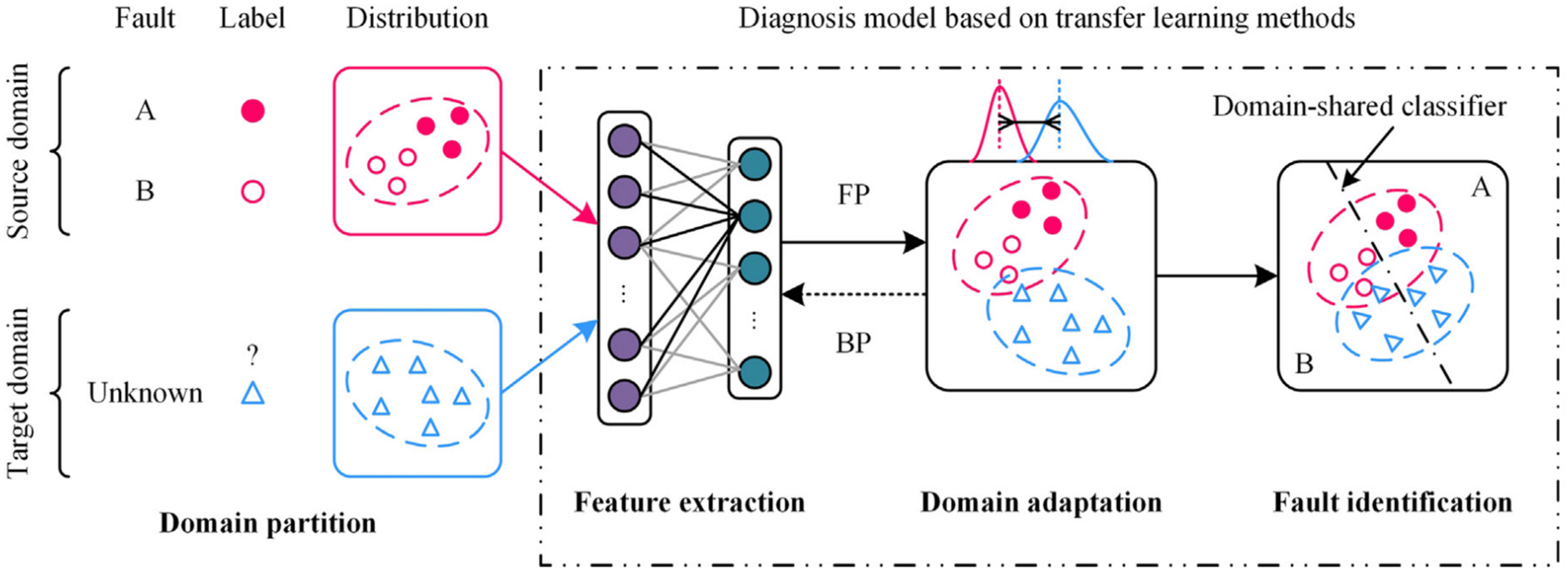
1.1. Cross-Condition Fault Diagnosis Using Transfer Learning

Fault diagnosis, the process of identifying faults and pinpointing the type of faults and root cause of the fault when they occur, plays a critical role in the monitoring of machines [1,2]. With advances in machine learning (ML), data-driven fault diagnosis has recently become a popular topic in academic research and industrial applications [3,4]. Empowered by the greater data analytical capacity of ML models when compared to traditional methods, data-driven fault diagnosis has demonstrated better diagnostic capacity when dealing with large datasets produced by machines with complex and integrated systems [5].
However, a common assumption in many data-driven fault diagnosis studies is that the data in the diagnosis task follow the same distribution as that used to train the ML models [6]. In reality, this assumption is difficult to achieve, because real machines operate under various operating conditions. For example, different loads and speeds might be imposed on bearings under different operating conditions, and the time-varying wind conditions would place wind turbine gearboxes under constantly varying operating conditions [7]. As a result, ML-based fault diagnosis algorithms would normally face data that have very different distributions from the data used in their initial training, and the distribution discrepancy between the training data and task data degrades the performance of ML-based fault diagnosis [8,9].
To overcome the performance degradation caused by distribution discrepancy and improve the accuracy of cross-domain fault diagnosis, transfer learning (TL) has been recognised as a promising solution. TL extracts knowledge from a source domain to boost the learning of ML models in a target domain and improve the accuracy of ML models in the target domain [10]. For cross-condition fault diagnosis problems, TL works by leveraging knowledge from a source domain with sufficient, labelled, balanced data with different distributions to improve the performance of ML models on target domain data [11]. There are abundant examples demonstrating the success of applying TL to cross-condition fault diagnosis in the existing literature.
Bearings and gearboxes are the most common specific applications for TL-based cross-condition fault diagnosis. Considering the cross-domain fault diagnosis between different loading conditions of bearings, He et al. [12] adopted a deep transfer learning method to transfer a convolutional neural network (CNN) trained in the source domain to the target domain data. Using CORrelation ALignment (CORAL) as the distance metric, the fully connected layers of the CNN in the source and target domains are aligned to ensure that the CNN trained by the source domain data under different conditions than the target domain data would perform accurately in the target domain [12]. To minimise the distribution discrepancy between the source and target domain data, Qian et al. [6] used joint distribution alignment (JDA) to align both marginal and conditional distributions so that the classifier trained with source domain data can act accurately on target domain data with different loading conditions. Tests on both bearing and gearbox datasets showed that their proposed TL-based method outperformed the comparison methods in terms of accuracy. Other applications include the cross-condition fault diagnosis for motors by Xiao et al. [13]. What is unique about this research is that, apart from considering different invariant working conditions, they included a condition-varying cycle for the test motor under the European Driving Cycle (NEDC). A CNN trained by source domain data was applied to the target domain data, and maximum mean discrepancy (MMD) was used to align the intermediate features to reduce the distribution discrepancy. Their TL-based fault diagnosis method achieved significantly higher accuracy when transferring from invariant working conditions to varying working conditions following NEDC.
Regarding aerospace topics, examples also exist for cross-condition fault diagnosis using TL. Li et al. [14] designed a TL-based algorithm for the fault diagnosis of aero-engine gas path data at different operating points. By unilaterally aligning the target domain to the source domain, the distribution discrepancy between the engine data at different operating points was minimised. Liu et al. [15] examined the cross-condition fault diagnosis of industrial gas turbines operating at different rotational speeds. Transfer of knowledge is achieved by reusing the structure and weight of the CNN trained by labelled source domain data in the target domain unlabelled data.
Although there have been numerous examples of applying TL in cross-condition fault diagnosis, most applications focus on component-level fault diagnosis rather than system-level problems. Hence, this work aims to discuss system-level cross-condition fault diagnosis using TL. Taking the aircraft environmental control system (ECS) as the system of interest, this system-level cross-condition fault diagnosis is generally more complicated than component-level studies, because more factors would affect the distribution discrepancy when the operating conditions change. For instance, when the operating conditions of a bearing change, only the speed, load, and wear condition affect the data, whereas, in an ECS, different operating conditions mean that a wide array of parameters from the ambient, bleed, and target conditions could all be different and contribute to the distribution discrepancy. In addition to more parameters, different interactions between the components are also expected under different operating conditions. Therefore, this work on how TL is applied to ECS cross-condition fault diagnosis would deepen the understanding of how TL facilitates cross-condition fault diagnosis at the system level.

1.2. Challenge of Cross-Condition Fault Diagnosis of Environmental Control System

The uniqueness of studying cross-condition fault diagnosis for ECS arises from the fact that, in real flights, the operating conditions of ECS frequently changes, which makes it nearly impossible to gather and label data under all possible operating conditions. Hence, this paper applies TL in fault diagnosis of target domains with unlabelled ECS data taken at unknown operating conditions. The fault diagnosis algorithm developed under this realistic setting will have significant value to design real-world fault diagnosis algorithm for ECS.
The rest of this paper is organised as follows. Section 2 introduces background information about the ECS, describes the data collection process, and provides a problem statement. Section 3 describes the methodology and the algorithm used in this study. Section 4 applies the method to ECS data under a specific transfer scenario and compares the results of a TL-based approach with those of non-TL approaches. Section 5 expands the transfer scenario to include both unknown operating conditions and different compositions of cases in the target domain, which tests the ability of the model to generalise. Section 6 tests and evaluates the TL-based approach with an alternative method to solve cross-domain fault diagnosis to further the understanding of the TL-based method. Finally, Section 7 concludes the paper.

2. Background

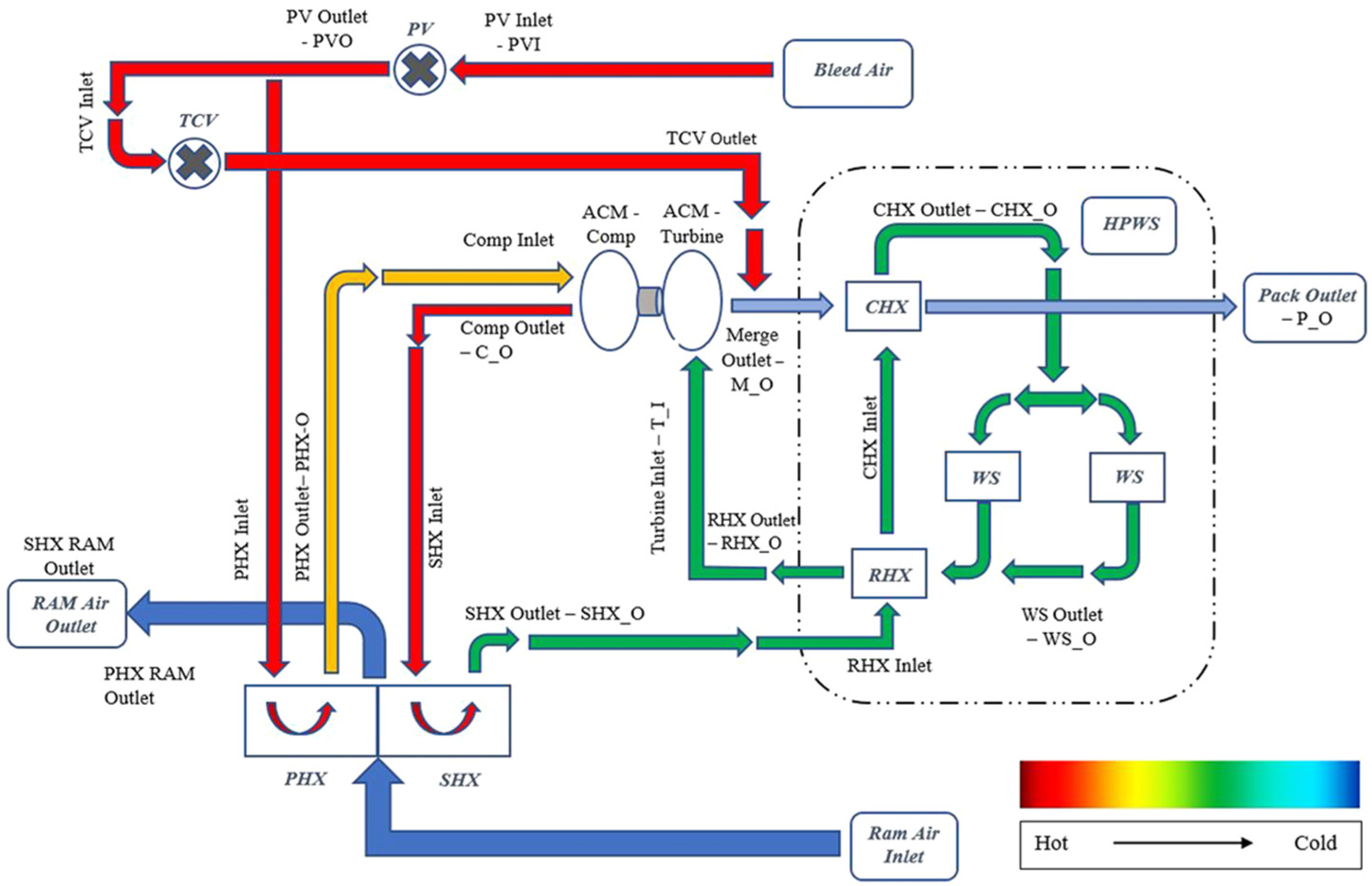
2.1. Environmental Control System Overview and Simulation Platform

The role of an ECS is to supply conditioned air to the aircraft cabin and cooling air to the avionics bay [16]. To ensure that the supplied air is at an appropriate temperature and humidity, Passenger Air Conditioners (PACK) are the primary subsystems within the ECS that condition air. A schematic of the PACK for a Boeing 737–800 is shown in Figure 1 [16], and a brief description of its working principles is given below.
The high-temperature and high-pressure air taken from the engine bleed first passes through the PACK Valve (PV), which controls the total mass flow rate into the system. A proportion of this hot air stream passes directly to the merge outlet through the Temperature Control Valve (TCV), while the rest passes through a cooling cycle and becomes a cold air stream. The PACK outlet temperature can be controlled by regulating the opening degree of the TCV, which regulates the proportion of the hot and cold air streams. The proportion of bleed air that passes through the cooling cycle first enters the Primary Heat Exchanger (PHX), where its temperature drops by transferring heat to the cold ram air. Next, its temperature and pressure are recovered through the compressor of the Air Cycle Machine (ACM) to allow a higher heat exchange rate and hence better effectiveness during the subsequent heat exchange in the Secondary Heat Exchanger (SHX), where it is cooled down again. The outlet air from the SHX then enters the High Pressure Water Separator (HPWS), where water is condensed and extracted before the air enters the turbine. The air expands through the ACM turbine, which drives the compressor, and its temperature and pressure are reduced. After merging with the hot stream at the TCV outlet and passing through the HPWS again, the air reaches the PACK outlet.
For ground operation, the PACK cycle works in the same manner, except that the bleed air comes from the Auxiliary Power Unit (APU) rather than the engines.
The PACK cycle described above can be simulated by Simscape Environmental Control System Simulation under All Conditions (SESAC) [17], an ECS simulation platform validated against actual data from Boeing 737–800 aircraft. The configuration of the PACK cycle in SESAC was identical to that of the Boeing 737–800 described above.
Five fault modes were simulated: ACM fault, PHX fault, SHX fault, TCV fault, and ram air intake (RI) blockage. Different degradation levels were simulated for each fault mode, as summarised in Table 1. The ACM fault is simulated by assigning degraded mechanical efficiency to the component, and the degradation degree in Table 1 corresponds to the percentage reduction in mechanical efficiency from the healthy-state. PHX and SHX faults were simulated by inputting the degraded heat exchanger effectiveness for PHX or SHX, representing both fouling and blockage in the heat exchangers [18]. The degradation degree for PHX and SHX in Table 1 corresponds to the percentage reduction in the heat exchanger effectiveness compared with healthy PHX and SHX values. RI blockage was also simulated at three levels, by simulating 25%, 50%, and 75% reductions in ram air mass flow rate compared to the commanded value. The TCV fault is simulated in a different way owing to the nature of the fault. While the TCV opening angle was found to be between 15° and 18° for the cases studied, faults can occur if the valve is jammed at a lower or higher angle than the commanded angle, resulting in an undershoot or overshoot, respectively. In the case of the undershoot, the TCV opening angle was fixed at 10°, and in the case of the overshoot, the TCV opening angle was fixed at 23°. Any fault with the HPWS is not considered as the simulation was carried out assuming no water in the bleed air.

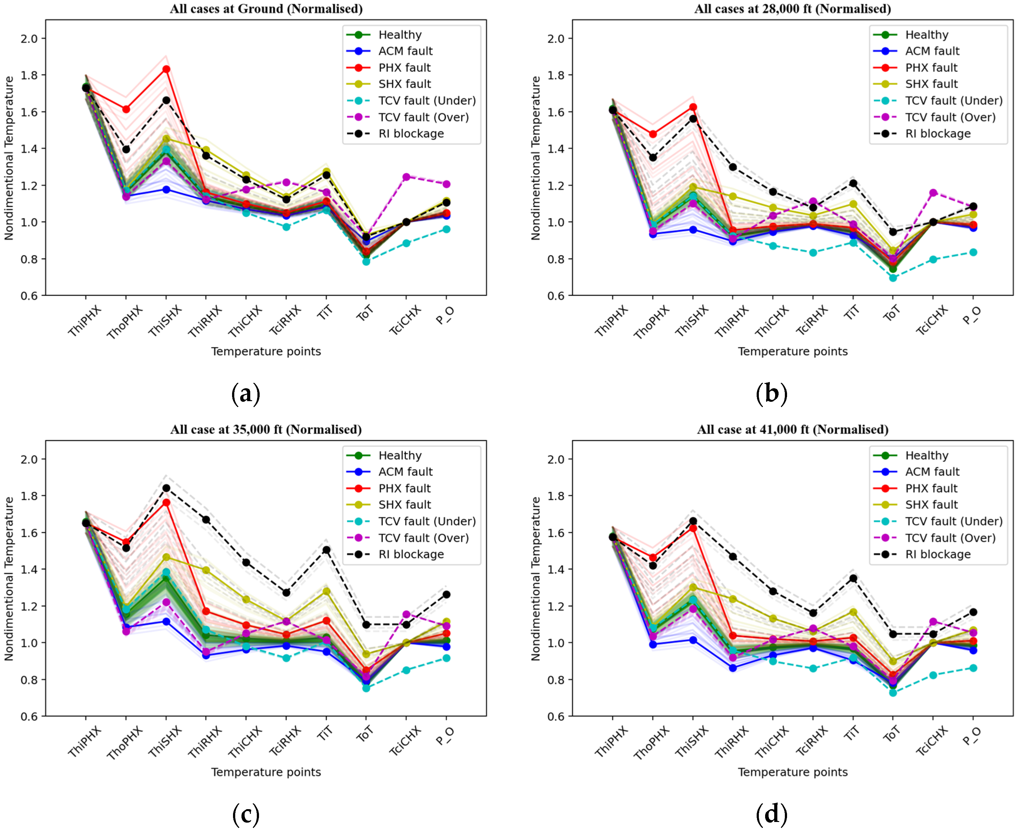
2.2. Data Collection and Processing

To produce data for this study, the SESAC code was run under four operating conditions, summarised in Table 2. Condition A represents a ground-running condition, and conditions B–D represent cruise conditions. Condition B (28k ft) corresponds to a typically low cruise altitude, and condition D (41k ft) to a typically high cruise altitude for a Boeing 737–800. All conditions and associated parameters were obtained from a dataset with the actual ECS data of a Boeing 737–800, so the parameters used represent real flight conditions. Under each condition, the main factors that determine the operation of the PACK are listed in Table 2, which includes the temperature and pressure from the engine bleed air, ram-air temperature, target temperature, and mass flow rate settings.
To incorporate real-life noise and uncertainties in the SESAC simulation results, the simulations were run with slightly perturbed parameters, in addition to runs with the original parameters. Specifically, a perturbation was imposed on the target temperature and target mass flow rate. The target temperature in each condition was set with values within a range of ±10 K from its mean value (i.e., a maximum of roughly 4% perturbation), and the target mass flow rate was set with values within a range ±0.02 kg s−1 from its mean value (a maximum of roughly 5% perturbation).
For each operating condition, 91 healthy-state cases were simulated and recorded, and 90 faulty-state cases were simulated and recorded, with 18 cases in each fault mode under various degradation severities. Among the temperature, pressure, and mass flow rate profiles, the temperature profile of the PACK was selected as the basis for developing its fault diagnosis algorithm, because it displays distinct patterns under different health states.
Before inputting data to the diagnosis algorithm, only one processing stage is conducted on the simulation results, which is normalising the temperature readings against the corresponding target temperature in each case, a boundary condition input in the simulations as the commanded temperature for PACK outlet. This was to alleviate the influence on the temperature profiles owing to the different target temperatures set in each case. Figure 2 shows the normalised simulation results of PACK temperature profiles under the four different operating conditions, plotted against temperature points proceeding from inlet to exit, aligned with the stations shown in Figure 1. For example, ThiPHX is the temperature at the inlet of the PHX. The different colours relate to the different health status of each component, with the baseline healthy condition being shown in green. The TCV fault is really only one fault with two states: undershoot or overshoot, as shown in Table 1. For clarity, one representative case per class is plotted, while other cases are shown in transparent lines.

2.3. Problem Statement

This study aims to develop a TL-based fault diagnosis algorithm, for the PACK model discussed, that leverages knowledge from a source domain with sufficient labelled data collected at one operating condition to accurately predict the health state labels for a target domain with no labelled data taken at a different operating condition than that of the source domain.
The problem represents a common real-life scenario in which, after training a fault diagnosis model with labelled data under known conditions, systems such as the ECS are likely to be operated under a vast variety of conditions, generating massive amounts of unlabelled data under new conditions that are not considered in the initial training stage. Because labelling new data under every new condition is expensive or even impossible, there is a practical need to develop a fault diagnosis algorithm that can handle unlabelled data under new operating conditions.

3. Methodology

3.1. Feature-Based TL: TCA and JDA

When operating conditions change, machines tend to produce data with different distributions, making traditional machine learning models, trained under previous conditions, inaccurate under new operating conditions [6]. Feature-based TL can correct such cross-condition distribution discrepancy by finding optimal mapping functions to map the source and target domain data into a common feature space, where their distribution discrepancy can be reduced [10,19]. A graphical description of feature-based TL is shown in Figure 3 [19,20]. Data from the source and target domains with different distributions are transformed into features in the feature space, where a distance metric could be applied to measure the discrepancy between the source and target domain features. This information then propagates back to the feature mapping stage to allow optimisation of the mapping functions with the aim of minimising the discrepancy between the source and target domain features in the feature space. Finally, the distributions of the source and target domain features are sufficiently aligned to allow a domain-invariant classifier to act accurately on both domains.
There are two types of distribution of source and target domain data, which feature-based TL can consider—marginal and conditional distributions [21]. The mathematical expression for the distributions will be introduced later in this section but the marginal distribution refers to the distribution of data regardless of the associated labels, whereas the conditional distribution is approximated and calculated as the distribution of data with a common label association.
Among the three major categories of TL approach in fault diagnosis, instance-based, feature-based, and parameter-based TL, the feature-based TL is determined to be the optimal approach for the problem of interest. The instance-based approach, which reweighs the source domain instances and uses them as auxiliary datasets for target domain problems, is not ideal, because identical conditional distribution is assumed for source and target domain [22]. The parameter-based TL, which reuses hyperparameters in pretrained models from source domain in target domain, is not chosen, since this approach may fail at significant distribution discrepancy [22].
The specific feature-based TL methods used in this work are transfer component analysis (TCA) and joint distribution alignment (JDA). Both algorithms are commonly studied feature-based TL algorithms, with successful application to bearings and gears, and other niche applications including spacecraft attitude systems, ball screws, and reciprocating compressors [19,23,24,25,26,27]. TCA and JDA have been commonly applied to fault diagnosis based on vibration data, but application has not been found on static signal data, such as the ECS data in this paper. It is worth exploring how TCA and JDA perform in the ECS dataset, because differences in the complex boundary conditions for ECS under different conditions is likely to lead to significant and unpredictable distribution discrepancies, which are particularly challenging for TL methods. Hence, this work applies TCA and JDA as the TL algorithm to attempt the cross-condition fault diagnosis problem for the PACK.
TCA and JDA follow similar mathematical operations to align the distribution discrepancy between the source and target domains. The difference between TCA and JDA is that while TCA only considers marginal distribution, JDA considers both marginal and conditional distribution alignment between the source and target domains [28]. More mathematical details of the two algorithms can be found in the original papers on TCA and JDA [21,29] but, to better understand how TCA and JDA reduce the cross-domain distribution discrepancy, the fundamental mathematical calculations used in TCA and JDA for the distribution discrepancy are described here.
Consider a labelled source domain D s = { x 1 , y 1 ,   x n s , y n s } , and an unlabelled target domain D t = x n s + 1 , , x n s + n t , where there are n s samples in the source domain, each with a symptom vector x of m dimensions and a corresponding health state label y , and there are n t samples in the target domain each with a symptom vector x of m dimensions. The source and target domains share the same m-dimensional feature space but different marginal and conditional probability distributions; that is, P s x s P t x t ,   Q s y s x s Q t y t x t . The data from the source and target domains were compiled into a data matrix X = [ x 1 , , x n ] R m × n , which maps to a feature space matrix Z = A T X through the transformation matrix A . The goal of TCA and JDA is to determine the optimal A that minimises the distribution discrepancy between the source and target domain cases in the feature space.
In TCA, the marginal distribution discrepancy is calculated by the following equations [21]:
1 n s i = 1 n s A T x i 1 n t j = n s + 1 n s + n t A T x j 2 = t r A T X M 0 X T A
M 0 i j = 1 n s n s , x i , x j D s 1 n t n t , x i , x j D t 1 n s n t , o t h e r w i s e
Similar to the calculation of the maximum mean discrepancy (MMD), the LHS of Equation (1) shows the calculation of the marginal distribution discrepancy, which can be interpreted as the vector norm of the difference between the mean source domain transformed feature vectors and the mean target domain transformed feature vectors. The LHS of Equation (1) is transformed into the RHS by introducing the MMD matrix M 0 , as shown in Equation (2).
In JDA, the conditional distributions considered, Q s y s x s and Q t y t x t are approximated by class-conditional distributions Q s x s y s and Q t x t y t instead. Considering the label space of C classes, c { 1 , , C } , the conditional distribution discrepancy, Q s x s y s = c and Q t x t y t = c , is calculated using the following equations [21]:
1 n s ( c ) x i D s ( c ) A T x i 1 n t ( c ) x j D t ( c ) A T x j 2 = t r A T X M c X T A
M C i j = 1 n s ( c ) n s ( c ) , x i , x j D s ( c ) 1 n t ( c ) n t ( c ) , x i , x j D t ( c ) 1 n s ( c ) n t ( c ) , x i D s c , x j D t ( c ) x j D s c , x i D t ( c ) 0 , o t h e r w i s e
Note that Equation (3) is structurally similar to Equation (1), with the major difference being that the distribution discrepancy is calculated for the source and target domain cases bearing the same label and then averaged over all labels. The RHS of Equation (3) is the equivalent expression as LHS of Equation (3) by introducing the MMD matrix involving class labels M c , as shown in Equation (4). A subtlety in this calculation is that, for unlabelled target domains, pseudo labels are used when computing the target domain conditional distribution, which are obtained by applying a classifier trained on the labelled source domain data to the unlabelled target domain data [21]. For this reason, to improve the final predictive accuracy, JDA follows an iterative process, where the predicted pseudo labels are supposed to become increasingly accurate as the conditional distribution calculation becomes more accurate through the iterations until convergence.
min A T XH X T A = I c = 0 C t r A T X M c X T A + λ A
Combining with principal component analysis (PCA), the overall optimisation equation for JDA is shown as Equation (5), where H is the centring matrix in PCA, and λ regulates the regularisation term to keep the optimisation well-defined [21]. TCA is a special case for C = 0 .
The JDA algorithm used in this study was obtained from [30]. As observed from running and examining the JDA algorithm, the first loop of the iterative process corresponds to a TCA operation, and from the second loop onwards, each loop corresponds to a JDA operation. Convergence was reached for all the scenarios tested before the 20th loop. Therefore, the TCA results reported are from the first loop, and the JDA results reported are from the 20th loop.

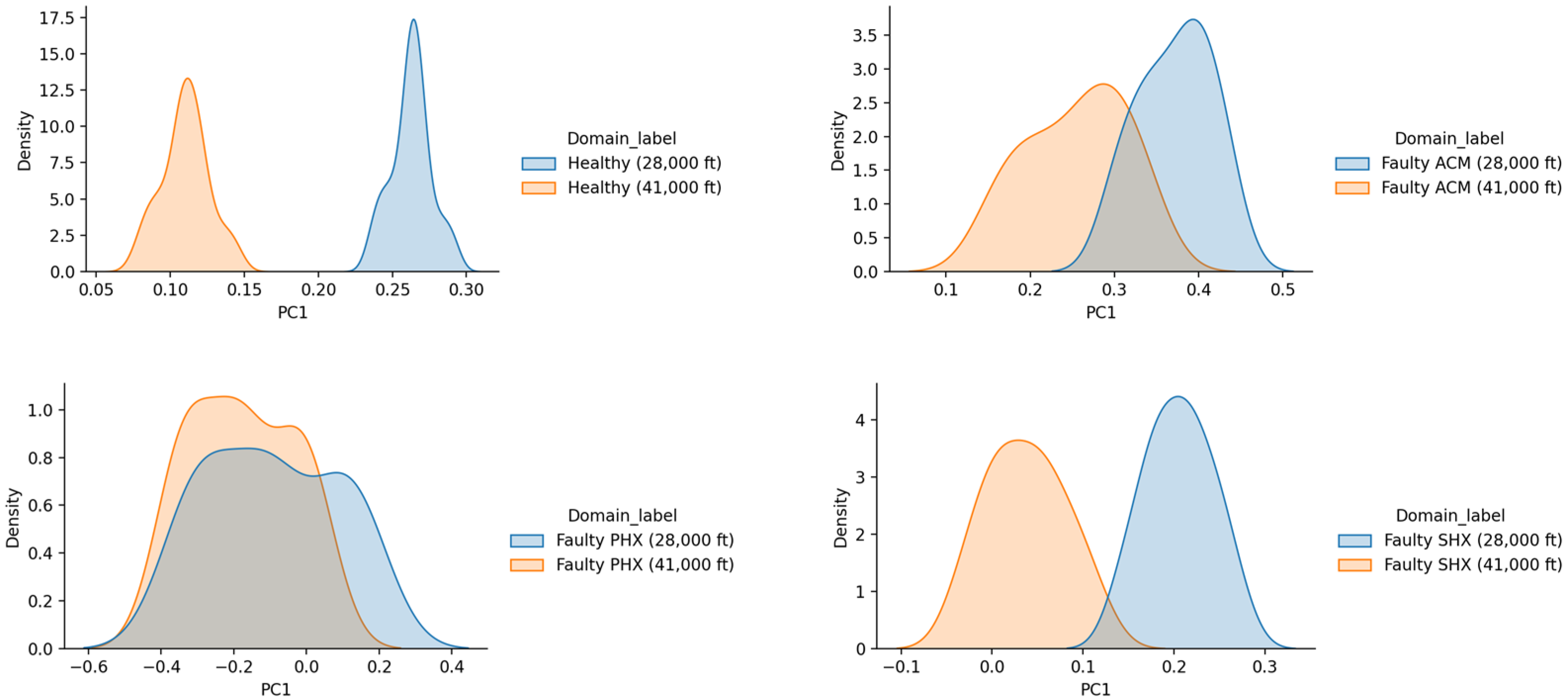
3.2. Visualising Marginal and Conditional Distribution Discrepancy

For the PACK data simulated in this study, both marginal and conditional distributions show significant discrepancy in the data taken under different operating conditions. To visualise this cross-domain distribution discrepancy, PCA is performed on the temperature profiles for the 28k ft and 41k ft cases. The distribution of the first principal components for the cases under these two conditions is plotted in Figure 4 and Figure 5.
As later sections will demonstrate, the discrepancy in the distribution of PACK simulation results under different operating conditions has been identified as the cause of misclassification. Therefore, TCA and JDA are potential techniques to help reduce the cross-domain distribution discrepancy and improve cross-domain diagnostic accuracy.

4. Result and Analysis

The ECS simulation data was obtained for the four operating conditions shown in Table 1. To develop a TL-based fault diagnostic algorithm, two of the conditions were arbitrarily selected as the source and target domains. A summary of the chosen conditions is presented in Table 3, with the source domain being taken at a low cruising altitude of 28k ft and consisted of both simulated PACK data and associated labels. The target domain was taken at the higher cruising altitude of 41k ft, which consisted of only simulated PACK data and no labels. The intention of choosing only one set of operating conditions as the source and target domain is so that the diagnostic algorithm developed in this transfer scenario can then be tested, in Section 5.1, for its ability to generalise when presented with data at new operating conditions to which the algorithm has not been exposed.

4.1. Non-TL Approach

To establish a baseline diagnostic accuracy for the TL-based approach, a diagnostic process without TL was first tested.
The non-TL approach consisted of two stages. The first stage aims at dimensionality reduction, and the technique chosen uses the minimal-redundancy-maximal-relevance (mRMR) criterion [31]. mRMR selects the most important features among all parameters in the PACK simulation data, ranking them from those with the highest relevance to the labels and the lowest redundancy with other features [31]. Compared to other dimensionality reduction techniques that map data onto a lower-dimensional space, the features selected by mRMR still carry physical significance, and hence, can be physically interpreted. In the second stage, a classifier is required to map each symptom vector (i.e., the vector of a PACK simulation case with features selected by mRMR) to a health state label. In this study, the k-nearest neighbour (k-NN) algorithm was chosen.
Because there is no label for the target domain data, k-NN cannot be trained by it. The only way to predict target domain labels is by training the k-NN with source domain labelled data and then directly applying the trained k-NN to predict labels in the target domain. In addition, to verify the training of the k-NN, 80% of the source domain data was used for training, and the other 20% was used for validation. After passing the training and validation steps, the k-NN classifier can be used on the target domain data. Figure 6 plots the k-NN prediction accuracy in both the source and target domains, and how it varies with the number of features selected by mRMR.
The predictive accuracy of the source domain validation data increased when the input dimension to the k-NN increased from 1 to 4. It maintained at 100% when the input dimension is equal to or above four, which indicates that the minimum dimension should be taken as four to ensure a well-trained k-NN from the source domain. When applying the trained k-NN directly to the target domain at the 41k ft condition, its predictive accuracy increased steadily when the input dimension increased from 1 to 4 and continued to increase from 4 to 6, before remaining roughly constant at input dimensions above 6. Hence, the optimal dimension for mRMR feature selection was chosen as 6, where the predictive accuracy of k-NN on the target domain data was 41.99%.
Reducing from 100% in the source domain to 41.99% in the target domain, it is clear that the predictive accuracy of the k-NN trained by the 28k ft cruising data suffers significant degradation when applied to the 41k ft cruising data.
The reason for this performance degradation was the distribution discrepancy between the source and target domain data. For instance, from the confusion matrix of target domain data shown in Figure 7, one major source of misclassification is the prediction of a target domain case with a healthy true label as a RI blockage case. This misclassification is expected, because the healthy cases at 41k ft (Target) would deviate from the healthy cases at 28k ft (Source), as shown in Figure 8, and the deviation is high enough so that a healthy case at 41k ft is more similar to a case at 28k ft with minor RI blockage. With the knowledge that the k-NN classifier used in this work calculates the distance between cases by Euclidian distance [32], the healthy case in the target domain naturally shares a much smaller Euclidian distance with the RI blockage case in the source domain than the healthy case in the source domain, which results in the misclassification.
The misclassification situation shown in Figure 8 can also be physically understood. Because the ambient air temperature at 41k ft in the target domain is lower than that at 28k ft in the source domain, a smaller mass flow rate of the cold ram air stream is required to be mixed with hot bleed air. Consequently, a healthy case at 41k ft would be similar to a minor RI blockage case at 28k ft.
Similar to the misclassification example demonstrated above, other cases with the same true label can also show major discrepancy under different operating conditions, also called a domain shift. This causes misclassification when classifiers trained in one certain operating condition are applied to a different operating condition, because the behaviour of domain shift is influenced simultaneously by complicated factors including the ambient conditions, engine bleed conditions, and target conditions in ECS operation.

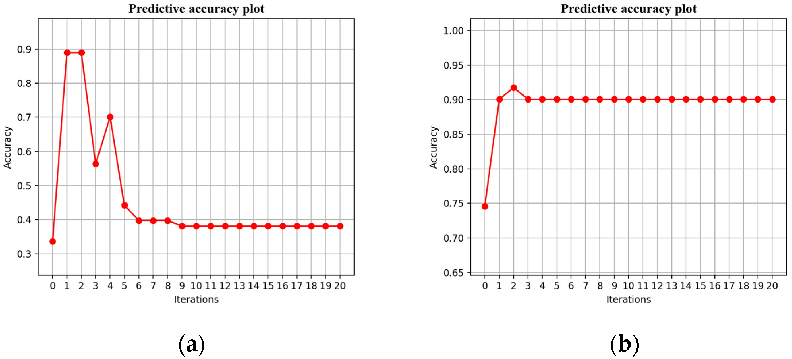
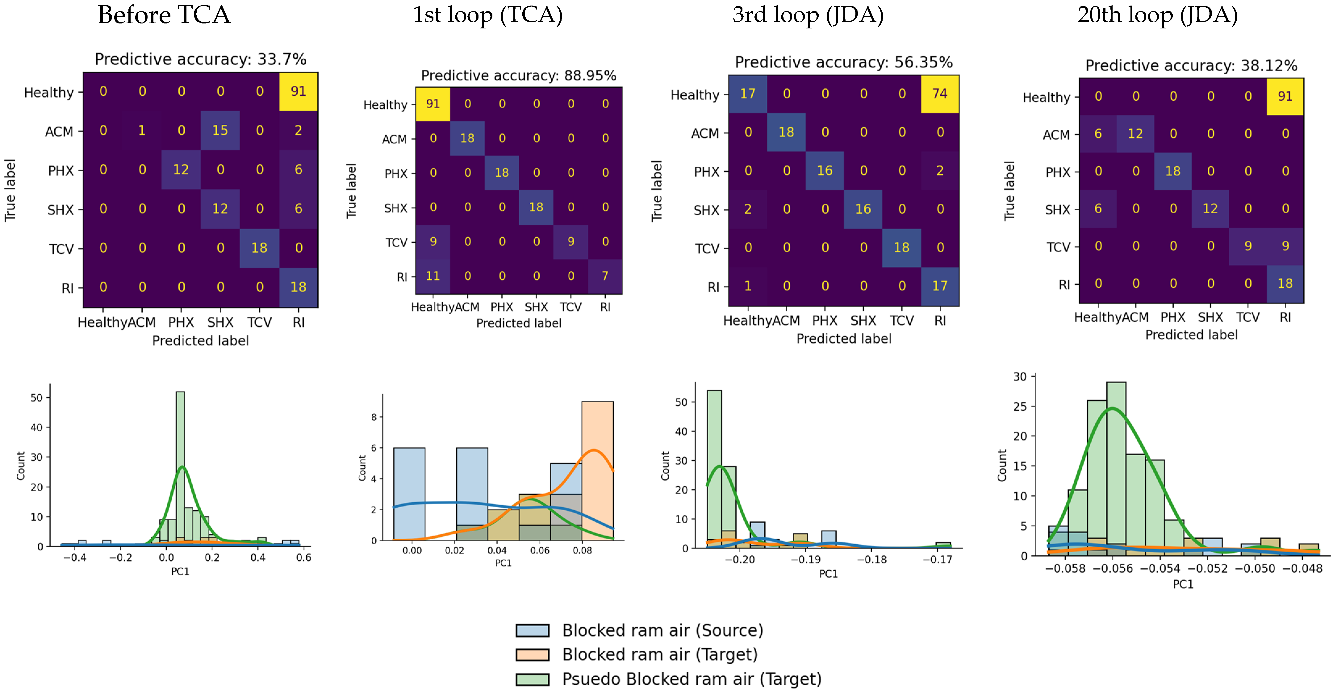
4.2. TL Approach: TCA and JDA

Aiming to reduce the effect of a domain shift, a TL approach for solving the fault diagnosis problem is developed based on TCA and JDA, using k-NN as the classifier. Two important parameters to be determined for the TCA and JDA algorithms are the value of λ, which controls the level of optimisation and the dimensions of the features.
The value of λ is to be determined first while holding the feature dimension at 6. The predictive accuracy for the target domain cases varies with the value of λ, as plotted in Figure 9. For TCA, the predictive accuracy shows a general increasing trend as λ decreases from 0.1 to 0.001 and remains constant at 97.99% for λ ≤ 0.0007. For JDA, the predictive accuracy stays around 40% for λ between 0.1 and 0.003 and jumps to around 95% for λ smaller than 0.0002. Hence, the optimal value of λ for both TCA and JDA was taken as 0.0001.
Holding λ at 0.0001, the dimensions of features have to be determined. Figure 10 plots the target domain predictive accuracy against the dimension of the features. For both TCA and JDA, the predictive accuracy rises considerably when the dimension of features increases from one to four and remains roughly constant when using six or more dimensions. Therefore, six was determined to be the optimal dimension for the transformed features in TCA and JDA.
Using λ = 0.0001 and holding the transformed feature dimension at six, the TL-based diagnostic algorithm with TCA and JDA significantly improved the target domain prediction accuracy. Compared with the 41.99% predictive accuracy of the non-TL approach, the TL approach increased the target domain predictive accuracy to 97.97% by TCA and 92.82% by JDA. The confusion matrices for both cases are plotted in Figure 11.
To justify the significant improvement made by the TL-based approach, it is expected that TCA and JDA align the distribution discrepancy between the source and target domains. Two observations support this claim.
The first piece of evidence is provided by calculating the MMD distance between the source and target domain features. Before and after applying TCA and JDA to the data, the MMD distance between the source domain features and target domain features was calculated to be 4.9 × 10⁻². This distance was reduced to 6.2 × 10⁻⁷ by TCA and to 4.6 × 10⁻⁵ by JDA, which means that both TCA and JDA significantly reduced the distribution discrepancy.
The second confirmation was achieved through visualisation. To visualise the six-dimensional data in two-dimensional plots, t-distributed stochastic neighbour embedding (t-SNE) is employed as the dimensionality reduction technique, because it performs the non-linear mapping of high-dimensional data onto a low-dimensional space, and many relevant studies have reported the successful application of t-SNE to visualise engineering data [14,33,34]. Using t-SNE, the source and target domain cases are plotted in Figure 12. The source domain cases are marked with dots, and the target domain cases are marked with crosses. Different colours were used to differentiate cases under each health state. It should be mentioned that the labels in the target domain have only been used to plot the cases, and they are not known by the algorithm. In Figure 12, the elimination of the domain shift is achieved when the dots and crosses of the same colour coincide. While this has not been observed, what has been observed is that the dots and crosses of the same colour move much closer after TCA and JDA than without TL, as shown by the comparison between Figure 12a–c. It can also be observed in Figure 12b,c that most of the source domain cases and the target domain cases of the same true label are sufficiently close as to be viewed as one cluster. Hence, the classifier trained with source domain cases would have a much higher predictive accuracy for the transferred target domain cases, which results in the significant improvement by the TL approach compared to the non-TL approach.

5. Expanding the Transfer Scenarios of the TL-Based Diagnostic Algorithm

After demonstrating that the TL approach by TCA and JDA performed well in the transfer scenario from 28k ft to 41k ft, further tests were performed using the other two operating conditions. This is to test the ability of this TL-based solution to generalise under wider transfer scenarios. The wider transfer scenarios in this section will also allow a more meaningful comparison between the TCA and JDA algorithms. The transfer scenarios were expanded in two ways. In Section 5.1, the transfer scenarios are expanded to include all four altitudes where the ECS simulation data are obtained. The cruise condition at 35,000 ft and the ground-running condition are two scenarios that have not been exposed to the algorithm when it was tuned in the last section. In Section 5.2, the target domain cases will have different compositions than the source domain, which simulates real-life scenarios where data collected could contain an arbitrary proportion of cases under each health state.

5.1. Transfer between Four Operating Conditions

The target domain predictive accuracies across the twelve possible transfer scenarios, based on the four operating conditions, are shown in Table 4; each row contains a target domain condition, and each column contains a source domain condition. In Table 4, the highest result(s) under each scenario have also been highlighted. With a minimum predictive accuracy of 88.95% and an average predictive accuracy of 94.89%, it can be concluded that TCA is accurate and reliable in the expanded range of operating conditions and demonstrates good generalisability.
JDA has improved the accuracy from the first TCA loop in one of the transfer scenarios, from Ground to 35k ft, where JDA increased the predictive accuracy to 92.82% compared to 92.27% by the TCA loop. This improvement demonstrates the benefit of the predictive accuracy obtained by aligning conditional distributions. However, in general, JDA performs worse than TCA in these expanded transfer scenarios, achieving a lower average predictive accuracy of 78.87% and an accuracy of less than 50% for three of the transfer scenarios. As a result, the diagnostic algorithm based on JDA does not have good generalisability in these cases.
The lack of generalisability for JDA on this dataset can be explained in terms of the characteristics of the JDA algorithm. Because the calculation of the target domain conditional distributions is based on pseudo labels rather than true labels, any wrongly predicted pseudo labels will result in a calculation of a conditional distribution that deviates from the true conditional distribution. This design allows JDA to work for target domains with no labels, yet an inevitable flaw would appear when too many pseudo labels are incorrectly predicted in any one of the JDA iterations.
Figure 13 and Figure 14 are used to explain such behaviour with one example scenario, where JDA produces a low accuracy at convergence, which is the transfer from 28k ft to Ground conditions. Figure 13a,b plots the predictive accuracy at each iteration, with the 0th iteration noting the predictive accuracy without TCA or JDA, the 1st iteration being the TCA loop, and the 2nd to 20th iterations being the JDA loops. Figure 13a is plotted for the scenario of interest, and to compare with a transfer scenario were JDA produces a high predictive accuracy at convergence, Figure 13b is plotted for the transfer from 35k ft to 28k ft. It was observed that the accuracy fluctuated only moderately during the JDA iterations. Moreover, most scenarios where JDA achieves high accuracy follow a similar trend, as shown in Figure 13b. Hence, a sharp reduction, such as that found at the 3rd iteration in Figure 13a, is identified as a unique feature for cases with low JDA accuracy. How it results in low accuracy is described as follows. The sharp reduction in the 3rd iteration in Figure 13a represents the prediction of many incorrect pseudo labels. The incorrect pseudo labels would have a cascading effect on the consecutive JDA loops and is hard for the accuracy to recover, because the conditional distribution calculated in the next loop is based on the large quantity of incorrect pseudo labels that will make it deviate further from the true conditional distribution. Then, in the next loop, the alignment of the source and target domain distribution will be misled by the incorrectly predicted conditional distribution, which potentially leads to more wrongly predicted pseudo labels at the end of the loop. Therefore, the predictive accuracy of JDA at convergence could be considerably lower than that of the TCA loop.
Figure 14 shows the process of increasing incorrect pseudo labels for this transfer scenario from 28k ft to Ground as a result of the process described above. From the confusion matrix on Figure 14 (top), the reduction in accuracy after the TCA loop is due to more and more cases being misclassified as RI blockage. To illustrate the distribution of these misclassified RI blockage cases, the distribution of the first principal component value is plotted on Figure 14 (bottom) as a representation of the conditional distribution of cases with pseudo label or true label of RI blockage. Source domain cases with real RI blockage labels are shown by the blue distribution. Target domain cases with real RI blockage labels are shown by the orange distribution, and target domain cases with pseudo RI blockage labels are shown by the green distribution. Thus, an accurate prediction of all target domain RI blockage cases would be when the orange and green distributions coincide. However, this was not observed and instead, from the 3rd iteration, cases in the green distribution exceeds those in orange distribution, because there were healthy cases mistaken as RI blockage cases. Then, applying JDA to the healthy cases misclassified into RI blockage cases would continue to cause deterioration until the final loop. By the 20th loop, all healthy cases were misclassified.

5.2. Transfer with Different Case Compositions in the Target Domain

Previous experiments have been carried out with the same case composition in the source and target domain, which consists of 91 healthy cases and 18 cases for each degradation labels including PHX fault, SHX fault, ACM fault, TCV fault, and RI blockage. However, it is unreasonable to expect the same composition of cases when collecting real-life data. Hence, there is a need to test TL-based diagnostic algorithms with different case compositions in the target domain.
Five different compositions of the cases in the target domain were simulated, and the details are listed in Table 5. In composition 1, half of all healthy cases are removed, which makes the proportion of faulty cases higher in the target domain than in the source domain. This may not be realistic, because normally an ECS generates abundant healthy cases compared to faulty cases, but it is worth examining if the opposite scenario affects the algorithm. In composition 2, the RI blockage cases with minor and severe degradation levels are removed to leave only one degradation level for RI blockage cases in the target domain, which corresponds to a real-life scenario where faults collected are not in multiple degradation levels. The same operation is done to both RI blockage cases and PHX fault cases in composition 3. In composition 4, all RI blockage cases are removed from the target domain, and in composition 5, all RI blockage cases and TCV fault cases are removed from the target domain. Compositions 4 and 5 simulate scenarios in which data for certain fault modes have not been collected.
This increases the distribution discrepancy between the source and target domains, and hence, it tests how the TCA- and JDA-based algorithms handle larger distribution discrepancy.
Table 6 shows the predictive accuracies of TCA and JDA. The number in the bracket after each target domain operating condition corresponds to the case composition number introduced in Table 5. Each row in Table 6 contains the predictive accuracy of TCA and JDA in a particular target domain after transferring knowledge from different source domain conditions. Comparing TCA and JDA, the highest result(s) under each scenario have been highlighted.
It was found that JDA achieves a higher predictive accuracy than TCA in several transfer scenarios. This improvement in accuracy highlights the advantage of aligning the conditional distribution in addition to aligning the marginal distribution by TCA. However, in general, JDA does not perform as well as TCA, generating an average accuracy of 77.47% compared to 95.22% from TCA. This is partly because by making the target domain case composition different from the source domain, it is more likely to have many incorrectly predicted pseudo labels in one of the JDA iterations. Because of the reason described in Section 5.1, this would eventually lead to a low predictive accuracy for JDA at convergence. Comparing the five compositions in the target domain, compositions 2–5 have larger distribution discrepancy between the source and target domain cases than composition 1, which could make JDA perform worse. For example, the transfer from 28k ft to Ground shows very low JDA predictive accuracy particularly in composition 2–5.
In addition, although JDA is usually considered being able to generate more accurate prediction that TCA [21], same trend does not generally hold for the ECS dataset tested in this paper, as shown in both Table 4 and Table 6. A unique feature about this dataset which could explain is that there may only be minor differences between some cases with different labels (e.g., minor PHX fault cases with healthy cases), as shown in Figure 2. This makes the iterative conditional alignment in JDA particularly vulnerable to misclassification. As a result, JDA is considered a less accurate method with less ability to generalise in this dataset.
Regarding TCA, it has achieved a high average predictive accuracy of 95.22%, with a minimum accuracy of 69.43% across all transfer scenarios, as shown in Table 6. It can be concluded that TCA has demonstrated its ability to generalise when the target domain data are simultaneously under a new operating condition and consist of a different and incomplete composition of cases than the source domain.

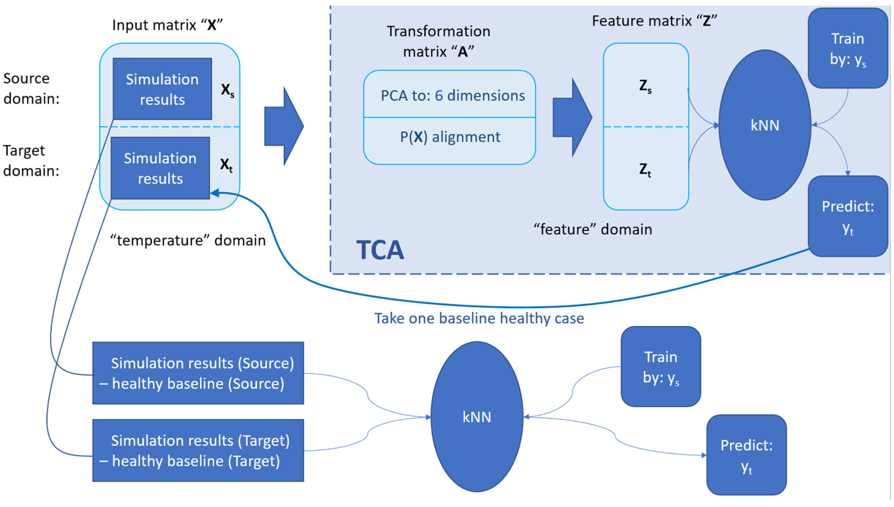
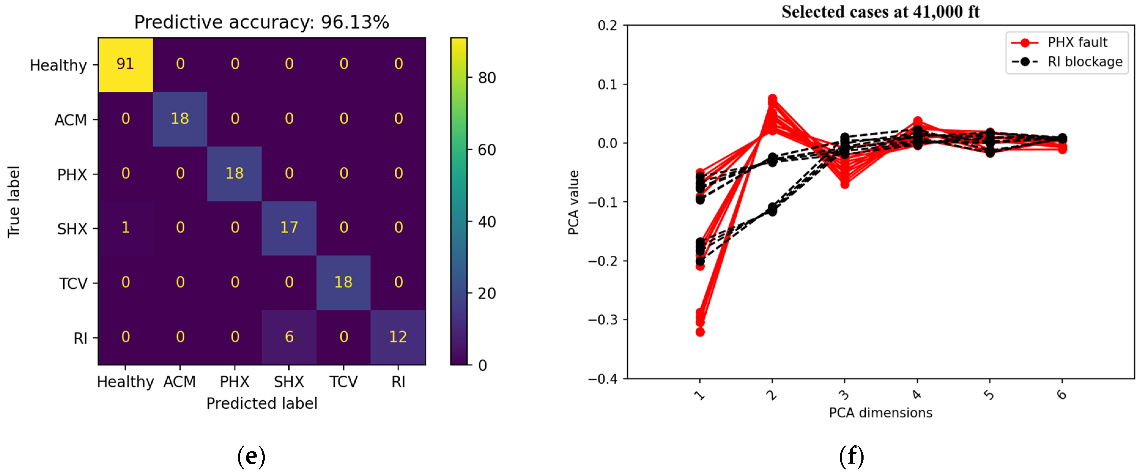
6. An Alternative TL-Based Fault Diagnosis Process for Unlabelled Target Domain Using TCA

Following a close inspection of all the confusion matrices of the TCA results in Section 5, one major finding is that the prediction of the healthy cases is particularly accurate for all transfer scenarios. Table 7 demonstrates this point by the predictive accuracy and precision for target domain healthy cases, where the predictive accuracy is calculated by the true positive rate (TPR) for healthy cases, and the precision is calculated by the positive predictive rate (PPV) for the healthy cases. PPV is of interest, since it calculates the proportion of true healthy cases among all healthy cases predicted.
From Table 7, both predictive accuracy and precision are high for TCA after averaging over all transfer scenarios, at 98.30% and 94.56%, respectively. Furthermore, the minimum precision, 69.70%, stands above 50%, which means the correct healthy cases can be found in larger proportion than the incorrect healthy cases in the worst performing scenario. In 95% of all transfer scenarios tested, the precision is found to be above 80%, which indicates the true healthy case dominates in all the predicted healthy cases. Consequently, it is safe to conclude that TCA predicts healthy labels accurately and reliably across all transfer scenarios on Table 7.
This feature of TCA is of particular interest because, with the identification of the healthy label in the target domain, an alternative solution for the fault diagnosis for the unlabelled target domain can now be designed and tested if it can deliver better results than TCA. It is a common practice to use deviation from the healthy baseline as the basis for fault diagnosis in engineering scenarios. While this was not possible by the assumption of only unlabelled data in target domain, the accurate prediction of healthy labels enables this approach for the problem of interest. Existing works in ECS fault diagnosis also adopt deviation data from a healthy baseline, such as the work by Skliros et al. [35] and the work of Liu et al. [36], who used the deviation between the measured signal and baseline data to diagnose ECS faults effectively in multiple flight phases, the identification of the healthy label in the target domain enables the establishment of baseline data, so that deviation from the baseline can be used instead of nominal data in order to allow better fault identification.
The architecture of the alternative solution is shown in Figure 15. First, TCA was performed as normal, and at the end of the TCA loop, a healthy case could be identified from the target domain. In contrast to the TCA approach, the other labels predicted by TCA are not considered as the final label prediction. At the end of the first step, the target domain no longer has only unlabelled data because it has one healthy case labelled. In the second step, a healthy case is chosen as the baseline case in the source domain, and the case labelled healthy from step 1 serves as the target domain counterpart. All cases in the source domain and the target domain are then subtracted from the respective baseline healthy case in each domain. This step should help to reduce the domain shift between the source and target domain, since all cases now bear the deviation data from the healthy baseline case. The cases with deviation data in the source and target domains should share a similar pattern when they are in the same health state, which would make a classifier trained in the source domain accurate when directly applied to the target domain. For instance, it is clear from Figure 2 that a PHX fault can be identified by rising temperature at PHX outlet and SHX inlet than the healthy case, and this trend is invariant across the operating conditions. In the last step, the k-NN trained by the source domain deviation data is applied directly to the target domain deviation data for label prediction.
By applying this alternative solution to the transfer between the four operating conditions, the predictive accuracy was recorded, as shown in Table 8. The predictive accuracy following the non-TL approach (kNN) and TCA are also recorded in Table 8 for comparison. The non-TL approach (kNN) has adopted PCA instead of mRMR as the dimensionality reduction technique to align with TCA.
Compared with the non-TL approach, the alternative method using deviation data produces higher predictive accuracy in most of the scenarios tested, and the average accuracy shows an improvement from 63.72% to 72.70%. Because k-NN is applied for label prediction in a similar way for the two methods, with the only difference being whether deviation data from a healthy baseline are used, this improvement in accuracy justifies how the designed alternative method effectively reduces the domain shift, alleviating the problem illustrated in Figure 8. Compared with TCA, the alternative method also achieved higher accuracy in one transfer scenario. This proves that taking the deviation data from a healthy baseline case is indeed a useful way to reduce the influence of the domain shift and improve the predictive accuracy for ECS data under different operating conditions.
In general, the alternative method did not perform better than TCA, as shown in Table 8. TCA still produced higher predictive accuracy in most transfer scenarios, and the average accuracy of 94.89% also outperforms the 72.70% accuracy by the alternative method. The reason for this is that, although taking the deviation data from a healthy baseline case reduces the influence of domain shift, it cannot effectively distinguish similar cases under different classes. For example, in the transfer scenario from Ground to 41k ft, despite the alternative method of feeding deviation data instead of nominal data to the k-NN classifier improving the diagnostic accuracy from 54.14% to 61.88%, TCA produced a much higher accuracy of 96.13%. Closer examination into the misclassification details revealed that both non-TL method and the alternative method show confusion between PHX fault and RI Blockage cases, whereas such confusion is not found for TCA, as shown in Figure 16a,c,e.
To investigate how TCA distinguishes confused cases, while other methods do not, the cases for the confused classes in the target domain are plotted in Figure 16. Figure 16b,d show the difference between the nominal data and the deviation data. Because the original temperature profile shows overlapping between the two classes in Figure 16a, taking deviation from a common baseline case cannot resolve the overlapping, as shown in Figure 16d. However, the situation is different after applying TCA. As Figure 16f shows, the two confused classes can be distinguished with the application of TCA. Therefore, TCA has demonstrated its ability to distinguish confused classes in the unlabelled target domain based on labelled source domain data, which gives it better diagnostic accuracy than feeding the k-NN classifier with deviation data.

7. Conclusions and Limitations

This study on the application of TL to cross-condition fault diagnosis of an aircraft ECS has demonstrated that TL-based algorithms, TCA and JDA, significantly improve the diagnosis accuracy of unlabelled ECS data under unknown operating conditions, compared to the non-TL approach. While the non-TL approach produces 63.72% average predictive accuracy across the four operating conditions, TCA improves the accuracy to 94.89%, and JDA achieves an average accuracy of 78.87%. Testing TCA and JDA on target domain data with different composition of cases than the source domain, TCA achieved average accuracy of 95.22%, and JDA has 77.47% accuracy over all scenarios. Contrary to the common belief that JDA achieves higher accuracy over TCA, the results above show that, for the dataset used, TCA is a more robust and accurate TL algorithm than JDA. This is because the accuracy of JDA is vulnerable to false pseudo label prediction during its iterative process, and the similarity of cases with different labels is likely to lead to such cases.
Although unlabelled target domains are assumed, the accurate prediction of healthy cases from TCA enabled the conversion of nominal data to deviation data from healthy baselines, which is a common practice in fault diagnosis studies. Using deviation data, the predictive accuracy following the non-TL approach has improved to 72.70%, proving its value for cross-condition fault diagnosis problems. However, TCA remains the best strategy for this problem, owing to its ability to distinguish between overlapping classes using source domain knowledge.
Regarding the real-life application of fault diagnosis on ECS, certain limitations of this study are worth considering. Firstly, imperfection in real ECS data may exceed the range considered in this study. For example, incorrect data collection in case of sensor malfunction would produce outliers in the dataset. How these outliers affect the TL-based fault diagnosis has not been discussed. Secondly, this paper has focused on single fault modes, but multiple faults are possible at the same time in real operations of ECS. Hence, advanced methods need to be developed to cover the possibility of multiple fault modes.

Author Contributions

Conceptualization, L.J., C.M.E. and I.K.J.; formal analysis, L.J., C.M.E. and I.K.J.; investigation, L.J.; writing—original draft preparation, L.J.; writing—review and editing, L.J., C.M.E. and I.K.J. All authors have read and agreed to the published version of the manuscript.

Funding

This research received no external funding.

Institutional Review Board Statement

Not applicable.

Data Availability Statement

The data presented in this study are available on request from the corresponding author. The data are not publicly available due to copyright of the simulation software used to generate them.

Conflicts of Interest

The authors declare no conflict of interest.

Abbreviations

The following abbreviations are used in this manuscript:
ACMAir cycle machine
CNNConvolutional neural network
ECSEnvironmental control system
JDAJoint distribution alignment
k-NNk-nearest neighbour
MLMachine learning
MMDMaximum mean discrepancy
PACKPassenger Air Conditioner
PCAPrincipal component analysis
PHXPrimary heat exchanger
RIRam air inlet
SESACSimscape Environmental Control System Simulation under All Conditions
SHXSecondary heat exchanger
TCATransfer component analysis
TCVTemperature control valve
TLTransfer learning
t-SNEt-distributed stochastic neighbour embedding

References

  1. Pinto, R.; Gonçalves, G. Application of Artificial Immune Systems in Advanced Manufacturing. Array 2022, 15, 100238. [Google Scholar] [CrossRef]
  2. Tu, W.; Fang, J.; He, Y.; Huang, J. Application Analysis of Machine Learning in Fault Diagnosis: A Bibliometric Analysis. J. Phys. Conf. Ser. 2020, 1629, 012020. [Google Scholar] [CrossRef]
  3. Van Tung, T.; Yang, B.-S. Machine Fault Diagnosis and Prognosis: The State of The Art. Int. J. Fluid Mach. Syst. 2009, 2, 61–71. [Google Scholar] [CrossRef]
  4. Li, W.; Huang, R.; Li, J.; Liao, Y.; Chen, Z.; He, G.; Yan, R.; Gryllias, K. A Perspective Survey on Deep Transfer Learning for Fault Diagnosis in Industrial Scenarios: Theories, Applications and Challenges. Mech. Syst. Signal Process 2022, 167, 108487. [Google Scholar] [CrossRef]
  5. Vachtsevanos, G.; Lewis, F.; Roemer, M.; Hess, A.; Wu, B. Intelligent Fault Diagnosis and Prognosis for Engineering Systems; Wiley: Hoboken, NJ, USA, 2007; pp. 1–434. [Google Scholar] [CrossRef]
  6. Qian, W.; Li, S.; Yi, P.; Zhang, K. A Novel Transfer Learning Method for Robust Fault Diagnosis of Rotating Machines under Variable Working Conditions. Measurement 2019, 138, 514–525. [Google Scholar] [CrossRef]
  7. Chen, C.; Shen, F.; Xu, J.; Yan, R. Domain Adaptation-Based Transfer Learning for Gear Fault Diagnosis under Varying Working Conditions. IEEE Trans. Instrum. Meas. 2021, 70. [Google Scholar] [CrossRef]
  8. An, Y.; Zhang, K.; Liu, Q.; Chai, Y.; Huang, X. Deep Transfer Learning Network for Fault Diagnosis under Variable Working Conditions. In Proceedings of the 2021 CAA Symposium on Fault Detection, Supervision, and Safety for Technical Processes (SAFEPROCESS), Chengdu, China, 17–18 December 2021. [Google Scholar] [CrossRef]
  9. Zhu, J.; Chen, N.; Shen, C. A New Deep Transfer Learning Method for Bearing Fault Diagnosis under Different Working Conditions. IEEE Sens. J. 2020, 20, 8394–8402. [Google Scholar] [CrossRef]
  10. Yang, Q.; Zhang, Y.; Dai, W.; Pan, S.J. Transfer Learning; Cambridge University Press: Cambridge, UK, 2020; ISBN 9781139061773. [Google Scholar]
  11. Zheng, H.; Wang, R.; Yang, Y.; Yin, J.; Li, Y.; Li, Y.; Xu, M. Cross-Domain Fault Diagnosis Using Knowledge Transfer Strategy: A Review. IEEE Access 2019, 7, 129260–129290. [Google Scholar] [CrossRef]
  12. He, J.; Li, X.; Chen, Y.; Chen, D.; Guo, J.; Zhou, Y. Deep Transfer Learning Method Based on 1D-CNN for Bearing Fault Diagnosis. Shock. Vib. 2021, 2021, 6687331. [Google Scholar] [CrossRef]
  13. Xiao, D.; Huang, Y.; Zhao, L.; Qin, C.; Shi, H.; Liu, C. Domain Adaptive Motor Fault Diagnosis Using Deep Transfer Learning. IEEE Access 2019, 7, 80937–80949. [Google Scholar] [CrossRef]
  14. Li, B.; Zhao, Y.P.; Chen, Y. Bin Unilateral Alignment Transfer Neural Network for Fault Diagnosis of Aircraft Engine. Aerosp. Sci. Technol. 2021, 118, 107031. [Google Scholar] [CrossRef]
  15. Liu, S.; Wang, H.; Tang, J.; Zhang, X. Research on Fault Diagnosis of Gas Turbine Rotor Based on Adversarial Discriminative Domain Adaption Transfer Learning. Measurement 2022, 196, 111174. [Google Scholar] [CrossRef]
  16. Chowdhury, S.H.; Ali, F.; Jennions, I.K. A Review of Aircraft Environmental Control System Simulation and Diagnostics. Proc. Inst. Mech. Eng. G J. Aerosp. Eng. 2023, 237, 2453–2467. [Google Scholar] [CrossRef]
  17. Jennions, I.; Ali, F.; Miguez, M.E.; Escobar, I.C. Simulation of an Aircraft Environmental Control System. Appl. Therm. Eng. 2020, 172, 114925. [Google Scholar] [CrossRef]
  18. Jennions, I.; Ali, F. Assessment of Heat Exchanger Degradation in a Boeing 737-800 Environmental Control System. J. Therm. Sci. Eng. Appl. 2021, 13, 061015. [Google Scholar] [CrossRef]
  19. Lei, Y.; Yang, B.; Jiang, X.; Jia, F.; Li, N.; Nandi, A.K. Applications of Machine Learning to Machine Fault Diagnosis: A Review and Roadmap. Mech. Syst. Signal Process 2020, 138, 106587. [Google Scholar] [CrossRef]
  20. Yang, B.; Lei, Y.; Jia, F.; Xing, S. An Intelligent Fault Diagnosis Approach Based on Transfer Learning from Laboratory Bearings to Locomotive Bearings. Mech. Syst. Signal Process 2019, 122, 692–706. [Google Scholar] [CrossRef]
  21. Long, M.; Wang, J.; Ding, G.; Sun, J.; Yu, P.S. Transfer Feature Learning with Joint Distribution Adaptation. In Proceedings of the IEEE International Conference on Computer Vision, Sydney, NSW, Australia, 1–8 December 2013. [Google Scholar] [CrossRef]
  22. Azari, M.S.; Flammini, F.; Santini, S.; Caporuscio, M. A Systematic Literature Review on Transfer Learning for Predictive Maintenance in Industry 4.0. IEEE Access 2023, 11, 12887–12910. [Google Scholar] [CrossRef]
  23. Xie, Y.; Liu, C.; Huang, L.; Duan, H. Ball Screw Fault Diagnosis Based on Wavelet Convolution Transfer Learning. Sensors 2022, 22, 6270. [Google Scholar] [CrossRef]
  24. Zhang, L.; Duan, L. Cross-Scenario Transfer Diagnosis of Reciprocating Compressor Based on CBAM and ResNet. J. Intell. Fuzzy Syst. 2022, 43, 5929–5943. [Google Scholar] [CrossRef]
  25. Li, M.; Sun, Z.-H.; He, W.; Qiu, S.; Liu, B. Rolling Bearing Fault Diagnosis under Variable Working Conditions Based on Joint Distribution Adaptation and SVM. In Proceedings of the International Joint Conference on Neural Networks (IJCNN), Glasgow, UK, 19–24 July 2020. [Google Scholar] [CrossRef]
  26. Xu, W.; Wan, Y.; Zuo, T.Y.; Sha, X.M. Transfer Learning Based Data Feature Transfer for Fault Diagnosis. IEEE Access 2020, 8, 76120–76129. [Google Scholar] [CrossRef]
  27. Tang, Y.; Dou, L.; Zhang, R.; Zhang, X.; Liu, W. Deep Transfer Learning-Based Fault Diagnosis of Spacecraft Attitude System. In Proceedings of the 39th Chinese Control Conference (CCC), Shenyang, China, 27–29 July 2020; pp. 4072–4077. [Google Scholar] [CrossRef]
  28. Guo, W.; Li, S.; Miao, Q.; Shandong-Keji-Daxue Tai’an, S. Institute of Electrical and Electronics Engineers A Cross Domain Feature Extraction Method for Bearing Fault Diagnosis Based on Balanced Distribution Adaptation. In Proceedings of the Prognostics and System Health Management Conference (PHM-Qingdao), Qingdao, China, 25–27 October 2019. [Google Scholar] [CrossRef]
  29. Pan, S.J.; Tsang, I.W.; Kwok, J.T.; Yang, Q. Domain Adaptation via Transfer Component Analysis. IEEE Trans. Neural Netw. 2011, 22, 199–210. [Google Scholar] [CrossRef]
  30. Wang, J. Everything about Transfer Learning and Domain Adapation. Available online: http://transferlearning.xyz (accessed on 4 September 2023).
  31. Peng, H.; Long, F.; Ding, C. Feature Selection Based on Mutual Information: Criteria of Max-Dependency, Max-Relevance, and Min-Redundancy. IEEE Trans. Pattern Anal. Mach. Intell. 2005, 27, 1226–1238. [Google Scholar] [CrossRef]
  32. Pedregosa, F.; Michel, V.; Grisel, O.; Blondel, M.; Prettenhofer, P.; Weiss, R.; Vanderplas, J.; Cournapeau, D.; Varoquaux, G.; Gramfort, A.; et al. Scikit-Learn: Machine Learning in Python. J. Mach. Learn. Res. 2011, 12, 2825–2830. [Google Scholar]
  33. Zhu, P.; Dong, S.; Pan, X.; Hu, X.; Zhu, S. A Simulation-Data-Driven Subdomain Adaptation Adversarial Transfer Learning Network for Rolling Element Bearing Fault Diagnosis. Meas. Sci. Technol. 2022, 33, 075101. [Google Scholar] [CrossRef]
  34. Ding, Y.; Jia, M.; Zhuang, J.; Cao, Y.; Zhao, X.; Lee, C.-G. Deep Imbalanced Domain Adaptation for Transfer Learning Fault Diagnosis of Bearings under Multiple Working Conditions. Reliab. Eng. Syst. Saf. 2023, 230, 108890. [Google Scholar] [CrossRef]
  35. Skliros, C.; Ali, F.; King, S.; Jennions, I. Aircraft System-Level Diagnosis with Emphasis on Maintenance Decisions. Proc. Inst. Mech. Eng. Part O J. Risk Reliab. 2022, 236, 1057–1077. [Google Scholar] [CrossRef]
  36. Liu, C.; Sun, J.; Wang, F.; Ning, S.; Xu, G. Bayesian Network Method for Fault Diagnosis of Civil Aircraft Environment Control System. Proc. Inst. Mech. Engineers. Part I J. Syst. Control Eng. 2020, 234, 662–674. [Google Scholar] [CrossRef]
Figure 1. Schematic of a Boeing 737–800 PACK with the air flow sequence labelled [16].
Applsci 13 13120 g001
Figure 2. (a) Temperature profile of PACK for operating condition A. (b) Temperature profile of PACK for operating condition B. (c) Temperature profile of PACK for operating condition C. (d) Temperature profile of PACK for operating condition D.
Applsci 13 13120 g002
Figure 3. An illustration of the general steps of feature-based transfer learning [20].
Applsci 13 13120 g003
Figure 4. Distribution of the first principal component value for cases at 28,000 ft and 41,000 ft, plotted to represent the discrepancy in marginal distribution.
Applsci 13 13120 g004
Figure 5. Distribution of the first principal component value for cases of the same label at 28,000 ft and 41,000 ft, plotted to represent the discrepancy in conditional distribution.
Applsci 13 13120 g005aApplsci 13 13120 g005b
Figure 6. k-NN predictive accuracy against input dimension.
Applsci 13 13120 g006
Figure 7. Confusion matrix plot for target domain data following the non-TL approach.
Applsci 13 13120 g007
Figure 8. An example of misclassification following the non-TL approach.
Applsci 13 13120 g008
Figure 9. Predictive accuracy of TCA and JDA against value of λ, using 6 features.
Applsci 13 13120 g009
Figure 10. Predictive accuracy of TCA and JDA against dimension of transformed features, when λ = 0.0001.
Applsci 13 13120 g010
Figure 11. Confusion matrix plot of results by: (a) TCA, (b) JDA.
Applsci 13 13120 g011
Figure 12. (a) 2D t-SNE visualisation of cases from source and target domain without TL. (b) 2D t-SNE visualisation of cases from source and target domain after TCA. (c) 2D t-SNE visualisation of cases from source and target domain after JDA.
Applsci 13 13120 g012
Figure 13. Predictive accuracy at each iteration in the transfer scenario: (a) from 28,000 ft to Ground, (b) from 35,000 ft to 28,000 ft.
Applsci 13 13120 g013
Figure 14. Confusion matrix plot (top) and plot of distribution of cases with RI blockage label (bottom) for the transfer from 28,000 ft to Ground conditions at each key iteration.
Applsci 13 13120 g014
Figure 15. The architecture of an alternative solution enabled by TCA.
Applsci 13 13120 g015
Figure 16. (a) Confusion matrix for non-TL approach using nominal data (Ground–41k ft). (b) Plot of cases as nominal data for the confused classes in the target domain. (c) Confusion matrix for non-TL approach using deviation data (Ground—41k ft). (d) Plot of cases as deviation data for the confused classes in the target domain. (e) Confusion matrix for TCA results (Ground—41k ft). (f) Plot of cases after applying TCA for the confused classes in the target domain.
Applsci 13 13120 g016aApplsci 13 13120 g016b
Table 1. Summary of all degradation levels simulated for each failure mode considered in the PACK simulation.
Fault ModeDegradation Degree
MinorMediumSevere
ACM fault25%50%75%
PHX fault20%50%80%
SHX fault20%50%80%
RI blockage 25%50%75%
Degraded state
TCV fault (normally 15°–18°)Undershoot:
Fixed at 10°
Overshoot:
Fixed at 23°
Table 2. Summary of the key parameters for the four operating conditions simulated.
Operating ConditionAltitude (ft)Bleed Temperature (K)Bleed Pressure (kPa)Ram Air Temperature (K)Mean Target Temperature (K)Mean Target Mass Flow Rate ( k g · s 1 ) Number of Cases
A0461.2320297.0266.50.6091 healthy-state cases;
90 faulty-state cases
B28,000469.0193232.7291.20.4591 healthy-state cases;
90 faulty-state cases
C35,000470.7234245.5284.90.4391 healthy-state cases;
90 faulty-state cases
D41,000469.3190216.7298.10.4291 healthy-state cases;
90 faulty-state cases
Table 3. Summary of operating condition in source and target domain for developing TL-based diagnosis algorithm.
DomainAltitude (ft)Bleed Temperature (K)Bleed Pressure (kPa)Ram Air Temperature (K)Target Temperature (K)Target Mass Flow Rate ( k g · s 1 ) Number of Cases
Source28,000469.0193232.7291.2 ± 100.45 ± 0.0291 healthy-state cases;
90 faulty-state cases
Target41,000469.3190216.7298.1 ± 100.42 ± 1091 healthy-state cases;
90 faulty-state cases
Table 4. Predictive accuracy of TCA and JDA for the transfer across four operating conditions.
TCA:
Prediction Accuracy (%)
JDA:
Prediction Accuracy (%)
SOURCESOURCE
Ground28,000 ft35,000 ft41,000 ftGround28,000 ft35,000 ft41,000 ft
TARGETGround-88.9590.0690.06-38.1241.9990.06
28,000 ft100.00-94.4895.5893.37-91.7164.64
35,000 ft92.2793.37-100.0092.8247.51-100.00
41,000 ft96.1397.79100.00-93.3792.82100.00-
Average: 94.89Average: 78.87
Table 5. Different case composition the target domain.
Cases Composition NumberScenario Simulated in Target DomainComposition of Cases in Source Domain (S) and Target Domain (T)
1A fault-rich ECSS: 91 H, 18 ACM, 18 PHX, 18 SHX, 18 TCV, 18 RI
T: 46 H, 18 ACM, 18 PHX, 18 SHX, 18 TCV, 18 RI
2Less degradation level in 1 fault modeS: 91 H, 18 ACM, 18 PHX, 18 SHX, 18 TCV, 18 RI
T: 91 H, 18 ACM, 18 PHX, 18 SHX, 18 TCV, 6 RI (mediums only)
3Less degradation level in 2 fault mode 2S: 91 H, 18 ACM, 18 PHX, 18 SHX, 18 TCV, 18 RI
T: 91 H, 18 ACM, 6 PHX (mediums only), 18 SHX, 18 TCV, 6 RI (mediums only)
4No data for 1 fault modeS: 91 H, 18 ACM, 18 PHX, 18 SHX, 18 TCV, 18 RI
T: 91 H, 18 ACM, 18 PHX, 18 SHX, 18 TCV, 0 RI
5No data for 2 fault modesS: 91 H, 18 ACM, 18 PHX, 18 SHX, 18 TCV, 18 RI
T: 91 H, 18 ACM, 18 PHX, 18 SHX, 0 TCV, 0 RI
Table 6. Predictive accuracy by TCA and JDA with different case composition in the target domain.
TCA:
Prediction Accuracy (%)
JDA:
Prediction Accuracy (%)
SOURCESOURCE
Ground28,000 ft35,000 ft41,000 ftGround28,000 ft35,000 ft41,000 ft
TARGETGround (1)-85.2986.7688.97-55.1554.4190.44
Ground (2)-91.1292.9092.90-36.0990.5395.27
Ground (3)-69.4392.3691.08-30.5794.2734.39
Ground (4)-93.2596.3296.32-31.2992.6498.77
Ground (5)-100.0095.8695.86-26.2128.2828.97
28,000 ft (1)100.00-91.1895.5991.18-87.5091.91
28,000 ft (2)100.00-97.6398.8298.82-44.3844.97
28,000 ft (3)98.09-98.7395.5498.09-42.0442.04
28,000 ft (4)100.00-97.5597.5569.94-97.5597.55
28,000 ft (5)100.00-91.0399.31100.00-96.5597.24
35,000 ft (1)88.9783.82-100.0088.2490.44-100.00
35,000 ft (2)93.4997.63-100.0094.6792.90-98.82
35,000 ft (3)88.5493.63-96.1892.9994.90-98.73
35,000 ft (4)94.4896.32-97.5595.0948.47-100.00
35,000 ft (5)96.5595.17-97.9360.0027.59-95.17
41,000 ft (1)93.3891.9199.26-92.6590.44100.00-
41,000 ft (2)100.0097.04100.00-98.8295.27100.00-
41,000 ft (3)94.2796.1898.73-98.7396.18100.00-
41,000 ft (4)98.7798.1698.77-80.3725.77100.00-
41,000 ft (5)100.0097.9399.31-82.0723.4599.31-
Average: 95.22Average: 77.47
Table 7. The predictive accuracy and precision of healthy cases in the target domain by TCA.
TCA:
TPR on Healthy Cases (%)
TCA:
PPV on Healthy Cases (%)
SOURCESOURCE
Ground28,000 ft35,000 ft41,000 ftGround28,000 ft35,000 ft41,000 ft
TARGETGround (1)-100.00100.00100.00-69.7071.8875.41
Ground (2)-100.00100.00100.00-85.8588.3588.35
Ground (3)-65.93100.00100.00-80.0088.3591.00
Ground (4)-100.00100.00100.00-89.2293.8193.81
Ground (5)-100.00100.00100.00-100.0095.7993.81
28,000 ft (1)100.00-100.00100.00100.00-85.1988.46
28,000 ft (2)100.00-100.00100.00100.00-100.0097.85
28,000 ft (3)96.70-100.00100.00100.00-98.9196.81
28,000 ft (4)100.00-100.00100.00100.00-100.0097.85
28,000 ft (5)100.00-90.11100.00100.00-100.00100.00
35,000 ft (1)100.0086.96-100.0093.8881.63-100.00
35,000 ft (2)96.70100.00-100.0097.7895.79-100.00
35,000 ft (3)87.9195.60-100.0097.5694.57-95.79
35,000 ft (4)92.31100.00-100.0097.6795.79-96.81
35,000 ft (5)96.70100.00-100.0098.8893.81-97.85
41,000 ft (1)100.00100.00100.00-95.8386.7997.87-
41,000 ft (2)100.00100.00100.00-100.0096.81100.00-
41,000 ft (3)90.11100.00100.00-100.0094.7997.85-
41,000 ft (4)98.90100.00100.00-100.0097.85100.00-
41,000 ft (5)100.00100.00100.00-100.0097.85100.00-
Average: 98.30Average: 94.56
Table 8. Target domain predictive accuracy by different approaches to the problem.
Fault Diagnostic MethodTransfer ScenarioAverage
Ground—28,000 ftGround—35,000 ftGround—41,000 ft28,000 ft—Ground28,000 ft–35,000 ft28,000 ft–41,000 ft35,000 ft–Ground35,000 ft–28,000 ft35,000 ft–41,000 ft41,000 ft—Ground41,000 ft–28,000 ft41,000 ft–35,000 ft
kNN60.7733.1554.1425.9760.7796.6944.2074.0389.5047.5195.5882.3263.72
A healthy baseline case from TCA + kNN on deviation data67.4063.5461.8863.5460.7792.2770.1771.8282.8761.3396.1380.6672.70
TCA10092.2796.1388.9593.3797.7990.0694.4810090.0695.5810094.89
Disclaimer/Publisher’s Note: The statements, opinions and data contained in all publications are solely those of the individual author(s) and contributor(s) and not of MDPI and/or the editor(s). MDPI and/or the editor(s) disclaim responsibility for any injury to people or property resulting from any ideas, methods, instructions or products referred to in the content.

