Using the Weibull Accelerated Failure Time Regression Model to Predict Time to Health Events

Abstract

Clinical prediction models are commonly utilized in clinical practice to screen high-risk patients. This enables healthcare professionals to initiate interventions aimed at delaying or preventing adverse medical events. Nevertheless, the majority of these models focus on calculating probabilities or risk scores for medical events. This information can pose challenges for patients to comprehend, potentially causing delays in their treatment decision-making process. Our paper presents a statistical methodology and protocol for the utilization of a Weibull accelerated failure time (AFT) model in predicting the time until a health-related event occurs. While this prediction technique is widely employed in engineering reliability studies, it is rarely applied to medical predictions, particularly in the context of predicting survival time. Furthermore, we offer a practical demonstration of the implementation of this prediction method using a publicly available dataset.

1. Introduction

Clinical prediction models are commonly utilized in clinical practice to screen high-risk patients. This enables healthcare professionals to initiate interventions aimed at delaying or preventing adverse medical events. However, in the realm of the medical literature, most prediction models focus on estimating the probability of an event occurring or a condition developing over a specified time frame. For instance, there are well-known models like the Framingham 10-year risk of general cardiovascular disease [1] and FRAX, a tool for estimating 10-year fracture risk [2]. This information can pose challenges for patients to comprehend, potentially causing delays in their treatment decision-making process. In contrast, in engineering reliability research, it is commonplace to employ Weibull accelerated failure time (AFT) models to predict “time to failure”. This is relevant in scenarios like determining the lifespan of machinery, identifying when a component requires replacement, and optimizing maintenance schedules to enhance overall system reliability [3]. Weibull AFT models also find application in forecasting the shelf life of perishable goods and warranty periods for products [4,5].

This statistical methodology estimates when an event will occur without being restricted to a predefined time frame (i.e., when a component will need replacement, as opposed to a 10-year risk of replacement). Additionally, this statistical approach is not limited to predicting engineering or mechanical events; it may also prove valuable in predicting medical events such as fractures, myocardial infarctions, and fatalities. In this paper, our intention is not to develop and present a prediction tool. Instead, we aim to demonstrate how to utilize the Weibull AFT model and evaluate its accuracy in a medical context.

2. Weibull Distribution

The Weibull distribution is also referred to as the type III extreme value distribution [6]. This distribution is characterized by three parameters: the location parameter $\mu$, the scale parameter $\rho$, and the shape parameter $\gamma$. The location parameter $\mu$ is typically set as the minimum value in the distribution. In the context of survival or failure analysis, it is common to select $\mu$ as 0, which results in a two-parameter distribution.

The cumulative distribution function (CDF) for a two-parameter Weibull distributed random variable is denoted as:

$$F_T(t;\rho ,\gamma )=1-exp\left[-{\left(\frac{t}{\rho }\right)}^{\gamma }\right]$$

(1)

where $t\ge 0,\rho >0,$ and $\gamma >0$.

The probability density function (PDF) of the Weibull distribution is given as:

$$f_T(t;\rho ,\gamma )=F^{{}^{\prime }}(t;\rho ,\gamma )=\frac{\gamma }{\rho }{\left(\frac{t}{\rho }\right)}^{\gamma -1}exp\left[-{\left(\frac{t}{\rho }\right)}^{\gamma }\right]$$

(2)

The survival function of the Weibull distribution is given as:

$$S_T\left(t\right)=1-F_T\left(t\right)=exp\left[-{\left(\frac{t}{\rho }\right)}^{\gamma }\right]$$

(3)

The mean survival time or mean time to failure (MTTF) is given as:

$$\begin{array}{cc}\hfill E\left(T\right)& ={\int }_0^{\infty }S\left(t\right)dt\hfill \\ & ={\int }_0^{\infty }exp\left[-{\left(\frac{t}{\rho }\right)}^{\gamma }\right]dt\mathrm{let}{\left(\frac{t}{\rho }\right)}^{\gamma }=u\Rightarrow t=\rho u^{\frac{1}{\gamma }}\hfill \\ & ={\int }_0^{\infty }{e}^{-u}\rho \frac{1}{\gamma }{u}^{\frac{1}{\gamma }-1}du\hfill \\ & =\rho \frac{1}{\gamma }\mathsf{\Gamma }\left(\frac{1}{\gamma }\right)\mathrm{note}\frac{1}{\gamma }\mathsf{\Gamma }\left(\frac{1}{\gamma }\right)=\mathsf{\Gamma }(\frac{1}{\gamma }+1)\hfill \\ & =\rho \mathsf{\Gamma }(\frac{1}{\gamma }+1)\hfill \end{array}$$

(4)

3. Log-Weibull Distribution

The log-Weibull distribution is also known as the Gumbel distribution, or type I extreme value distribution [7].

Let us consider a random variable T, which follows a Weibull distribution $W(\rho ,\gamma )$, and we have a one-to-one transformation $Y=log\left(T\right)$ that maps support $T=\left\{t|t>0\right\}$ to $Y=\left\{y|-\infty <y<\infty \right\}$. The inverse of Y is given by:

$$T=g^{-1}\left(Y\right)=e^Y$$

The Jacobian is calculated as:

$$\left|J\right|=|\frac{d{g}^{-1}\left(Y\right)}{dY}|=e^Y$$

Using Equation (2), we can derive the PDF of Y:

$$\begin{array}{cc}\hfill f_Y\left(y\right)& =f_T\left(g^{-1}\left(y\right)\right)\left|J\right|=\frac{\gamma }{\rho }{\left(\frac{e^y}{\rho }\right)}^{\gamma -1}exp\left[-{\left(\frac{e^y}{\rho }\right)}^{\gamma }\right]e^y\hfill \end{array}$$

Simplifying further:

$$\begin{array}{c}\hfill f_Y\left(y\right)=\gamma \frac{e^{\gamma y}}{{\rho }^{\gamma }}exp\left[-\frac{e^{\gamma y}}{{\rho }^{\gamma }}\right]=\gamma e^{\gamma (y-log\rho )}exp\left[-e^{\gamma (y-log\rho )}\right]\end{array}$$

Here, we let $\gamma =\frac{1}{b}$ and $log\rho =a$:

$$f_Y\left(y\right)=\frac{1}{b}exp\left(\frac{y-a}{b}\right)exp\left[-exp\left(\frac{y-a}{b}\right)\right]\mathrm{where}-\infty <y<\infty$$

(5)

This demonstrates that the log-Weibull distribution corresponds to a Gumbel distribution $G(a,b)$, where $a=log\rho$ and $b=\frac{1}{\gamma }$.

The CDF $F_Y\left(y\right)$ of the log-Weibull distribution can be derived as:

$$\begin{array}{c}\hfill F_Y\left(y\right)=P(Y\le y)=P(log\left(T\right)\le y)=P(T\le e^y)=F_T\left(e^y\right)\end{array}$$

By Equation (1), we obtain

$$\begin{array}{cc}\hfill F_Y\left(y\right)& =F_T\left(e^y\right)=1-exp\left[-{\left(\frac{e^y}{a}\right)}^{\gamma }\right]=1-exp\left[-\frac{e^{\gamma y}}{a^{\gamma }}\right]\hfill \\ & =1-exp\left[-\frac{e^{\gamma y}}{e^{\gamma log\rho }}\right]=1-exp\left[-e^{\gamma (y-log\rho )}\right]\hfill \\ & =1-exp\left[-exp\left(\frac{y-a}{b}\right)\right]\hfill \end{array}$$

(6)

where $\gamma =\frac{1}{b}$ and $log\rho =a$

The survival function of $S_Y\left(y\right)$ is given by

$$S_Y\left(y\right)=1-F_Y\left(y\right)=exp\left[-exp\left(\frac{y-a}{b}\right)\right]$$

(7)

The hazard function $h_Y\left(y\right)$ is given by

$$h_Y\left(y\right)=\frac{f_Y\left(y\right)}{S_Y\left(y\right)}=\frac{1}{b}exp\left(\frac{y-a}{b}\right)$$

These equations provide a comprehensive understanding of the log-Weibull distribution and its relationship to the Gumbel distribution, including its PDF, CDF, survival function, and hazard function.

4. Weibull AFT Regression Model

In the Weibull AFT regression model, let T represent survival time. Consider a random sample of size n from a target population. For each subject $i(i=1,2,\dots ,n)$, we have observed values of covariates $x_{i1},x_{i2},\dots ,x_{ip}$ and possibly censored survival time $t_i$. The Weibull AFT model can be expressed as:

$$log\left(t_i\right)={\beta }_0+{\beta }_1{x}_{i1}+\dots +{\beta }_p{x}_{ip}+\sigma {ϵ}_i={\mathit{x}}_{\mathit{i}}^{\prime }\mathit{\beta }+\sigma {ϵ}_i,i=1,2,\dots ,n$$

(8)

Here, $\mathit{\beta }=({\beta }_0,\dots ,{\beta }_p)$ represent the regression coefficients of interest, $\sigma$ is a scale parameter, and ${ϵ}_1,\dots {ϵ}_n$ are i.i.d distributed according to a Gumbel distribution with the PDF

$$f_{ϵ}\left(x\right)=exp\left(x\right)exp\left[-exp\left(x\right)\right]$$

(9)

and the CDF

$$F_{ϵ}\left(x\right)=1-exp\left[-exp\left(x\right)\right]$$

(10)

It is important to note that this Gumbel distribution corresponds to a $G(0,1)$ distribution or a standard Gumbel distribution.

Now, we can derive the PDF of T from Equation (8) 

$$\begin{array}{}& log\left(T\right)={\mathit{x}}^{\prime }\mathit{\beta }+\sigma ϵ\hfill & \Rightarrow T=e^{{\mathit{x}}^{\prime }\mathit{\beta }+\sigma ϵ}\hfill \mathrm{(11)}& \Rightarrow ϵ=g^{-1}\left(T\right)=\frac{log\left(T\right)-{\mathit{x}}^{\prime }\mathit{\beta }}{\sigma }\hfill \mathrm{(12)}& \Rightarrow \left|J\right|=|\frac{d\left(g^{-1}\left(T\right)\right)}{dT}|=\frac{1}{\sigma T}\hfill \end{array}$$

Substituting Equations (11) and (12) into Equation (9), we obtain:

$$\begin{array}{cc}\hfill f_T\left(t\right)& =f_{ϵ}\left(g^{-1}\left(t\right)\right)\left|J\right|=exp\left(\frac{log\left(t\right)-{\mathit{x}}^{\prime }\mathit{\beta }}{\sigma }\right)exp\left[-exp\left(\frac{log\left(t\right)-{\mathit{x}}^{\prime }\mathit{\beta }}{\sigma }\right)\right]\frac{1}{\sigma t}\hfill \\ & ={\left(\frac{t}{exp\left({\mathit{x}}^{\prime }\mathit{\beta }\right)}\right)}^{\frac{1}{\sigma }}exp\left[-{\left(\frac{t}{exp\left({\mathit{x}}^{\prime }\mathit{\beta }\right)}\right)}^{\frac{1}{\sigma }}\right]\frac{1}{\sigma t}\hfill \\ & =\frac{1/\sigma }{exp\left({\mathit{x}}^{\prime }\mathit{\beta }\right)}{\left(\frac{t}{exp\left({\mathit{x}}^{\prime }\mathit{\beta }\right)}\right)}^{\frac{1}{\sigma }-1}exp\left[-{\left(\frac{t}{exp\left({\mathit{x}}^{\prime }\mathit{\beta }\right)}\right)}^{\frac{1}{\sigma }}\right]\hfill \end{array}$$

(13)

Comparing Equation (13) with Equation (2) and letting $\gamma =\frac{1}{\sigma }$ and $\rho =exp\left({\mathit{x}}^{\prime }\mathit{\beta }\right)$, we can see T has a Weibull distribution $T\sim W(exp\left({\mathit{x}}^{\prime }\mathit{\beta }\right),\frac{1}{\sigma })$.

As shown in Equation (3), the survival function of $T\sim W(exp\left({\mathit{x}}^{\prime }\mathit{\beta }\right),\frac{1}{\sigma })$ can be written as

$$S_T\left(t\right)=exp\left[-{\left(\frac{t}{exp\left({\mathit{x}}^{\prime }\mathit{\beta }\right)}\right)}^{\frac{1}{\sigma }}\right]$$

(14)

Referring to Equations (3) and (4), replacing $\rho$ with $exp\left(x^{\prime }\beta \right)$, and replacing $\gamma$ with $\frac{1}{\sigma }$, the expected survival time is given as:

$$E\left(T\right)=exp\left({\mathit{x}}^{\prime }\mathit{\beta }\right)\mathsf{\Gamma }(\sigma +1)$$

(15)

Since most statistical software use $log\left(T\right)$ to calculate the parameters, let us show the distribution and characteristics of $log\left(T\right)$. Let

$$Y=log\left(T\right)={\mathit{x}}^{\prime }\mathit{\beta }+\sigma ϵ$$

$$\Rightarrow ϵ=g^{-1}\left(Y\right)=\frac{Y-{\mathit{x}}^{\prime }\mathit{\beta }}{\sigma }$$

(16)

$$\Rightarrow \left|J\right|=|\frac{d\left(g^{-1}\left(Y\right)\right)}{dY}|=\frac{1}{\sigma }$$

(17)

Substituting Equations (16) and (17) into Equation (9), we obtain:

$$f_Y\left(y\right)=f_{ϵ}\left(g^{-1}\left(Y\right)\right)\left|J\right|=\frac{1}{\sigma }exp\left(\frac{y-{\mathit{x}}^{\prime }\mathit{\beta }}{\sigma }\right)exp\left[-exp\left(\frac{y-{\mathit{x}}^{\prime }\mathit{\beta }}{\sigma }\right)\right]$$

(18)

If we compare Equation (18) to Equation (5), we can see Y (i.e., $log\left(T\right)$) has a $G({\mathit{x}}^{\prime }\mathit{\beta },\sigma )$ distribution. We can also observe the use of the error term $ϵ$, which follows a $G(0,1)$ distribution in Equation (8). This is analogous to the error term in a simple linear regression, which has an $N(0,{\sigma }^2)$ distribution.

Referring to Equations (13) and (18), we can see that in the Weibull AFT model, T has a Weibull $W(exp({\mathit{x}}^{\prime }\mathit{\beta },\frac{1}{\sigma }))$ distribution, and $log\left(T\right)$ has a Gumbel $G({\mathit{x}}^{\prime }\mathit{\beta },\sigma )$ distribution.

From Equation (7), the survival function of Y (i.e., $log\left(T\right)$) is given as:

$$S_Y\left(y\right)=exp\left[-exp\left(\frac{y-{\mathit{x}}^{\prime }\mathit{\beta }}{\sigma }\right)\right]$$

(19)

and the expectation of Y (i.e $log\left(T\right)$) is calculated as:

$$\begin{array}{cc}\hfill E\left(Y\right)& ={\mathit{x}}^{\prime }\mathit{\beta }-\sigma \xi \hfill \end{array}$$

where $\xi \approx 0.57721$ is the Euler–Mascheroni constant.

It is important to note that by Jensen’s inequality, $E(log(T\left)\right)\le log\left(E\right(T\left)\right)$ since $log\left(x\right)$ is a concave down function. Therefore, it is not appropriate to use $exp({\mathit{x}}^{\prime }\mathit{\beta }-\sigma \xi )$ to calculate the expected survival time. Equation (15) provides the correct formula for calculating the expected survival time.

5. Estimating Weibull AFT Model Parameters

The parameters of the Weibull AFT model can be estimated using the maximum likelihood method. The likelihood function for the observed $log\left(t\right)$ times, $y_1,y_2,...,y_n$, is given by:

$$\begin{array}{cc}\hfill L(\beta ,\sigma ;y_i)& =\prod _{i=1}^n{\left[f_Y\left(y_i\right)\right]}^{{\delta }_i}{\left[S_Y\left(y_i\right)\right]}^{1-{\delta }_i}\hfill \end{array}$$

(20)

Here, ${\delta }_i$ is the event indicator for the ith subject, where ${\delta }_i=1$ if an event has occurred, and ${\delta }_i=0$ if the event has not occurred. The maximum likelihood estimation (MLE) involves calculating $p+1$ parameters: $\sigma ,{\beta }_1\dots ,{\beta }_p$. Taking the natural logarithm of the likelihood function allows the use of the Newton–Raphson method to compute these parameters. Most statistical software packages can perform these calculations.

6. Calculating Expected Survival Time by the Weibull AFT Model

In reliability research, the expected survival time is often referred to as the mean time to failure (MTTF) or mean time between failures (MTBF) [8].

To predict an individual’s mean survival time $t_i$ using the Weibull AFT model, we first use the MLE method, as described in Equation (20) to calculate the estimates $\widehat{\mathit{\beta }}$ and $\widehat{\sigma }$. Then, by the invariance property of the MLE, we can directly compute the predicted MTTF using Equation (15):

$$t_i=exp\left({\mathit{x}}_{\mathit{i}}^{\prime }\widehat{\mathit{\beta }}\right)\mathsf{\Gamma }(\widehat{\sigma }+1)$$

After calculating the MTTF, we can apply the Delta method to establish a confidence interval for the MTTF. This method treats the predicted MTTF as a function of $\widehat{\mathit{\beta }}$ and $\widehat{\sigma }$. The standard error of the MTTF can be calculated as:

$$SE={\left\{{\left(\begin{array}{c}\frac{\partial \widehat{E\left(t_i\right)}}{\partial \widehat{\mathit{\beta }}}\\ \frac{\partial \widehat{E\left(t_i\right)}}{\partial \widehat{\sigma }}\end{array}\right)}^t{\mathsf{\Sigma }}_{\widehat{\sigma }\widehat{\mathit{\beta }}}\left(\begin{array}{c}\frac{\partial \widehat{E\left(t_i\right)}}{\partial \widehat{\mathit{\beta }}}\\ \frac{\partial \widehat{E\left(t_i\right)}}{\partial \widehat{\sigma }}\end{array}\right)\right\}}^{\frac{1}{2}}$$

(21)

where ${\mathsf{\Sigma }}_{\widehat{\sigma }\widehat{\mathit{\beta }}}$ is the variance–covariance matrix of $\widehat{\mathit{\beta }}$ and $\widehat{\sigma }$. It can be estimated by the observed Fisher information of the Weibull AFT model. The (1 − $\alpha )$% confidence interval is given as:

$${\widehat{t}}_i-z_{1-\frac{\alpha }{2}}SE<t_i<{\widehat{t}}_i+z_{1-\frac{\alpha }{2}}SE$$

(22)

Here, $\alpha$ represents the type I error, and z is the quantile of the standard normal distribution.

7. Calculating Median Survival Time by the Weibull AFT Model

In survival analysis, another crucial statistic is the median survival time or percentile survival time. The pth percentile of the survival time can be computed from the survival function. For an individual i, the pth percentile of survival time is determined by:

$$\begin{array}{c}\hfill S_T\left(t_i\left(p\right)\right)=\frac{100-p}{100}\end{array}$$

For the Weibull AFT model, Equation (14) is used to calculate the pth percentile survival time for an individual i:

$$\begin{array}{cc}\hfill & S_T\left(t_i\right)=exp\left[-{\left(\frac{t_i}{exp\left({\mathit{x}}^{\prime }\mathit{\beta }\right)}\right)}^{\frac{1}{\sigma }}\right]=\frac{100-p}{100}\hfill \end{array}$$

This leads to the following expression for the estimated pth percentile survival time after obtaining $\widehat{\beta }$ and $\widehat{\sigma }$ using the MLE method:

$$t_i={\left[-log\left(\frac{100-p}{100}\right)\right]}^{\sigma }exp\left({\mathit{x}}_{\mathit{i}}^{\prime }\mathit{\beta }\right)$$

The calculation of the median survival time corresponds to p = 50, which can be specifically determined as:

$$t_i\left(50\right)={(log2)}^{\widehat{\sigma }}exp\left({\mathit{x}}_{\mathit{i}}^{\prime }\widehat{\mathit{\beta }}\right)$$

(23)

Similarly, we can use the Delta method to calculate the standard error of the predicted pth survival time when p is fixed, following the approach detailed in Equations (21) and (22).

8. Minimum Prediction Error Survival Time (MPET)

Both mean and median survival time estimates can be biased when a small sample is used, especially in models that incorporate censoring [8]. Henderson et al. proposed a method to find the optimum prediction time with the minimum prediction error [9]. They suggested that if an observed survival time t falls in the interval $\frac{p}{k}<t<kp$ where p is the predicted survival time and $k>1$, then the prediction should be considered accurate. The probability of prediction error $E_k$ conditional on the predicted time p is given by:

$$\begin{array}{cc}\hfill P\left(E_k\right|p)& =P(T<p/k)+P(T>kp)\hfill \end{array}$$

This probability can be expressed as:

$$f_T(p/k)=k^{2}f\left(kp\right)$$

(24)

The probability of prediction error $P\left(E_k\right|p)$ achieves the minimum value.

Now, let us calculate the minimum prediction error for the Weibull AFT model. Referring to Equation (13), we have:

$$\begin{array}{cc}\hfill & f_T(p/k)=\frac{1/\sigma }{exp\left({\mathit{x}}^{\prime }\mathit{\beta }\right)}{\left(\frac{p/k}{exp\left({\mathit{x}}^{\prime }\mathit{\beta }\right)}\right)}^{\frac{1}{\sigma }-1}exp\left[-{\left(\frac{p/k}{exp\left({\mathit{x}}^{\prime }\mathit{\beta }\right)}\right)}^{\frac{1}{\sigma }}\right]\hfill \\ & k^2{f}_T\left(kp\right)=k^2\frac{1/\sigma }{exp\left({\mathit{x}}^{\prime }\mathit{\beta }\right)}{\left(\frac{kp}{exp\left({\mathit{x}}^{\prime }\mathit{\beta }\right)}\right)}^{\frac{1}{\sigma }-1}exp\left[-{\left(\frac{kp}{exp\left({\mathit{x}}^{\prime }\mathit{\beta }\right)}\right)}^{\frac{1}{\sigma }}\right]\hfill \end{array}$$

Substituting the above equations into Equation (24) and canceling the common parts, we obtain:

$$\begin{array}{c}\hfill k^{1-\frac{1}{\sigma }}exp\left[-{\left(\frac{p/k}{exp\left({\mathit{x}}^{\prime }\mathit{\beta }\right)}\right)}^{\frac{1}{\sigma }}\right]=k^{1+\frac{1}{\sigma }}exp\left[-{\left(\frac{kp}{exp\left({\mathit{x}}^{\prime }\mathit{\beta }\right)}\right)}^{\frac{1}{\sigma }}\right]\end{array}$$

We then take the natural logarithm of both sides:

$$\begin{array}{c}\hfill (1-\frac{1}{\sigma })log\left(k\right)-{\left(\frac{p/k}{exp\left({\mathit{x}}^{\prime }\mathit{\beta }\right)}\right)}^{\frac{1}{\sigma }}=(1+\frac{1}{\sigma })log\left(k\right)-{\left(\frac{kp}{exp\left({\mathit{x}}^{\prime }\mathit{\beta }\right)}\right)}^{\frac{1}{\sigma }}\end{array}$$

Rearranging these terms, we can solve for p to calculate the minimum prediction error survival time:

$$p={\left[\frac{\frac{2}{\sigma }log\left(k\right)}{k^{\frac{1}{\sigma }}-k^{-\frac{1}{\sigma }}}\right]}^{\sigma }exp\left({\mathit{x}}^{\prime }\mathit{\beta }\right)$$

(25)

Here, p presents the minimum prediction error survival time. To estimate its standard error, the Delta method can be employed, and bootstrap methods can also be used to obtain a confidence interval for the minimum prediction error survival time.

This approach helps to minimize prediction errors and enhance the accuracy of survival time predictions in the Weibull AFT model, especially when dealing with censored data and small sample sizes.

9. An Example to Predict the Survival Time

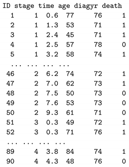
We use a publicly available larynx cancer dataset to illustrate the process of making survival time predictions. This dataset consists of records for 90 male larynx cancer patients, each with five variables: the stage of the disease (stage: 1, 2, 3, 4), the time to death or the duration of on-study time in months (time), the age at the diagnosis of larynx cancer (age), the year of diagnosis of larynx cancer (diagyr), and a death indicator (death: 0 = alive, 1 = dead). We added a new variable ID into the dataset and changed the variable name delta to death. The dataset can be downloaded from https://vincentarelbundock.github.io/Rdatasets/datasets.html.

The larynx cancer data are structured as follows:

We used two predictor variables to make survival time predictions: the stage of the disease and the age at the diagnosis of larynx cancer. Since the “stage” is a categorical variable, we created three dummy variables for stages 2, 3, and 4, with stage 1 as the default reference group. The survival probability of patients at various stages and time intervals can be observed in the following Kaplan–Meier plot (Figure 1):

The Weibull AFT model can be expressed as follows:

$$log\left(T\right)={\beta }_0+{\beta }_1\ast stage2+{\beta }_2\ast stage3+{\beta }_3\ast stage4+{\beta }_4\ast age+\sigma ϵϵ\sim G(0,1)$$

Most statistical software, such as R, can be used to run the Weibull regression model. In R, we can use the following code:

library(survival)

larynx<-read.csv("D:/larynx.csv")

wr <- survreg(Surv(time, death) ~ factor(stage) + age,

data = larynx,dist="w")

summary(wr)

The following results were obtained from the model:

Call:
survreg(formula = Surv(time, death) ~ factor(stage) + age, data = larynx,
dist = "w")
	Value	Std. Error	z	p
(Intercept)	3.5288	0.9041	3.903	9.50e-05
factor(stage)2	-0.1477	0.4076	-0.362	7.17e-01
factor(stage)3	-0.5866	0.3199	-1.833	6.68e-02
factor(stage)4	-1.5441	0.3633	-4.251	2.13e-05
age	-0.0175	0.0128	-1.367	1.72e-01
Log(scale)	-0.1223	0.1225	-0.999	3.18e-01
Scale = 0.885
Weibull distribution
Loglik(model) = -141.4		Loglik(intercept only) = -151.1
Chisq= 19.37 on 4 degrees of freedom, p = 0.00066
Number of Newton-Raphson Iterations: 5
n = 90

Suppose we want to predict the survival time for a patient with ID = 46, who is at larynx cancer stage 2 and is 74 years old. We can use the following equations:

1.

To calculate the mean time to failure (MTTF):

$$\begin{array}{cc}\hfill MTT{F}_{46}& =\widehat{E\left(t_{46}\right)}=exp\left({\mathit{x}}_{\mathit{i}}^{\prime }\widehat{\mathit{\beta }}\right)\mathsf{\Gamma }(\widehat{\sigma }+1)\hfill \\ & =exp(3.5288-0.1477\ast 1-0.5866\ast 0-1.5441\ast 0-0.0175\ast 74)\ast \mathsf{\Gamma }\left(1.885\right)\hfill \\ & =7.7\left(months\right)\hfill \end{array}$$

2.

To calculate the median survival time:

$$\begin{array}{cc}\hfill Media{n}_{46}& ={(log2)}^{\widehat{\sigma }}exp\left({\mathit{x}}_{\mathit{i}}^{\prime }\widehat{\mathit{\beta }}\right)\hfill \\ & =log{\left(2\right)}^{0.885}exp(3.5288-0.1477\ast 1-0.5866\ast 0-1.5441\ast 0-0.0175\ast 74)\hfill \\ & =5.8\left(\mathrm{months}\right)\hfill \end{array}$$

3.

To calculate the minimum prediction error survival time (MPET) using Equation (26) with a fixed k = 2:

$$\begin{array}{cc}\hfill MPE{T}_{46}& ={\left[\frac{\frac{2}{\sigma }log\left(k\right)}{k^{\frac{1}{\sigma }}-k^{-\frac{1}{\sigma }}}\right]}^{\sigma }exp\left({\mathit{x}}^{\prime }\mathit{\beta }\right)\hfill \\ & ={\left[\frac{\frac{2}{\sigma }log\left(k\right)}{2^{\frac{1}{0.885}}-k^{-\frac{1}{0.885}}}\right]}^{0.885}\ast exp(3.5288-0.1477\ast 1-0.5866\ast 0-1.5441\ast 0-0.0175\ast 74)\hfill \\ & =7.4\left(\mathrm{months}\right)\hfill \end{array}$$

It seems that these prediction methods yield results quite close to the real survival time of patient ID = 46, which was 6.2 months.

10. Calculating the 95% Confidence Interval of the Predicted Time

First, we used Equation (21) to calculate the standard error of the survival time:

$$\begin{array}{cc}\hfill SE& ={\left\{{\left(\begin{array}{c}\frac{\partial \widehat{E\left(t_i\right)}}{\partial \widehat{\mathit{\beta }}}\\ \frac{\partial \widehat{E\left(t_i\right)}}{\partial \widehat{\sigma }}\end{array}\right)}^t{\mathsf{\Sigma }}_{\widehat{\sigma }\widehat{\mathit{\beta }}}\left(\begin{array}{c}\frac{\partial \widehat{E\left(t_i\right)}}{\partial \widehat{\mathit{\beta }}}\\ \frac{\partial \widehat{E\left(t_i\right)}}{\partial \widehat{\sigma }}\end{array}\right)\right\}}^{\frac{1}{2}}\hfill \\ & ={\left\{{\left(\begin{array}{c}\frac{\partial {(log2)}^{\widehat{\sigma }}exp\left({\mathit{x}}_{\mathit{i}}^{\prime }\widehat{\mathit{\beta }}\right)}{\partial \widehat{\mathit{\beta }}}\\ \frac{\partial {(log2)}^{\widehat{\sigma }}exp\left({\mathit{x}}_{\mathit{i}}^{\prime }\widehat{\mathit{\beta }}\right)}{\partial \widehat{\sigma }}\end{array}\right)}^t{\mathsf{\Sigma }}_{\widehat{\sigma }\widehat{\mathit{\beta }}}\left(\begin{array}{c}\frac{\partial {(log2)}^{\widehat{\sigma }}exp\left({\mathit{x}}_{\mathit{i}}^{\prime }\widehat{\mathit{\beta }}\right)}{\partial \widehat{\mathit{\beta }}}\\ \frac{\partial {(log2)}^{\widehat{\sigma }}exp\left({\mathit{x}}_{\mathit{i}}^{\prime }\widehat{\mathit{\beta }}\right)}{\partial \widehat{\sigma }}\end{array}\right)\right\}}^{\frac{1}{2}}\hfill \\ & ={\left\{{\left(\begin{array}{c}{(log2)}^{\widehat{\sigma }}exp\left({\mathit{x}}^{\prime }\widehat{\mathit{\beta }}\right)\hfill \\ {(log2)}^{\widehat{\sigma }}exp\left({\mathit{x}}^{\prime }\widehat{\mathit{\beta }}\right)\ast stage2\hfill \\ {(log2)}^{\widehat{\sigma }}exp\left({\mathit{x}}^{\prime }\widehat{\mathit{\beta }}\right)\ast stage3\hfill \\ {(log2)}^{\widehat{\sigma }}exp\left({\mathit{x}}^{\prime }\widehat{\mathit{\beta }}\right)\ast stage4\hfill \\ {(log2)}^{\widehat{\sigma }}exp\left({\mathit{x}}^{\prime }\widehat{\mathit{\beta }}\right)\ast age\hfill \\ {(log2)}^{\widehat{\sigma }}log(log2)exp\left({\mathit{x}}^{\prime }\widehat{\mathit{\beta }}\right)\hfill \end{array}\right)}^t{\mathsf{\Sigma }}_{\widehat{\sigma }\widehat{\mathit{\beta }}}\left(\begin{array}{c}{(log2)}^{\widehat{\sigma }}exp\left({\mathit{x}}^{\prime }\widehat{\mathit{\beta }}\right)\hfill \\ {(log2)}^{\widehat{\sigma }}exp\left({\mathit{x}}^{\prime }\widehat{\mathit{\beta }}\right)\ast stage2\hfill \\ {(log2)}^{\widehat{\sigma }}exp\left({\mathit{x}}^{\prime }\widehat{\mathit{\beta }}\right)\ast stage3\hfill \\ {(log2)}^{\widehat{\sigma }}exp\left({\mathit{x}}^{\prime }\widehat{\mathit{\beta }}\right)\ast stage4\hfill \\ {(log2)}^{\widehat{\sigma }}exp\left({\mathit{x}}^{\prime }\widehat{\mathit{\beta }}\right)\ast age\hfill \\ {(log2)}^{\widehat{\sigma }}log(log2)exp\left({\mathit{x}}^{\prime }\widehat{\mathit{\beta }}\right)\hfill \end{array}\right)\right\}}^{\frac{1}{2}}\hfill \end{array}$$

(26)

The variance–covariance matrix ${\mathsf{\Sigma }}_{\widehat{\sigma }\widehat{\mathit{\beta }}}$ can be calculated by the observed Fisher information of the Weibull AFT model. In most statistical software, this variance–covariance matrix can be computed directly. In R, we used the following R code to obtain the ${\mathsf{\Sigma }}_{\widehat{\sigma }\widehat{\mathit{\beta }}}$matrix:

wr$var

which produces the following:

	(Intercept)	stage2	stage3	stage4	age	Log(scale)
(Intercept)	0.817	-0.09049	-0.08479	-0.0444	-0.01114	0.02591
stage2	-0.090	0.16611	0.05319	0.0507	0.00057	0.00016
stage3	-0.085	0.05319	0.10237	0.0567	0.00042	-0.00731
stage4	-0.044	0.05068	0.05668	0.1320	-0.00020	-0.01070
age	-0.011	0.00057	0.00042	-0.0002	0.00016	-0.00026
Log(scale)	0.026	0.00016	-0.00731	-0.0107	-0.00026	0.01501

Note that in the results above, the last row represents the log(scale), denoted as $log\left(\widehat{\sigma }\right)$, and what we obtained is the covariance of $\widehat{\beta }$s and $log\left(\widehat{\sigma }\right)$. For ${\mathsf{\Sigma }}_{\widehat{\sigma }\widehat{\mathit{\beta }}}$, we needed to change $log\left(\widehat{\sigma }\right)$ back to $\widehat{\sigma }$. Some extra calculations were needed. To make this adjustment, we can refer to the formulas found on page 401 of John Klein’s book [10]. Our calculations were:

$$\begin{array}{cc}\hfill & Cov({\beta }_0,\sigma ,)=Cov({\beta }_0,e^{log\left(\sigma \right)})=Cov({\beta }_0,log\left(\sigma \right))\ast \sigma =0.02292735\hfill \\ & Cov({\beta }_1,\sigma ,)=Cov({\beta }_1,e^{log\left(\sigma \right)})=Cov({\beta }_1,log\left(\sigma \right))\ast \sigma =0.0001403178\hfill \\ & Cov({\beta }_2,\sigma ,)=Cov({\beta }_2,e^{log\left(\sigma \right)})=Cov({\beta }_2,log\left(\sigma \right))\ast \sigma -0.006469443\hfill \\ & Cov({\beta }_3,\sigma ,)=Cov({\beta }_3,e^{log\left(\sigma \right)})=Cov({\beta }_3,log\left(\sigma \right))\ast \sigma =-0.009470604\hfill \\ & Cov({\beta }_4,\sigma ,)=Cov({\beta }_4,e^{log\left(\sigma \right)})=Cov({\beta }_4,log\left(\sigma \right))\ast \sigma =-0.0002297781\hfill \\ & Cov\left(\sigma \right)=Cov\left(e^{log\left(\sigma \right)}\right)={\left(e^{log\left(\sigma \right)}\right)}^{2}Cov(log\left(\sigma \right))={\sigma }^{2}Var\left(log\left(\sigma \right)\right)=0.0117501\hfill \end{array}$$

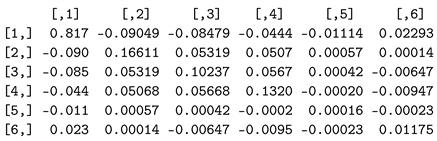
We replaced the last row of our variance–covariance matrix from R with these six values: which is the ${\mathsf{\Sigma }}_{\widehat{\sigma }\widehat{\mathit{\beta }}}$ matrix needed to calculate the standard error in Equation (26).

If we use SAS software (SAS (SAS Institute Inc., Cary, NC, USA)), we can directly obtain the variance–covariance matrix of $\widehat{\mathit{\beta }}$ and $\widehat{\sigma }$ by using the following statements:

proc lifereg data=larynx order=data COVOUT outest=est;

class stage;

model time∗death(0)=stage age/dist=weibull;

run;

proc print data=est;

run;

The column vector on the right side of ${\mathsf{\Sigma }}_{\widehat{\sigma }\widehat{\mathit{\beta }}}$ in Equation (26) can be calculated as follows:

$$\begin{array}{c}\left(\begin{array}{c}{(log2)}^{\widehat{\sigma }}exp\left({\mathit{x}}^{\prime }\widehat{\mathit{\beta }}\right)\hfill \\ {(log2)}^{\widehat{\sigma }}exp\left({\mathit{x}}^{\prime }\widehat{\mathit{\beta }}\right)\ast stage2\hfill \\ {(log2)}^{\widehat{\sigma }}exp\left({\mathit{x}}^{\prime }\widehat{\mathit{\beta }}\right)\ast stage3\hfill \\ {(log2)}^{\widehat{\sigma }}exp\left({\mathit{x}}^{\prime }\widehat{\mathit{\beta }}\right)\ast stage4\hfill \\ {(log2)}^{\widehat{\sigma }}exp\left({\mathit{x}}^{\prime }\widehat{\mathit{\beta }}\right)\ast age\hfill \\ {(log2)}^{\widehat{\sigma }}log(log2)exp\left({\mathit{x}}^{\prime }\widehat{\mathit{\beta }}\right)\hfill \end{array}\right)\hfill \\ =\left(\begin{array}{c}{\left(\log 2\right)}^{0.885}\exp (3.5288-0.1477\ast 1-0.5866\ast 0-1.5441\ast 0-0.0175\ast 74)\hfill \\ {\left(\log 2\right)}^{0.885}\exp (3.5288-0.1477\ast 1-0.5866\ast 0-1.5441\ast 0-0.0175\ast 74\ast 1)\hfill \\ {\left(\log 2\right)}^{0.885}\exp (3.5288-0.1477\ast 1-0.5866\ast 0-1.5441\ast 0-0.0175\ast 74\ast 0)\hfill \\ {\left(\log 2\right)}^{0.885}a\exp (3.5288-0.1477\ast 1-0.5866\ast 0-1.5441\ast 0-0.0175\ast 74\ast 0)\hfill \\ {\left(\log 2\right)}^{0.885}\exp (3.5288-0.1477\ast 1-0.5866\ast 0-1.5441\ast 0-0.0175\ast 74\ast 74)\hfill \\ {\left(\log 2\right)}^{0.885}\log \log \left(\log 2\right)\exp (3.5288-0.1477\ast 1-0.5866\ast 0-1.5441\ast 0-0.0175\ast 74)\hfill \end{array}\right)\hfill \\ =\left(\begin{array}{c}\hfill 5.8383\hfill \\ \hfill 5.8383\hfill \\ \hfill 0\hfill \\ \hfill 0\hfill \\ \hfill 432.03\hfill \\ \mathrm{-7.7915}\hfill \end{array}\right)\hfill \end{array}$$

Now, with all the necessary components in place, we can calculate the standard error of the median survival time:

$$\begin{array}{cc}\hfill SE& ={\left\{{\left(\begin{array}{c}5.8383\\ 5.8383\\ 0\\ 0\\ 432.03\\ -7.7915\end{array}\right)}^t\left(\begin{array}{cccccc}0.817& -0.0905& -0.0848& -0.0444& -0.0111& 0.0229\\ -0.090& 0.1661& 0.0532& 0.0507& 0.00057& 0.00014\\ -0.0859& 0.0532& 0.1024& 0.0567& 0.00042& -0.0065\\ -0.044& 0.0507& 0.0567& 0.1320& -0.00020& -0.0095\\ -0.011& 0.00057& 0.0004& -0.00020& 0.00016& -0.00023\\ 0.023& 0.00014& -0.0065& -0.0095& -0.00023& 0.01175\end{array}\right)\left(\begin{array}{c}5.8383\\ 5.8383\\ 0\\ 0\\ 432.03\\ -7.7915\end{array}\right)\right\}}^{\frac{1}{2}}\hfill \\ & =2.156133\hfill \end{array}$$

This calculation yields a standard error of approximately 2.156133. Consequently, the 95% confidence interval for the median survival time is given by:

$$95\%CI:(5.83-1.96\ast 2.16<Media{n}_{46}<5.83+1.96\ast 2.16)=(1.60\mathrm{to}10.01)\mathrm{months}.$$

which means we are $95\%$ confident that the survival time will be within 1.60 to 10.01 months. Alternatively, we can employ the built-in R function $predict$ to estimate the median survival time as follows:

Median46<-predict(wr, newdata=data.frame(stage=2,age=74),type="quantile",

p=0.5,se.fit=TRUE)

Median46

This results in:

$fit

5.838288

$se.fit

2.095133

The standard error differs slightly from our calculations because R uses Greenwood’s formula to calculate the standard error of the survival function [11].

Note that in R’s built-in $predict$ function for the Weibull AFT model, type = “response” calculates $exp\left({\mathit{x}}^{\prime }\widehat{\mathit{\beta }}\right)$ without considering $\mathsf{\Gamma }(1+\widehat{\sigma })$ and type = “lp” computes ${\mathit{x}}^{\prime }\widehat{\mathit{\beta }}$ only; thus, we should not use them to predict MTTF. Additionally, to the best of our knowledge, there is no available software for calculating the minimum prediction error survival time.

11. Assessing Point Prediction Accuracy

Henderson et al. [9], inspired by Parkes [12], introduced a simple approach to assess the accuracy of predicted survival times. Let t represent the observed survival time and p represent the predicted time. If $p/k\le t\le kp$, then the point prediction p is considered as “accurate”, otherwise, it is labeled as “inaccurate”.

Alternatively, Christakis and Lamont proposed a “33 percent rule” to measure accuracy. In that method, the observed time is divided by the predicted survival time, and a prediction is considered “accurate” if that quotient falls between 0.67 and 1.33. Values less than 0.67 or greater than 1.33 are categorized as “errors” [13]. That method is essentially equivalent to setting $k=3$ in Parkes’s method. For our accuracy assessment, we chose to use $k=2$. The accuracy rate was defined as the proportion of “accurate” predictions relative to the total sample size. The results are presented in

Table 1. Prediction results and accuracy (last digit in predicted time: 0, inaccurate; 1, accurate).

ID	Stage	Age	Death	Time	Median (95% CI)	MTTF	MPET
1	1	77	1	0.6	6.42 (3.16, 9.68), 0	8.47, 0	8.11, 0
2	1	53	1	1.3	9.77 (4.07, 15.46), 0	12.9, 0	12.34, 0
3	1	45	1	2.4	11.23 (3.07, 19.39), 0	14.84, 0	14.19, 0
4	1	57	0	2.5	9.11 (4.32, 13.89), 0	12.03, 0	11.5, 0
5	1	58	1	3.2	8.95 (4.36, 13.54), 0	11.82, 0	11.3, 0
6	1	51	0	3.2	10.11 (3.88, 16.34), 0	13.36, 0	12.78, 0
7	1	76	1	3.3	6.54 (3.29, 9.78), 1	8.62, 0	8.25, 0
8	1	63	0	3.3	8.2 (4.37, 12.03), 0	10.83, 0	10.36, 0
9	1	43	1	3.5	11.63 (2.72, 20.54), 0	15.36, 0	14.7, 0
10	1	60	1	3.5	8.64 (4.4, 12.89), 0	11.41, 0	10.91, 0
11	1	52	1	4	9.94 (3.98, 15.89), 0	13.13, 0	12.55, 0
12	1	63	1	4	8.2 (4.37, 12.03), 0	10.83, 0	10.36, 0
13	1	86	1	4.3	5.49 (1.96, 9.01), 1	7.24, 1	6.92, 1
14	1	48	0	4.5	10.66 (3.52, 17.79), 0	14.08, 0	13.47, 0
15	1	68	0	4.5	7.52 (4.12, 10.91), 1	9.92, 0	9.49, 0
16	1	81	1	5.3	5.99 (2.63, 9.34), 1	7.9, 1	7.56, 1
17	1	70	0	5.5	7.26 (3.96, 10.56), 1	9.58, 1	9.16, 1
18	1	58	0	5.9	8.95 (4.36, 13.54), 1	11.82, 0	11.3, 1
19	1	47	0	5.9	10.84 (3.38, 18.31), 1	14.33, 0	13.7, 0
20	1	75	1	6	6.65 (3.41, 9.89), 1	8.78, 1	8.39, 1
21	1	77	0	6.1	6.42 (3.16, 9.68), 1	8.47, 1	8.11, 1
22	1	64	0	6.2	8.06 (4.34, 11.77), 1	10.64, 1	10.18, 1
23	1	77	1	6.4	6.42 (3.16, 9.68), 1	8.47, 1	8.11, 1
24	1	67	1	6.5	7.65 (4.19, 11.1), 1	10.1, 1	9.66, 1
25	1	79	0	6.5	6.2 (2.9, 9.5), 1	8.18, 1	7.83, 1
26	1	61	0	6.7	8.49 (4.4, 12.58), 1	11.21, 1	10.73, 1
27	1	66	0	7	7.78 (4.25, 11.31), 1	10.27, 1	9.83, 1
28	1	68	1	7.4	7.52 (4.12, 10.91), 1	9.92, 1	9.49, 1
29	1	73	0	7.4	6.89 (3.65, 10.12), 1	9.09, 1	8.69, 1
30	1	56	0	8.1	9.27 (4.28, 14.26), 1	12.24, 1	11.71, 1
31	1	73	0	8.1	6.89 (3.65, 10.12), 1	9.09, 1	8.69, 1
32	1	58	0	9.6	8.95 (4.36, 13.54), 1	11.82, 1	11.3, 1
33	1	68	0	10.7	7.52 (4.12, 10.91), 1	9.92, 1	9.49, 1
34	2	86	1	0.2	4.73 (0.68, 8.78), 0	6.25, 0	5.97, 0
35	2	64	1	1.8	6.95 (2.37, 11.54), 0	9.18, 0	8.78, 0
36	2	63	1	2	7.07 (2.4, 11.75), 0	9.34, 0	8.93, 0
37	2	71	0	2.2	6.15 (1.96, 10.34), 0	8.12, 0	7.77, 0
38	2	67	0	2.6	6.6 (2.22, 10.97), 0	8.71, 0	8.33, 0
39	2	51	0	3.3	8.72 (2.28, 15.17), 0	11.52, 0	11.02, 0
40	2	70	1	3.6	6.26 (2.03, 10.49), 1	8.26, 0	7.9, 0
41	2	72	0	3.6	6.05 (1.89, 10.2), 1	7.98, 0	7.63, 0
42	2	81	1	4	5.17 (1.13, 9.21), 1	6.82, 1	6.52, 1
43	2	47	0	4.3	9.36 (1.98, 16.73), 0	12.36, 0	11.82, 0
44	2	64	0	4.3	6.95 (2.37, 11.54), 1	9.18, 0	8.78, 0
45	2	66	0	5	6.71 (2.28, 11.15), 1	8.86, 1	8.48, 1
46	2	74	1	6.2	5.84 (1.73, 9.94), 1	7.7, 1	7.37, 1
47	2	62	1	7	7.2 (2.43, 11.97), 1	9.51, 1	9.09, 1
48	2	50	0	7.5	8.88 (2.22, 15.54), 1	11.73, 1	11.22, 1
49	2	53	0	7.6	8.42 (2.38, 14.47), 1	11.13, 1	10.64, 1
50	2	61	0	9.3	7.33 (2.46, 12.2), 1	9.67, 1	9.25, 1
51	3	49	1	0.3	5.83 (2.41, 9.24), 0	7.69, 0	7.36, 0
52	3	71	1	0.3	3.97 (2.19, 5.75), 0	5.24, 0	5.01, 0
53	3	57	1	0.5	5.07 (2.68, 7.45), 0	6.69, 0	6.4, 0
54	3	79	1	0.7	3.45 (1.56, 5.34), 0	4.55, 0	4.35, 0
55	3	82	1	0.8	3.27 (1.32, 5.23), 0	4.32, 0	4.13, 0
56	3	49	1	1	5.83 (2.41, 9.24), 0	7.69, 0	7.36, 0
57	3	60	1	1.3	4.81 (2.68, 6.94), 0	6.35, 0	6.07, 0
58	3	64	1	1.6	4.48 (2.58, 6.39), 0	5.92, 0	5.66, 0
59	3	74	1	1.8	3.76 (1.96, 5.56), 0	4.97, 0	4.75, 0
60	3	72	1	1.9	3.9 (2.12, 5.68), 0	5.14, 0	4.92, 0
61	3	53	1	1.9	5.43 (2.6, 8.27), 0	7.17, 0	6.86, 0
62	3	54	1	3.2	5.34 (2.63, 8.05), 1	7.05, 0	6.74, 0
63	3	81	1	3.5	3.33 (1.4, 5.27), 1	4.39, 1	4.2, 1
64	3	52	0	3.7	5.53 (2.56, 8.49), 1	7.3, 1	6.98, 1
65	3	66	0	4.5	4.33 (2.49, 6.17), 1	5.71, 1	5.47, 1
66	3	54	0	4.8	5.34 (2.63, 8.05), 1	7.05, 1	6.74, 1
67	3	63	0	4.8	4.56 (2.61, 6.51), 1	6.02, 1	5.76, 1
68	3	59	1	5	4.89 (2.69, 7.1), 1	6.46, 1	6.18, 1
69	3	49	0	5	5.83 (2.41, 9.24), 1	7.69, 1	7.36, 1
70	3	69	0	5.1	4.11 (2.32, 5.89), 1	5.42, 1	5.19, 1
71	3	70	1	6.3	4.04 (2.26, 5.82), 1	5.33, 1	5.1, 1
72	3	65	1	6.4	4.41 (2.54, 6.27), 1	5.82, 1	5.56, 1
73	3	65	0	6.5	4.41 (2.54, 6.27), 1	5.82, 1	5.56, 1
74	3	68	1	7.8	4.18 (2.38, 5.98), 1	5.52, 1	5.28, 1
75	3	78	0	8	3.51 (1.64, 5.38), 0	4.63, 1	4.43, 1
76	3	69	0	9.3	4.11 (2.32, 5.89), 0	5.42, 1	5.19, 1
77	3	51	0	10.1	5.63 (2.52, 8.73), 1	7.43, 1	7.11, 1
78	4	65	1	0.1	1.69 (0.77, 2.61), 0	2.23, 0	2.14, 0
79	4	71	1	0.3	1.52 (0.7, 2.34), 0	2.01, 0	1.92, 0
80	4	76	1	0.4	1.4 (0.61, 2.18), 0	1.84, 0	1.76, 0
81	4	65	1	0.8	1.69 (0.77, 2.61), 0	2.23, 0	2.14, 0
82	4	78	1	0.8	1.35 (0.56, 2.13), 1	1.78, 0	1.7, 0
83	4	41	1	1	2.57 (0.3, 4.84), 0	3.4, 0	3.25, 0
84	4	68	1	1.5	1.6 (0.74, 2.47), 1	2.12, 1	2.03, 1
85	4	69	1	2	1.58 (0.73, 2.42), 1	2.08, 1	1.99, 1
86	4	62	1	2.3	1.78 (0.78, 2.79), 1	2.35, 1	2.25, 1
87	4	74	0	2.9	1.44 (0.65, 2.24), 0	1.91, 1	1.82, 1
88	4	71	1	3.6	1.52 (0.7, 2.34), 0	2.01, 1	1.92, 1
89	4	84	1	3.8	1.21 (0.42, 2.01), 0	1.6, 0	1.53, 0
90	4	48	0	4.3	2.28 (0.57, 3.99), 1	3.01, 1	2.87, 1
Accuracy rate (%)					55.6% (50/90)	50% (45/90)	51.1% (46/90)

.

12. Discussion

In this paper, we introduced how to use the Weibull AFT model to predict when an event will occur. We utilized mean survival time (mean time to failure time, mean time between failures), median survival time, and minimum prediction error survival time to make predictions about the time from the baseline to the event. We also assessed prediction accuracy using Parkes’s method. When we fixed $k=2$, the accuracy was 55.6% for the median, 50% for the MTTF, and 51.1% for the MPET. However, by setting $k=3$, as suggested by Christakis and Lamont, the accuracy rate increased to 77.8%, 66.7%, and 67.8%, respectively. It is worth noting that our sample size was relatively small, and we only used two predictors. With a larger sample and more predictors, the accuracy rate could potentially be even higher. If there are many covariates that could be included in the model, various variable selection methods, such as backward elimination, forward selection, stepwise selection, and all possible subset selection can be employed. These methods may incorporate different stopping rules, such as p-values, Akaike information criterion (AIC), Bayesian information criterion (BIC), and Mallows’s Cp statistic to construct clinical prediction models [14]. Additionally, in this sample, we did not observe that the MPET had a significantly better accuracy rate than the median survival time.

Parametric survival models offer advantages in predicting survival time compared to the semiparametric Cox regression model. The Cox regression model, which can be specified as $S_i\left(t\right|x_i)=S_0{\left(t\right)}^{exp\left({\mathit{x}}_{\mathit{i}}^{\prime }\mathit{\beta }\right)}$, cannot directly predict time. Instead, it requires first specifying a certain period of time and then calculates the probability of an event within that period of time. The lognormal model is an alternative parametric model that can be employed to fit survival data. However, it comes with a drawback—parametric survival models, including the lognormal model, necessitate stronger assumptions compared to semiparametric models. Other models, like the logistic regression model or neural network models, are typically utilized to model binary events, regardless of when those events occurred. Poisson regression models can also be applied to model survival data with count data types (0, 1, 2, 3, and so forth). Nevertheless, similar to the Cox model, a prespecified period of time is required to calculate the probability of an event. The choice of which model to use should be guided by the specific questions we aim to address and the type of available data [15].

Currently, most clinical prediction models calculate a patient’s probability of having or developing a specific disease or risk scores based on these probabilities [16]. However, providing a probability can be challenging to understand for the general population, and probability itself can be defined in various ways [17]. In practice, the time axis remains the most natural measure for both clinicians and patients. Predicting when an event will occur can offer a practical and concrete guide to clinicians and healthcare providers for managing their patients [18]. It can also assist families and patients in making suitable plans for the remaining lifespan.

In this paper, our intention was not to utilize the publicly available larynx cancer dataset for the development of an actual prediction tool. Rather, we employed the dataset to illustrate the application of statistical methods and evaluate point accuracy. Developing a real prediction tool would require a much larger dataset and rigorous internal and external validations. Readers interested in the steps to develop such a tool can refer to the book Clinical Prediction Models: A Practical Approach to Development, Validation, and Updating [19].