A Session-Based Recommendation Model That Integrates the Temporal Sequence of Session Interactions and the Global Distance-Awareness of Items with Graph Neural Networks

Abstract

In the session-based recommendation algorithm, a better class of methods is to model the complex interaction relationship within the session as a graph structure, and then use the graph neural network to capture the deep features of the item from it. However, most models do not deeply mine the effective information contained in the sequence temporal relationship, nor do they pay attention to the auxiliary contribution of the global distance in different sessions to the item representation. This paper proposes a session-based recommendation model that integrates the temporal sequence of session interactions and the global distance-awareness of items with graph neural networks (TSDA-GNN). First, according to all session sequences, a global graph, a session graph, and a feature graph are constructed. In the global graph, the average “spacing” between items is introduced to represent the association between two items in the global graph. In the session graph, the interaction timing of the item is combined as the weight information in the relationship matrix, and the connection matrix of the session graph is constructed, which can more accurately capture the association relationship between items. Finally, by fusing the feature information of the item, using a graph neural network can deeply mine user preferences hidden in the feature information of the item. The model can not only model the information transmission relationship between items in different sessions, but also further deeply mine the hidden information of global domain and item features. Multiple experiments on two benchmark datasets show that the model proposed in this paper achieves the best results in various indicators.

1. Introduction

1.1. Research Background

Recommendation systems mainly recommend the content that users are most likely to be interested in according to their historical interaction behavior, personalized preference settings, and other information, which can help users make effective choices that are beneficial to themselves among many diverse and complicated options. In addition, in practical applications, it is often difficult to obtain relevant information such as the user’s specific preference settings. For example, some users tend to use anonymous identities or browse related content directly on the website without accounts. Traditional recommendation methods are no longer applicable to the above application scenarios, so session-based recommendation technology was generated [1,2,3]. Session recommendation refers to the prediction of the next item that the user is most likely to buy or click based on the user’s historical session data [4].

For example, on the JD shopping website, the different products that users add to the shopping cart at one time constitute a session sequence, or the different news records that users browse on the internet for a continuous week are also a session sequence. In session recommendation, users are often anonymous, rather than a real, labeled user. The user’s behavior in the session is not only affected by the current session, but also by the item conversion relationship from other sessions. There is a lot of information to be mined [5].

This paper uses the natural advantage of graph neural network to capture and learn various complex association relationships from graph data, and studies how to use a graph neural network to model different levels of session item conversion relationships. A graph neural network session recommendation model (TSDA-GNN) that fuses sequence interaction timing and global distance awareness is proposed. We construct a global graph, session graph, and feature graph according to all session sequences, and use the powerful graph data learning and representation ability of a graph neural network to capture the conversion relationship between items from different levels. In the session graph, we use the interaction order of nodes as the weight information in the relationship matrix, and construct the connection matrix of the session graph, so as to model the conversion relationship between items more accurately.

We construct a global graph to capture the global item conversion by aggregating all the pairwise item conversions in the session. We also introduce the average “spacing” between items in the global graph as a measure of the association between two items. Then, we fuse the feature information of the item and use a graph neural network to deeply mine the hidden user preference information from the item features.

1.2. Related Work

Traditional session recommendation methods usually use data mining or machine learning techniques to mine the relevance within the session data, so as to carry out session recommendation [6]. For example, this kind of recommendation method based on frequent patterns and association rules first performs data mining of frequent patterns and association rules [7], then performs session matching and, finally, generates recommendation results. There are also session recommendation algorithms based on sequence pattern mining, such as using weighted sequence pattern mining related to users for recommendation, where the weight of each session sequence is calculated by its similarity with the historical interaction sequence of the target user [8]. There are also hybrid recommendation models that combine sequence pattern mining and collaborative filtering methods, so as to model the user’s dynamic short-term preferences and long-term preferences [9,10].

Another effective session recommendation method is the session recommendation method based on a Markov chain, which maps the current session to a Markov chain, and then predicts the next most likely interaction behavior of the user based on the previous behavior [11]. However, the model generally uses the last interaction record in the session sequence to predict the user’s next behavior, only using the local features in the session, and ignoring the role of context information in the session data.

Compared with traditional methods, deep learning can more effectively extract data features. Based on deep learning, recommendation algorithms train user interest preference representation through neural network models and use it to predict the next interaction [12,13,14]. For example, taking advantage of a recurrent neural network RNN in processing serialized data, Balazs Hidasi proposed the GRU4Rec model based on GRU (gated recurrent unit) [15], which only uses the user’s historical interaction data in the session for recommendation, and performs feature representation on the item sequence that the user clicked or browsed in a session.

Quadrana proposed a model using multi-layer recurrent neural networks [16], which considered the connection between different sessions, and used the feature representation of the previous session as the input of the next session modeling network. Li J proposed the NARM model [17], which integrated the ideas of an RNN model and attention mechanism and focused on both the user’s sequential behavior and interest preference. Leng and Yu proposed the HiCAR model [18], which divided the context information in the session into macro-level and micro-level contexts and used a multi-way hybrid strategy learning module to model the multi-feature interaction. LIU proposed the STAMP (Short-Term Attention/Memory Priority) model [19], which obtained the user’s long-term interest from the long-term memory of the session context and represented the user’s current interest by the last interacted item, effectively capturing the user’s interest preference information; however, this method did not consider the behavior information of the session sequence.

BACH used convolutional operations to extract complex local features and iteratively RNN models to extract the user’s long-term interest from the session sequence [20,21]. However, these model algorithms can only model the one-way transition relationship between items in the session and cannot deeply analyze and mine the transition relationship between other items in the session, which seriously affects the further effective improvement of the recommendation accuracy.

In recent years, due to the natural advantages of graph neural networks (GNNs) in solving graph structured data problems and their interpretability characteristics [22,23,24], they can naturally and explicitly encode the crucial collaborative signal to improve the user and item representations. A GNN can make excellent use of the structure of graphs to obtain the features of neighboring nodes in a natural and flexible way. The resulting node representations capture the low-frequency information of nodes, which is the commonality and similarity between the current node and its neighboring nodes. These commonalities and similarities are applicable to most recommendation tasks. GNNs have achieved remarkable success in recommender systems in the past few years. In academic research, a lot of works demonstrate that GNN-based models outperform previous methods [25,26]. Meanwhile, plenty of different forms of GNN are proposed and applied to various recommendation tasks, e.g., session-based recommendation, group recommendation, multimedia recommendation, and bundle recommendation. Researchers construct the session sequence data as graph-structured data and use GNNs to encode the complex node-to-node transition relationships in the session into embedding vectors, thereby learning the information embedding vectors of each interaction node. Shu et al. proposed the SR-GNN model based on a gated graph neural network [27], which uses a gated graph neural network to obtain the representation of each item, then uses soft attention to obtain the session representation to represent the user’s long-term preference and uses the last interaction item in the session to represent the user’s short-term preference, achieving better results than previous non-GNN models.

The GCSAN model uses a gated graph neural network and self-attention network to learn the local features [28], i.e., short-term interest, and global features, i.e., long-term interest, of the session, respectively. The TAGNN model first uses a gated graph neural network to learn the initial embedding vector of the item [29], and then constructs the target item representation for each item node vector obtained according to different target items, which is used to represent the user’s interest changes with different target items. Pan proposed the SGNN-HN model [30], which uses a star graph neural network (Star Graph Neural Networks) and adaptively selects embeddings from the item representation by using HighWay Networks, effectively alleviating the common overfitting problem in GNNs. Wang et al. proposed the GCE-GNN model [31], which constructs two kinds of graphs, a session graph and a global graph, learns the global-level item representation of the item in the global graph, learns the session-level item representation of the item in the session graph, and finally aggregates the two-layer item representation to obtain the interest representation of the session.

Gupta et al. proposed the CauSeR model [5], which uses causal relationships to create a causal reasoning framework for session recommendation, analyzes the sources of popularity bias that the model is prone to generate and model training in two stages, and effectively solves the problem of the long tail effect. However, these algorithms only use graph neural networks to learn the initial embedding vector of the item in the process of modeling and learn the item in the current session, and then use simple attention mechanism to obtain the user’s interest preference representation without fully considering some auxiliary information such as interaction timing and item features in the session, which has an auxiliary effect on the learning and calculation of the current session interest preference task. In contrast, our proposed model considers the item transfer relationship from the different dimensions of global graph, session graph, and item feature graph, which can more effectively predict the user’s interest preference.

2. The Proposed Model Algorithm

2.1. Model Structure Design

In the session recommendation task, different items are associated with each other due to various diverse and complex factors, and recommending to the current session user requires considering these complex associations between items. This paper constructs session data as a session graph, global graph, and feature graph, and models the historical session data from two perspectives of session and global neighborhood to obtain user preferences, which not only realizes the information transmission between different sessions, but also further deeply mines the hidden information in the global domain. This model also integrates the item feature information, fully mining the user preferences hidden in the item feature information. The overall architecture of the model is shown in Figure 1 below.

The input data in the model are all anonymous behavior sequences, and session recommendation predicts the next possible item of interest to the user based on these anonymous behavior sequences, thus generating effective recommendations. The session sequence data first need to be initialized after embedding, forming the initial embedding representation of the item, and then using the constructed global graph, session graph, feature graph, and using the powerful graph data learning and representation ability of graph neural networks, learning to capture the high-order embedding representation of the item. Among them, the item feature graph is based on the attributes and context feature information of the item itself to characterize the item, which implies the user’s interest preference. The model mainly consists of four modules: the item representation learning module at the session layer, the item representation learning module at the global domain layer, the aggregation module and the prediction scoring module.

1. The item representation learning module of the conversation layer. Based on the conversation sequence data, a conversation graph is constructed, and a GNN network model is used to learn the conversation layer item embedding representation in the current conversation. In the process of constructing the item connection matrix of the conversation graph, the interaction temporal information is considered, and the interaction temporal information is encoded to obtain the initial vector of the conversation node; secondly, in the item node learning representation of the conversation graph, the item feature information of the conversation itself is fully utilized, the domain set node information representation of the item is combined with its own feature information, and the item preference hidden in the item feature information is deeply mined by using the graph neural network.

2. The item representation learning module of the global domain layer. Based on all the conversation sequence data, a weighted global graph is constructed, which is a weighted graph that collects all the conversation sequence information. In the process of calculating the edge weights in the global graph, not only the frequency of each edge in all the conversations is considered, but also different weights are assigned to them according to the different “gaps” of the items in the conversation sequence. Then, by using an attention mechanism with a session-awareness function, based on the global graph structure, the embedding representation of the neighbor set of each node is aggregated to learn the global domain-level item embedding representation on all the conversations. Finally, using the graph neural network to deeply learn the item preference hidden in the item feature information by fusing the embedding representation vector of the item feature information and the embedding representation vector of the neighbor set, the item representation vector of the global domain layer is obtained.

3. The aggregation module. The vector representations of the conversation graph and the global neighborhood graph are aggregated to obtain the node representation and, finally, the attention mechanism is used to obtain the interest representation vector of the conversation.

4. The prediction score module. Based on the session interest representation obtained by the above method, the prediction scores of all the items are calculated and, finally, the final prediction results are output by sorting according to the score.

2.2. Item Representation Learning of the Conversation Layer

2.2.1. Constructing the Session Graph

The session graph is a weighted directed graph, denoted as $G_s$ = ($V_s, E_s$). We can capture the session-level item representation based on the item transition relationship in the current session sequence $S_{\mathrm{i}}=\left\{s_{\mathrm{I},1},s_{\mathrm{I},2},\dots ,s_{i,t}\right\}$. The node set $V_s$ represents the set of all items involved in all sessions, and the edge set $E_s$ is the representation of all item transition relationships in the session S that appear in $V_s$. The edge ($v_{i,t-1}, v_{i,t+1}$) indicates that in the session $S_i$, the user clicked on the item $v_{i,t-1}$ at time t, and then clicked on the item $v_{i,t+1}$ at the next time step.

Since the task of session recommendation is to recommend the next interaction item for the current session, in general, the last interaction item has a greater impact on the next interaction. Therefore, the closer the node is to the end of the session, the greater its influence on the session recommendation. So, in the process of constructing the session graph, we consider using the interaction sequence of nodes in the session as the weight information in the relationship matrix and assign different weights according to the interaction order position of nodes in the session. For example, for the session $S_1$ = {$v_1, v_2, v_3, v_4, v_3, v_1$}, which is shown in the following Figure 2.

According to the weighted session graph constructed above, the connection matrix $M_1$ of the session graph can be obtained as shown in the following Figure 3.

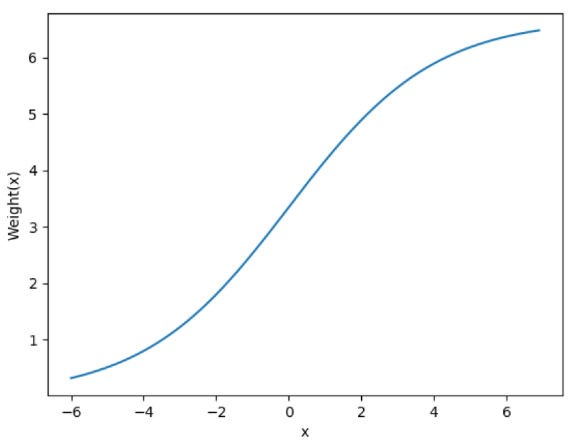
Because the actual session sequence data have different lengths, we normalize the weight information, and the specific normalization method is as follows:

$$Weight\left(x\right)=Mea{n}_S\times (\frac{1}{ 1+e^{-\frac{x}{2}}})$$

(1)

$Weight\left(x\right)$ represents the weight information in the connection matrix $M_1$, $x\in \left\{1,2,3,4, \dots ,n\right\}, Mea{n}_S$ represents the average session length of the session sequence data. According to the above weight information normalization formula, the final output weight size can be mapped to (0, $Mea{n}_S$). According to the average session length of the session data used in the experimental part of this paper, the weight information normalization curve is shown in the following Figure 4.

For the case where there are multiple repeated sequential interactions between two nodes in some session data, such as the edge ($v_{i,t-1}, v_{i,t+1}$) appearing multiple times, we take the weight value of the last occurrence. After normalizing the weight information according to the above, we obtain the standardized connection matrix $M_1^{\prime }$ of session $S_1$ as the following Figure 5.

The connection matrix $M_1^{\prime }$ serves as a crucial input feature for the following network model. It integrates its feature information with the parameter information of the graph neural network to propagate its own feature information to its neighboring nodes, and also receives feature information from its neighboring nodes. Therefore, it updates itself based on the aggregation of its own and neighboring information.

2.2.2. Item Representation Learning for the Session Graph

After constructing the weighted session graph as described above, we can use the graph neural network to encode the item representation vector and the item feature information representation vector and obtain the item embedding representation vector, which is a high-dimensional vector that represents the item feature information. Our model adopts the gated graph neural network (GGNN) to encode the item representation vector and the item feature information representation vector. The GGNN is a classic message passing model based on gated recurrent units (GRUs), which are specially designed for sequential problems. It can fix the number of iterations and use backpropagation algorithm directly in time to calculate the gradient. We use the standardized connection matrix $M_1^{\prime }$ constructed above to obtain the information of each node in GGNN. After the memory processing of GRU unit, we fuse the node information and optimize the information propagation process of GNN for nodes. The specific learning process is as follows:

$$a_{s,i}^t=M_1^{\prime } {[v_1^{t-1},v_2^{t-1},\dots ,v_n^{t-1}]}^{T}H+b$$

(2)

$$Z_{s,i}^t=\sigma \left(W_z{a}_{s,i}^t+U_z{v}_i^{t-1}\right)$$

(3)

$$R_{s,i}^t=\sigma \left(W_r{a}_{s,i}^t+U_{\mathrm{r}}{v}_i^{t-1}\right)$$

(4)

$${\tilde{h}}_{v_i}^t=\tanh \left(W_c{a}_{s,i}^t+P_c\left(R_{s,i}^t\odot v_i^{t-1}\right)\right)$$

(5)

$$h_{v_i}^t=\left(1-Z_{s,i}^t\right)\odot v_i^{t-1}+Z_{s,i}^t\odot {\tilde{h}}_{v_i}^t$$

(6)

In Equation (2), $a_{s,i}^t$ represents the generated item hidden vector and $M_1^{\prime }$ is the standardized conversational connection matrix obtained above. $Z_{s,i}^t$ and $R_{s,i}^t$ are the reset gate and update gate in the gated graph neural network. This part divides the hidden vector information into useful and useless information, and finally decides to retain or discard it through the sigmoid activation function. In Equations (5) and (6), $\odot$ represents multiplying elements one by one. We use the update gate and tanh function to calculate the candidate state and use the reset gate and the generated candidate state to obtain the vector representation of each node at time t, $h_{v_i}^t$. Similarly, for the item feature graph of the conversational sequence, we use the same method to construct the item feature representation vector of the corresponding session graph node, $h_{f_i}^t$. The calculation formula is as follows:

$$Z_{s,i}^{\prime t}=\sigma \left(W_{z^{\prime }}{a}_{s,i}^t+U_{z^{\prime }}{h}_{t-1}^F\right)$$

(7)

$${R\prime }_{s,i}^t=\sigma \left(W_{r^{\prime }}{a}_{s,i}^t+U_{r^{\prime }}{h}_{t-1}^F\right)$$

(8)

$${\widehat{h}}_t^F=\tanh \left(W_{h^F}{a}_{s,i}^t+U_{h^F}\left({r^{\prime }}_t\odot h_{t-1}^F\right)\right)$$

(9)

$$h_{f_i}^t=\left(1-{z^{\prime }}_t\right)\odot h_{f_i}^{t-1}+{z^{\prime }}_t\odot {\widehat{h}}_{f_i}^t$$

(10)

For each session graph and item feature graph, the gated graph neural network updates the nodes simultaneously. $a_{s,i}^t$ is used for information propagation between different nodes under the constraints given by the item connection matrix. Specifically, it extracts the latent vectors of the neighborhood and inputs them into the graph neural network as input data. Then, using the update gates $Z_{s,i}^t$, $Z_{s,i}^{\prime t}$ and the reset gates $R_{s,i}^t$, $R{\prime }_{s,i}^t$, they decide which information to retain and discard, respectively. After obtaining the representation vectors of the item $h_{v_i}^t$ and the item feature $h_{f_i}^t$ that we need, we concatenate $h_{v_i}^t$ and $h_{f_i}^t$ to obtain the final session-level item output vector ${\mathrm{h}}_{v_i}$, as shown in Equation (11):

$${\mathrm{h}}_{v_i}=concat\left(h_{v_i}^t,h_{f_i}^t\right)$$

(11)

2.3. Item Representation Learning Module for the Global Domain Layer

2.3.1. Constructing the Global Graph

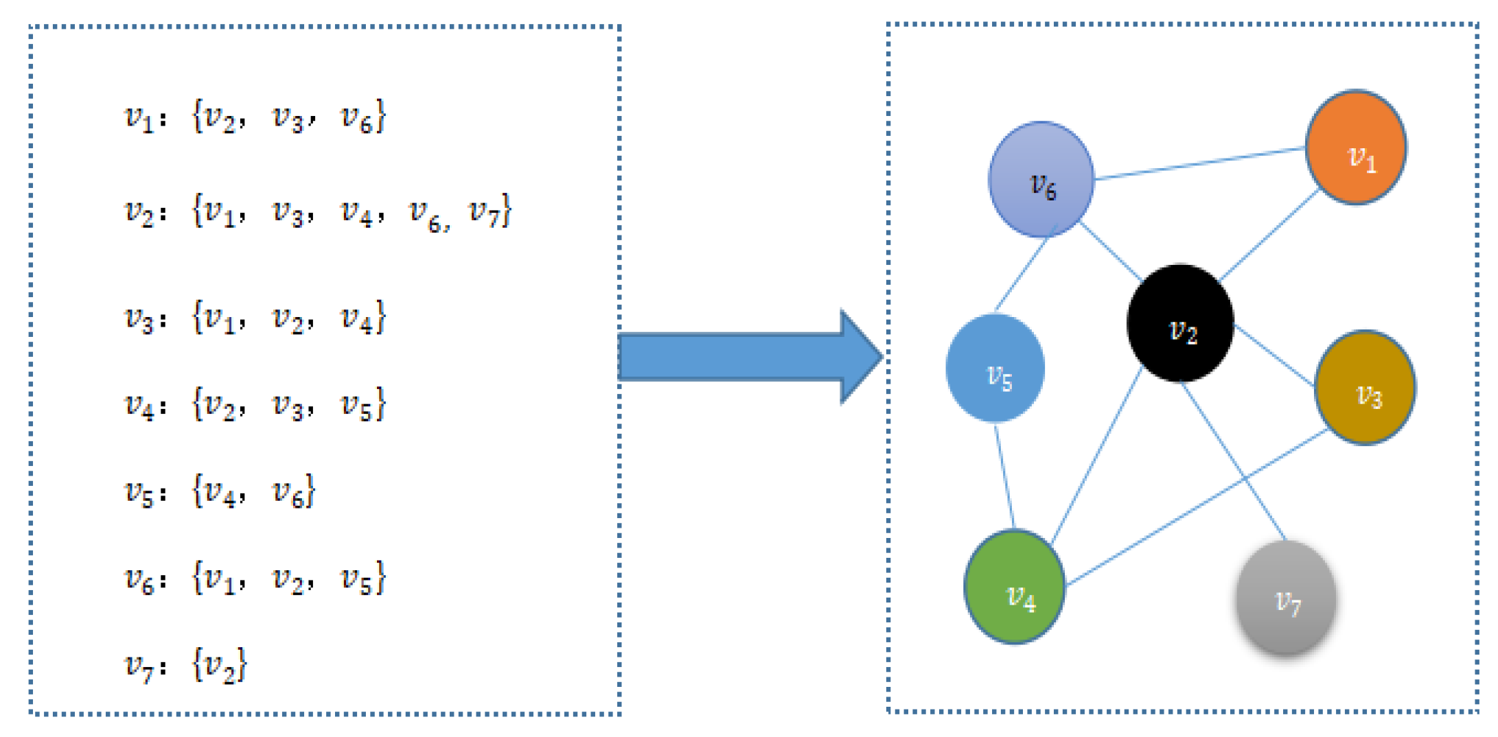
We consider the global item transition by aggregating all pairwise item transitions in the conversation. First, we introduce the concept of a neighborhood set here, and use the concept of a neighborhood set to establish the item transition relationship of the global sequence. A neighborhood is a topological structure on a set, that is, a nearby area. Let there be conversational sequences ${\mathrm{S}}_{\mathrm{p}}=\left\{{\mathrm{v}}_1^{\mathrm{p}},{ \mathrm{v}}_2^{\mathrm{p}},\dots ,{ \mathrm{v}}_{\mathrm{l}}^{\mathrm{p}}\right\},{ \mathrm{S}}_{\mathrm{q}}=\left\{{\mathrm{v}}_1^{\mathrm{q}},{ \mathrm{v}}_2^{\mathrm{q}},\dots ,{ \mathrm{v}}_{\mathrm{m}}^{\mathrm{q}}\right\}$, where l and m, respectively, represent the lengths of the conversational sequences ${\mathrm{S}}_{\mathrm{p}}$ and ${\mathrm{S}}_{\mathrm{q}}$; then, the representation formula of the neighborhood set is as follows:

$$\mathrm{N}\left({\mathrm{v}}_{\mathrm{i}}^{\mathrm{p}}\right)=\left\{{\mathrm{v}}_{\mathrm{j}}^{\mathrm{q}}\right|{\mathrm{v}}_{\mathrm{i}}^{\mathrm{p}}={\mathrm{v}}_{ \mathrm{i} \prime }^{\mathrm{q}}\in {\mathrm{S}}_{\mathrm{p}}\cap {\mathrm{S}}_{\mathrm{q}};{\mathrm{v}}_{\mathrm{i}}^{\mathrm{p}}\in {\mathrm{S}}_{\mathrm{q}};\mathrm{j}\in \left[{\mathrm{i}}^{\prime }-\mathsf{\epsilon },{\mathrm{i}}^{\prime }+\mathsf{\epsilon }\right];{\mathrm{S}}_{\mathrm{p}}\ne {\mathrm{S}}_{\mathrm{q}}\}$$

(12)

${\mathrm{i}}^{\prime }$ denotes the position of the item $v_i$ in ${\mathrm{S}}_{\mathrm{q}}$. $\mathsf{\epsilon }$ is the degree of the neighborhood, and if the degree is too large, it will introduce more noise information and some irrelevant item dependency relations.

Taking the following conversations $S_1$ = {$v_1, v_2, v_3, v_4, v_5, v_6$}, $S_2$ = {$v_1, v_3, v_4, v_2, v_6, v_1$}, and $S_3$ = {$v_6, v_2, v_7$} as an example, the constructed first-degree neighborhood set and neighborhood graph are as the following Figure 6.

The global graph $G_g=\left(V_g ,E_g\right)$ consists of a node set $V_g$ composed of items on all conversations, and an edge set $E_g=\left\{{\mathrm{e}}_{\mathrm{i},\mathrm{j}}\right|\left({\mathrm{v}}_{\mathrm{i}},{\mathrm{v}}_{\mathrm{j}}\right),{ \mathrm{v}}_{\mathrm{i}}\in {\mathrm{V}}_{\mathrm{g}}$, ${\mathrm{v}}_{\mathrm{j}}\in$N(${\mathrm{v}}_{\mathrm{i}}$)} that represents the transformation relationship between the current conversational item and its adjacent items in the global graph, where N(${\mathrm{v}}_{\mathrm{i}}$) is the neighbor set of the item ${\mathrm{v}}_{\mathrm{i}}$. The weight generation method of the edge set ${\mathrm{E}}_{\mathrm{g}}$ in the global graph is as follows. For each node, the weight of its adjacent edges consists of two parts. (1) The frequency of each edge in all conversations, because within a certain period of time, the more times two items are clicked sequentially in the same conversational sequence, the higher their similarity or relevance. The frequency weight of the edge is denoted as ${\mathrm{W}}_{\mathrm{ij}}^{\mathrm{f}}$. (2) According to the different “gaps” between two items, ${\mathrm{v}}_{\mathrm{I}}$ and ${\mathrm{v}}_{\mathrm{j}}$, in the conversational sequence, for example, the gap between items ${\mathrm{v}}_1$ and ${\mathrm{v}}_3$ in conversation ${\mathrm{v}}_3$ is 2, while the gap between items ${\mathrm{v}}_1$ and ${\mathrm{v}}_3$ in conversation ${\mathrm{S}}_2$ is 3. In the same conversational sequence, the shorter the “gap” between two items that are clicked sequentially, the stronger the relevance of these two interactions. Here, we use the average “gap” D of the edge in all sessions to represent the relevance of two items in the global graph. The “gap” weight of the edge is expressed as:

$${\mathrm{W}}_{\mathrm{ij}}^{\mathrm{as}}= \mathsf{\alpha }\times \left[\frac{\mathrm{D}}{\mathsf{\epsilon }}\right]$$

(13)

α is a coefficient, ε is a distance basic coefficient. Here, we consider the nodes which have a distance is within a certain range as having the same “gap” as the current node, so we use the rounded result as the final gap.

Therefore, the final weight of the edge, ${\mathrm{e}}_{\mathrm{I},\mathrm{j}}$, in the global graph is the sum of the frequency weight and the “gap” weight of the edge, expressed as follows:

$$W_{ij}={\mathrm{W}}_{\mathrm{ij} }^{\mathrm{f}}+{\mathrm{W}}_{\mathrm{ij}}^{\mathrm{AS}}$$

(14)

2.3.2. Item Representation Learning for the Global Graph

In the global graph, we use the attention mechanism to represent the different degrees of contribution of different items in the global graph to the representation of the current item. Secondly, we integrate the feature information of the item and use the graph neural network to deeply mine the item preference hidden in the item feature information. The ultimate goal of constructing the global neighborhood graph is to select useful information from the global sequence without introducing noise. We calculate the relevance of the current node and the neighborhood node on the neighborhood graph to represent the influence of the neighborhood set node on the prediction of the current node. The calculation formula of relevance $\omega \left(v_i,v_j\right)$ is as follows:

$$\omega \left(v_i,v_j\right)=q_1^{T}LeakyRelu(W_1[s\odot h_{v_j}||W_{ij}])$$

(15)

$h_{v_j}$ is the representation vector of node $v_j$, $W_1\in R^{\left(d+1\right)\left(d+1\right)}$ and $q_1\in R^{d+1}$ are trainable parameters, and $W_{ij}$ is the weight of edge ${\mathrm{e}}_{\mathrm{I},\mathrm{j}}$, which is the sum of the frequency weight and the “gap” weight of the edge. s is the feature vector of the current conversation S, which is the result of mean pooling over all nodes in conversation S, calculated as follows:

$$s=\frac{1}{l}{\sum }_{i=1}^l{h}_{v_i},\left(v_i\in S\right)$$

(16)

Equations (3)–(17) normalize the relevance and uses the softmax function to obtain the relevance probability of all neighborhood nodes of the current node:

$$\omega \left(v_i,v_j\right)=softmax\left(\frac{\exp \left(\omega \left(v_i,v_j\right)\right)}{{\sum }_{v_k\in N_{\alpha }\left(v_i\right)}\exp \left(\omega \left(v_i,v_k\right)\right)}\right)$$

(17)

Based on the relevance probability, we linearly combine the vector representations of each neighbor node in the neighbor set of the node, and obtain the vector representation of the neighbor node as follows:

$$h_{N_{\alpha }\left(v_i\right)}={\sum }_{v_j\in N_{\alpha }\left(v_i\right)}\omega \left(v_i,v_j\right)h_{v_j}$$

(18)

The representation of the item relies on both itself and its neighbor representations. Therefore, we aggregate the current node vector $h_{v_i}$ and the vector representation of its domain node $h_{N_{\alpha }\left(v_i\right)}$, and the implementation of the aggregation function is as follows:

$$h_{v_i}^g=relu(W_2[h_{v_i}\left|\right|h_{N_{\alpha }\left(v_i\right)}])$$

(19)

$W_2\in R^{d\ast 2d}$ is the transformation weight. We can use the aggregator to perform multiple aggregations and merge more relevant information into the representation of the target item. We represent the representation of a item in the k-th step as follows:

$$h_{v_i}^{g,\left(k\right)}=agg(h_{v_i}^{\left(k-1\right)},h_{N_{v_i}^g}^{\left(k-1\right)})$$

(20)

$h_{v_i}^{g,\left(k-1\right)}$ is the item representation generated by the previous term through the information propagation process, and its initial value $h_{v_i}^{g,\left(0\right)}$ is $h_{v_i}^g$. Therefore, the k-th order aggregated representation of the item is the result of integrating its initial embedding representation and the embedding representations of all its neighbors in the global graph, which makes the final item representation more efficient.

Finally, based on the item feature representation vector, ${\mathrm{h}}_{f_i}$, that we obtained earlier, we concatenate ${\mathrm{h}}_{f_i}$ and $h_{v_i}^g$ to obtain the final global domain layer item output vector h_$h_{v_i}^g$, as shown in the following formula:

$$h_{v_i}^g=concat\left({\mathrm{h}}_{f_i},h_{v_i}^{g,\left(k\right)}\right)$$

(21)

2.4. Aggregation Module

This subsection aggregates the vector representations of the session graph and the global graph to obtain the final representation of the node and, finally, obtains the sequential representation of the conversation. We think that the vector representations of the session graph and the global neighborhood graph are equally important. The final representation vector of each node $h_{v_i}^{\prime }$ is the result of adding the global domain-level representation and the session-level representation, where to avoid overfitting problems, we use the dropout method on both the global domain-level item representation and the session-level vector representation. The calculation formula is as follows:

$$h_{v_i}^{\prime }=dropout\left(h_{v_i}^g\right)+dropout\left(h_{v_i}\right)$$

(22)

Since the most recent interactions in a conversation can better represent the user’s current preferences, the items involved in these actions are more important for the recommendation results. Therefore, we incorporate both the reverse position information and the node item representation in the process of generating the conversational representation. We regard the reverse position information encoding as a bias vector and add different reverse position vectors to the item representation vectors at different positions in the conversational sequence. Then, we use soft attention to obtain the contribution of each node to the conversational sequence representation, and finally generate the final interest preference representation vector of the conversation. We follow the idea of the GCE-GNN model and use a position embedding matrix $P=\left\{P_1,P_2,\dots ,P_l\right\}$, where $P_i\in R^d$ is the position embedding vector, and l represents the length of the conversation. The specific calculation formula of the item embedding representation vector containing position information is as follows:

$$h_{p, i}=\tanh \left(W_3\left[h_{v_i^s}^{\prime }\parallel p_{l-i+1}\right]+b_3\right)$$

(23)

$h_{v_i^s}^{\prime }$ is the item representation vector of all items in the conversation obtained by inputting the conversational sequence $h_{v_i}^{\prime }$ into GNN, $W_3\in R^{d\ast 2d}$ and $b_3\in R^d$ are trainable parameters, and tanh is the activation function. Because the length of the conversational sequence is variable, we choose to use the reverse position embedding method, where the smaller the distance between the current item and the predicted item, the more important it is.

Similarly, we take the mean of the item representation vectors of all nodes in the conversational sequence output by the GNN to obtain the feature representation vector of the conversation as follows:

$$s^{\prime }=\frac{1}{l}{\sum }_{i=1}^l{h}_{v_i^s}^{\prime }$$

(24)

Then, we use soft attention to obtain the contribution weight of each node to the conversational sequence representation:

$${\beta }_i=q_2^{⊺}\sigma \left(W_4{h}_{p, i}+W_5{s}^{\prime }+b_4\right)$$

(25)

$W_{4,} W_5\in R^{d\ast 2d},$ and $b_4, b_5\in R^d$ are all trainable parameters.

Finally, by using the contribution weight of each node calculated above to linearly combine the item representations, we can obtain the final interest representation vector of the conversation as follows:

$$H_s={\sum }_{i=1}^l{\beta }_i{h}_{v_i^s}^{\prime }$$

(26)

The conversational representation, $H_s$, obtained by the above process integrates the node representations of the conversational level and the global domain level. In the process of constructing the session graph, it considers the interaction order of the nodes in the conversation as the weight information in the relation matrix and assigns different weights according to the interaction order of the nodes in the conversation. In the process of constructing the global graph, it not only considers the frequency of each edge in all conversations, but also assigns different contribution weights according to the different “gaps” between two items in the conversational sequence. Secondly, we use the graph neural network to deeply mine the item preference hidden in the item feature information, to model the relationship between items in the conversational data more effectively and to efficiently utilize the conversational information, which can more effectively predict the user’s interest preference.

2.5. Predictive Scoring Module

After obtaining the final interest representation vector, $H_s$, of session S by the calculation in the previous section, we can use it to make predictive recommendation. Based on the final interest representation vector of session S and the initial vectors of all items, we obtain the predicted score $y$ of the next item $v_i\in V$, which can be obtained by the following equation:

$${\widehat{y}}_i=Softmax\left(H_s{}^{⊺}{h}_{v_i}\right)$$

(27)

${\widehat{y}}_i$ represents the probability distribution of all recommended items. The recommendation problem is actually a classification problem, and the input predicted scores are also calculated by the Softmax function, so here we choose the cross-entropy loss function as the loss function. For a single sample, the cross-entropy loss function is calculated as follows:

$$L=-\left[ylog\widehat{y}+\left(1-y\right)\log \left(1-\widehat{y}\right)\right]$$

(28)

y is the actual score of the item and $\widehat{y}$ is the predicted score of the item. When $y=1$, $L=-log\widehat{y}$, the predicted score also tends to 1, and the trend of the loss function is consistent with the actual situation. When the actual score $y=0$, $L=-\log \left(1-\widehat{y}\right)$, the predicted score also approaches the actual score 0, and the loss function L is smaller; the predicted score tends to 1, and the loss function L is also larger. It can be seen that the loss function perfectly replicates the gap between the predicted score and the actual score. Moreover, the growth of the loss function is similar to the nature of the log function, which increases exponentially, which makes the predicted score output by the model after training closer to the actual score data. Therefore, the final loss function is as follows:

$$L=-{\displaystyle {\sum }_{i=1}^n}{y}_i\log \left({\widehat{y}}_i\right)+\left(1-y_i\right)\log \left(1-{\widehat{y}}_i\right)+\lambda {\left|\left|\theta \right|\right|}^2$$

(29)

$y_i$ is the actual score of the item, $v_i$, $\widehat{y}$ is the predicted score obtained, and the set of all learnable parameters $\mathsf{\theta }$ is used as a regularization term to prevent overfitting.

3. Model Experiment

3.1. Dataset and Preprocessing

We used two public datasets in the experiment: Diginetica and Tmall. The Diginetica dataset is from CIKM 2016, and was extracted from the search engine logs, recording the query words, product descriptions, user clicks, and purchases, etc. The Tmall dataset is from IJCAI-15, which is the anonymous user transaction data from the Tmall platform. Following the data processing method in reference [27], we first filtered out sessions with length 1, items with an occurrence less than 5, and items that only interacted in the test set. Then, we set the latest week’s sessions as the test set and the rest sessions as the training set. In addition, for a session $\mathrm{S}=\left\{s_1,s_2,\dots ,s_{\mathrm{n}}\right\}$, we generated sequences and corresponding labels by sequence splitting preprocessing, namely ([$s_1$], $s_2$), ([$s_1, s_2$], $s_3$), …, ([${\mathrm{s}}_1,{\mathrm{s}}_2$, …, ${\mathrm{s}}_{\mathrm{n}-1}$], $s_{\mathrm{n}}$). The summary statistics of the preprocessed datasets are shown in the following

Table 1. Summary statistics of the preprocessed datasets.

Dataset	Diginetica	Tmall
Clicks	982,961	818,479
Number of sessions in the training set	719,470	351,268
Number of sessions in the test set	60,858	25,898
Number of items	43,097	40,728
Average session length	5.12	6.69

.

3.2. Evaluation Indicators

In this paper, we used two common ranking-based evaluation indicators: P@N (precision) and MRR@N (mean reciprocal rank), where P@N represents the proportion of correctly recommended items in the top N items, and the larger the value of P, the better the recommendation effect of the model. The equation is as follows, where $n_{hit}$ represents the number of correctly predicted items.

$$P@N=\frac{n_{hit}}{n}$$

(30)

$n$ is the total number of items in the test dataset, M is the set of correctly recommended items in the top N recommended items, and the value of N is set to 20 in the experiment.

3.3. Comparison Models

In order to verify the performance of the model proposed in this paper, we used the following several recommendation models as comparison models in the experiment.

POP: This method recommends items based on their popularity in sessions, only recommending the N most frequent items in the session sequence.

Item-KNN: This method recommends items based on the similarity between the items in the current session and the items in other sessions, by calculating the similarity between the target item and the neighboring items and recommending items that have the same or similar attributes as the current item.

FPMC: This method is a hybrid model that combines matrix factorization and a Markov chain, which considers the temporal information of the sequence while capturing the user’s long-term preference.

GRU4Rec: This method is an RNN-based model that uses gated recurrent units (GRU) to model user sequences. It uses a ranking-based loss function and utilizes the item interaction information in the entire sequence.

NARM: This method is an improved model based on GRU4Rec, which uses an attention mechanism to capture the user’s main interest and pays more attention to the user’s main intention in the current session when recommending items.

STAMP: This method considers both the user’s long-term interest and short-term interest and is also a recommendation model that introduces an attention mechanism. The model captures the user’s general interest from the long-term memory of the session context, and also captures the user’s current interest based on the user’s last click short-term memory.

SR-GNN: This method obtains each item representation through a gated graph neural network, and then obtains session representation to represent user’s long-term interest through soft attention; at the same time, it takes the last item of the sequence as short-term interest and adopts a strategy that combines long-term interest and short-term interest, which can better predict the items that users may interact with next.

GC-SAN: This method replaces SRGNN’s attention mechanism with a self-attention mechanism, which adaptively captures the interaction and transition relationship of items through a self-attention mechanism. After multiple layers of the self-attention layer, it obtains user’s long-term interest.

TA-GNN: This model designs a target-aware attention mechanism to improve SRGNN’s attention mechanism. In this model, for each node vector of each item obtained, a target item representation is constructed to represent the user’s interest changing with different target items.

GCE-GNN: This model introduces global information into session recommendation model combined with graph neural network and adds relative position information of item nodes in session.

3.4. Parameter Settings

In order to ensure the comparability of the experiments, we set the dimension of the latent vector d to be fixed at 100, and the batch size of all models to be 100. We followed the method in references [14,16] and initialized all parameters with a Gaussian distribution with mean 0 and standard deviation 0.1. We used the Adam optimization algorithm that can automatically adjust the learning rate, with the initial learning rate set to 0.001, the learning rate decayed by 0.1 every 3 training epochs, and the number of training epochs set to 30. Referring to the previous experience of related model algorithms, the L2 norm penalty term was set to 10–5. Dropout was selected from {0.1, 0.2 … 0.9} for experiments and searched for the optimal effect, and 10% of the subsets were randomly selected from the training set for validation. The parameters of the global neighborhood graph were optimized by grid search, with the number of neighbors $\mathrm{N}\in$ {10,11,12,13,14,15}, and the order $\mathrm{k}\in$ {1,2}. The optimal parameter combination was N = 12, k = 2.

3.5. Analysis of the Results

We conducted comparative experiments on two datasets with the model proposed in this paper and the baseline models mentioned earlier. We used the statistical results of P@20 and MRR@20, and all the results are the average of 10 experimental results. The experimental results are shown in

Table 2. Comparison of experimental results on two datasets.

Dataset	Diginetica		Tmall
Metrics	P@20	MRR@20	P@20	MRR@20
POP	1.17	0.28	1.98	0.89
Item-KNN	35.72	11.55	9.12	3.30
FPMC	20.22	6.63	16.02	7.29
GRU4Rec	30.54	8.18	10.86	5.85
NARM	48.28	15.96	23.27	10.69
STAMP	46.52	15.13	26.42	13.35
SR-GNN	51.58	17.88	28.23	13.43
GC-SAN	42.85	13.56	12.25	6.06
TA-GNN	50.93	17.70	31.62	13.88
GCE-GNN	54.19	19.01	32.38	15.39
TSDA-GNN	55.21	19.45	33.29	15.82

below, from which it can be seen that the TSDA-GNN model proposed in this paper has the best performance on the tested indicators.

To visualize the data, Figure 7 and Figure 8 show the performance of different models on two datasets more vividly.

The experimental results show that the POP model, which only considers the popularity of items themselves and recommends items with a high occurrence frequency, is no longer suitable for the current massive data environment, and has the worst performance among all models. The FPMC model, which uses a first-order Markov chain and matrix factorization method, shows relatively good results. The Item-KNN model, which uses the similarity between items to make recommendations, achieves better performance, but it does not consider learning the user’s long-term interest representation based on their historical interaction behavior. The GRU4Rec model, which uses a recurrent neural network (RNN) to model all session data as a whole, learns the user’s long-term interest preference, and uses a gated recurrent unit (GRU) to model user sequences, can capture the hidden association relationship in session sequences well. Compared with traditional methods, GRU4Rec has greatly improved in performance indicators, which demonstrates that the session-based recommendation model based on deep learning is significantly better than traditional models. The NARM and STAMP models have further improved performance compared with GRU4Rec. The NARM model produces better results due to the addition of an attention mechanism, which shows that the attention mechanism can effectively learn the user’s main interest preference. The STAMP model also achieves superior performance by introducing the short-term interest of the session and combining it with the long-term interest, which leads to a better recommendation effect.

The experimental results of models such as SR-GNN, GC-SAN, etc., are better than those using RNN, which shows that using graph neural network to capture the transformation relationship between session items and using attention mechanism to obtain user’s interest preference is very effective in session recommendation. The excellent performance of the TA-GNN model shows that the target-aware attention learns different interest vector representations according to different target items, which improves the model’s effect in personalized recommendation. In the biased personalized recommendation, the target-aware attention is better than the traditional attention mechanism, while the soft attention is more suitable for general recommendation. The more superior experimental results of the GCE-GN model verify that building a global graph to introduce global domain information into the model further deepens the mining of hidden information in the global domain, which offers a certain help to improve the efficiency of recommendation model. Through these data, we can find that our proposed TSDA-GNN model has achieved better performance in these test indicators, which proves the effectiveness of our proposed model method. The main reasons why the performance of our proposed model algorithm has been effectively improved are as follows. On the one hand, our proposed TSDA-GNN model learns different levels of item embeddings from the session graph, global graph, and feature graph. On the other hand, in the process of constructing the session graph, we consider using the interaction sequence of nodes in the session as the weight information in the relationship matrix and assign different weights according to the interaction order position of nodes in the session. In this way, we can effectively integrate the position information of nodes in the session into their adjacency matrix, thereby distinguishing the importance of different positions in representing session interests. Finally, in the global graph, the average “spacing” between items is introduced to represent the association strength between two items in the global graph. This is because the shorter the “spacing” between two items being clicked in sequence, the stronger the correlation between these two interactions. In our proposed model, we also integrate the item’s feature information, which is useful for deeply mining the user preferences hidden in the item’s feature information.

3.6. Ablation Experiments

We conducted comparative experiments to verify whether the main components of the model are effective. We designed the following variant models for experiments:

(1) The TSDA-GNN-A model means that only the average “distance” between items is introduced in the global graph, and the feature information embedding vector and session-level item embedding vector of the item are fused to obtain the final global domain layer item embedding vector.

(2) The TSDA-GNN-B model means that only in the process of constructing the item connection matrix of the session graph is the interaction order information encoded to obtain the initial vector of the session node, and that the feature information embedding vector and session layer embedding vector of the item are fused to obtain the final session layer item embedding vector.

(3) The TSDA-GNN-F model means that in the process of learning the item embedding vectors of the session layer and the global domain layer, the fusion of item feature information is not considered. The results of the ablation experiments are shown as the

Table 3. Results of ablation experiments.

Dataset	Diginetica		Tmall
Metrics	P@20	MRR@20	P@20	MRR@20
TSDA-GNN-A	53.76	18.41	32.86	15.32
TSDA-GNN-B	54.86	19.24	32.82	15.39
TSDA-GNN-F	54.53	19.04	32.71	15.21
TSDA-GNN	55.21	19.45	33.29	15.82

:

The table above shows the experimental results of different comparison models. From the results, we can see that when the average “distance” between items in the global graph and the interaction order of items in the session graph are not considered as weight information in the relation matrix to construct the item connection matrix, the corresponding indicator values in the experimental results will decrease. Figure 9 and Figure 10 more vividly show the performance of each variant model on the dataset.

The comparison results above show that the TSDA-GNN-A model, in the process of calculating the session layer item embedding vector, calculates the adjacency matrix according to the directed session graph of the session data. We used the same method as in GC-SAN and other graph neural network-based recommendation model algorithms to construct it, and its experimental results have decreased significantly. This shows that using the interaction order of items in the session graph as weight information in the relation matrix to construct the item connection matrix can more effectively learn the association relationship between items.

The TSDA-GNN-B model, in the process of calculating the global domain layer item embedding vector, uses only the frequency of each edge in all sessions to represent the weight of adjacent edges in the domain. Its experimental results also have a certain decline, which shows that our combination of the average “distance” between items to characterize the association strength of two items has a certain auxiliary effect on learning the global domain layer item embedding representation.

According to the comparison results of TSDA-GNN-F and TSDA-GNN on two datasets, fusing item feature information plays a certain role in accurately learning user preferences. On Diginetica, compared with TSDA-GNN-F, TSDA-GNN’s value increased by 1.2 percentage points on P@20 and 2.1 percentage points on MRR@20. On the Tmall dataset, compared with TSDA-GNN-F, TSDA-GNN’s value increased by 1.7% and 3.8% on P@20 and MRR@20, respectively.

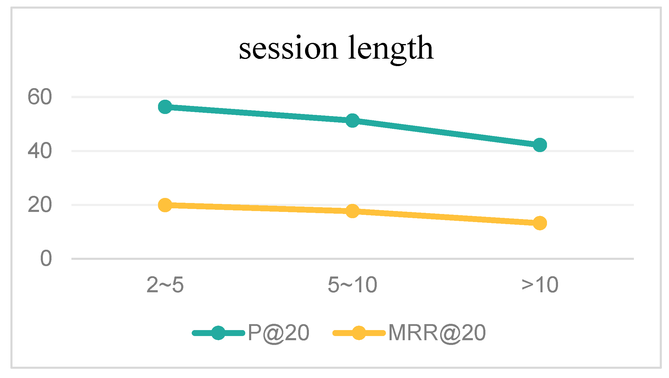
3.7. The Impact of Session Length

By classifying the Diginetica dataset according to session length, we removed all sessions with a length less than 2 during data preprocessing and divided the remaining session data into three parts: sessions with a length greater than 2 and less than 5; sessions with a length greater than 5 and less than 10; and sessions with a length greater than 10. We conducted relevant experiments under the same model parameters, and the experimental results are shown in the following Figure 11.

The experimental results show that the model performs best when the session length is between 2 and 5. However, as the session length increases, the model performance keeps decreasing, which indicates that a longer session length is not better. This may be due to the excessive session length, which adds more noise data to the session, or in other words, there are messy items in the data that disturb the unified modeling of user preferences. Multiple interactive items may have different preferences, which also leads to the inability of user interest preferences to be well represented in a unified way. For example, if in a session, after browsing notebook-related products, the user chooses to browse other products unrelated to notebooks, such as clothes, accessories, food, etc., this causes the model to fail to accurately capture the preference modeling of the session.

3.8. The Effect of Dropout Rate Setting

To prevent overfitting during the model training process, we adopted the dropout method, which mainly involves randomly discarding some neurons with a certain probability during the training process, while using all neurons for testing. In this experiment, we performed experiments on the Diginetica dataset with different values of dropout in {0.1, 0.2 … 0.9}, and the experimental results are shown in the following Figure 12.

From the experimental results in Figure 12, we can see that the change in the dropout parameter has a significant impact on the experimental performance on the Diginetica dataset and the Tmall dataset. From the figures, we can see that when the dropout rate is too small, overfitting occurs, and the model performance on both datasets is not very good. When the dropout rate is set to 0.4 on the Diginetica dataset and 0.6 on the Tmall dataset, the performance is optimal. However, when the dropout rate continues to increase, the model performance begins to decline, because the model struggles to learn useful information from limited data.

3.9. Experimental Results on Large Datasets

We conducted experimental tests on a larger dataset, Yoochoose, which are the data from the RecSys 2015 Challenge. Due to the large amount of preprocessed Yoochoose data, the session sequence closest to 1/16 of the test set time was selected as the training set, with a training set of 1,346,436 sessions and a testing set of 225,894 sessions. The final experimental results are shown in the Figure 13.

From the experimental results above, it can be seen that our model still exhibits some advantages when tested on a larger dataset. It could reveal insights into how the model performs with increased data volume.

3.10. Complexity Analysis

Due to the fact that the final training speed of the model is not only related to computational complexity, but also to other factors such as memory bandwidth, optimization level, and computational power of the processor, the following theoretical analysis was conducted on the complexity of the model.

If we assume that the session length is n and the hidden vector dimension is d, then the time complexity of initializing nodes in the out matrix is O$(n^2$d), and the time complexity of the graph convolution operation process is O$(n{d}^2$) for the GRU unit. If the number of items V is relatively large, the parameters of the model are mainly reflected in the embedding matrix of the items, and the parameter quantity is O$(Vd+d^2$). Comparative analysis with relevant algorithms shows that the model has little difference in spatial complexity. For the time complexity, the model proposed in this article does not have an advantage over the SRGNN model and the GC-SAN model, and there is not much difference in time complexity between them. Therefore, the main advantage of the TSDA-GNN model proposed in this paper is that the performance of our proposed model algorithm has been improved, under almost the same time and space complexity conditions.

4. Conclusions

This paper proposes a graph neural network sequence recommendation model, TSDA-GNN, that integrates sequence interaction timing and global distance awareness to address the problems existing in current session-based recommendation algorithms. The model builds a global graph, a session graph, and a feature graph based on all the session sequences, and integrates complex interaction information, user preferences, and item feature information in the session sequences in the form of graphs, thus obtaining embeddings with different dimensions. In the global graph, the average “distance” between items is introduced to indicate the relevance of two items in the global domain. In the session graph, the interaction order of items is used as the weight information in the relation matrix to construct the connection matrix of the session graph, which can more accurately capture the relevance between items. Finally, by aggregating the feature vectors of item feature information in the feature graph, the graph neural network is used to deeply mine the hidden item preferences in the item feature information. The final session representation vector integrates node information of different levels and dimensions, fully mines the item transfer relationship of different levels, and can more effectively predict user interest preferences. The experiments show that the model performs best on all indicators. Although the experiments verify that this model has certain advantages, there are still some shortcomings, such as after constructing the connection matrix of the session graph, this paper uses a gated graph neural network to encode and learn the representation vectors of item representation vector and item feature information representation vector. This experiment proves that the gated graph neural network indeed has superiority in dealing with session data. However, the deeper networks such as gated graph neural networks have more complex structures, a longer model training time, and a higher demand for computing resources such as GPU. In the future, we need to find effective networks that can reduce model training times. Furthermore, we think that the vector representations of the session graph and the global graph are equally important in this paper. In fact, their roles or importance may be different. So, we will try to consider distinguishing the different importance of the global graph and the session graph in future research work. In addition, we have not considered using graph enhancement and contrastive learning to improve the performance of the model, which is what we also need to study in the future.