
A Comparison of the Use of Artificial Intelligence Methods in the Estimation of Thermoluminescence Glow Curves

Abstract
:1. Introduction
2. Related Work
3. Material and Methods
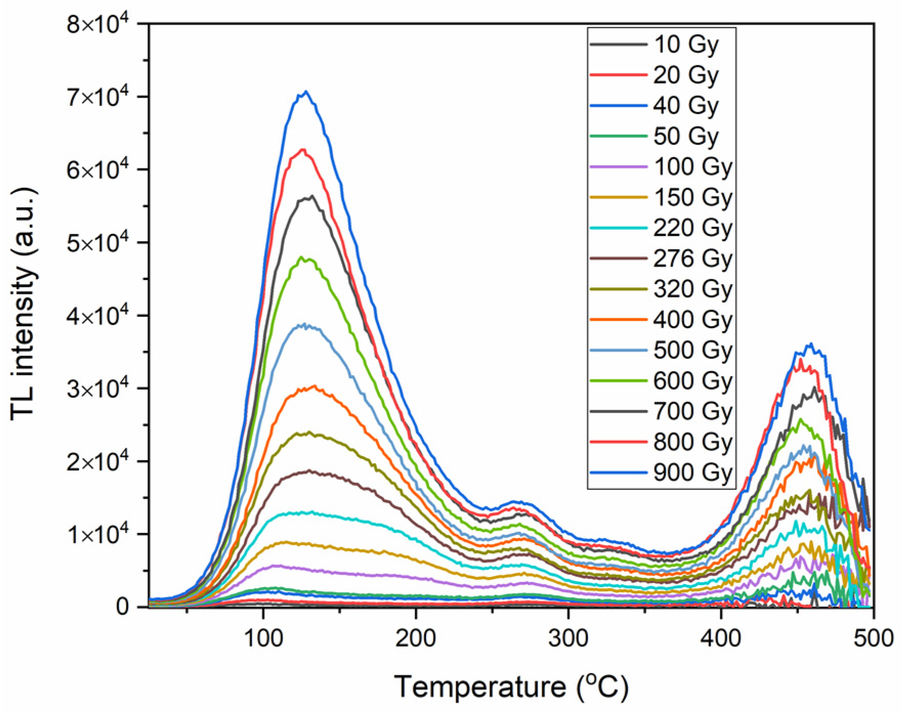
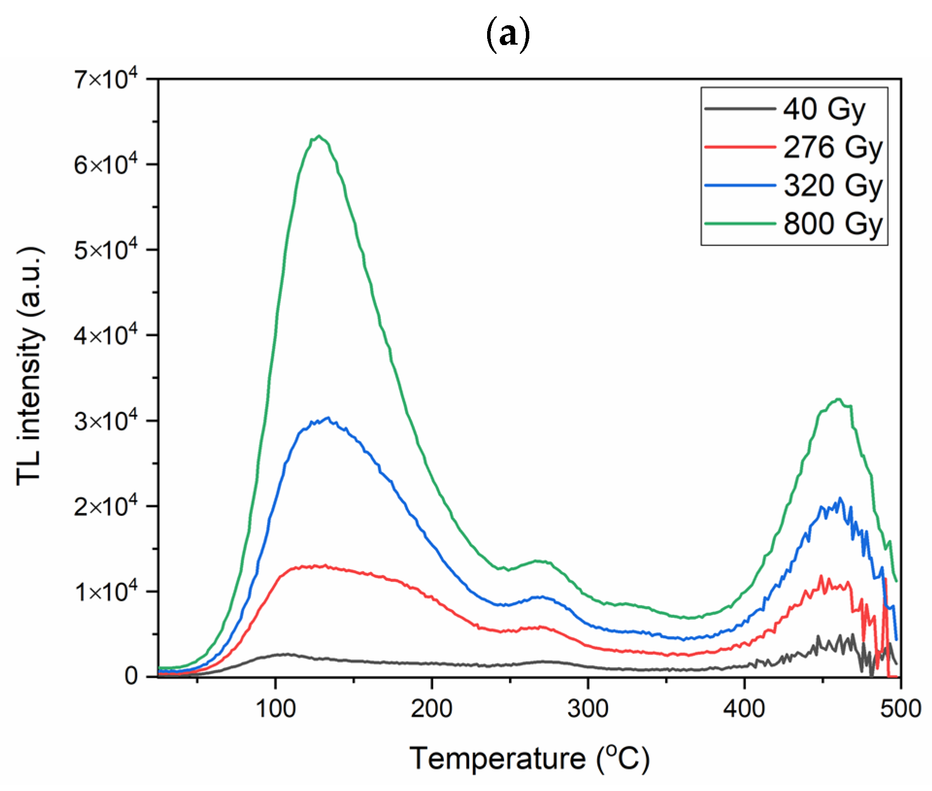
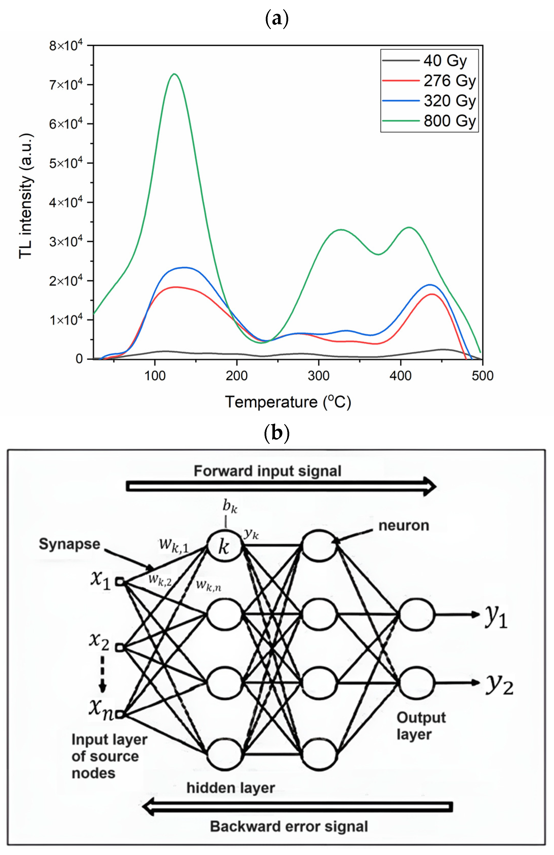
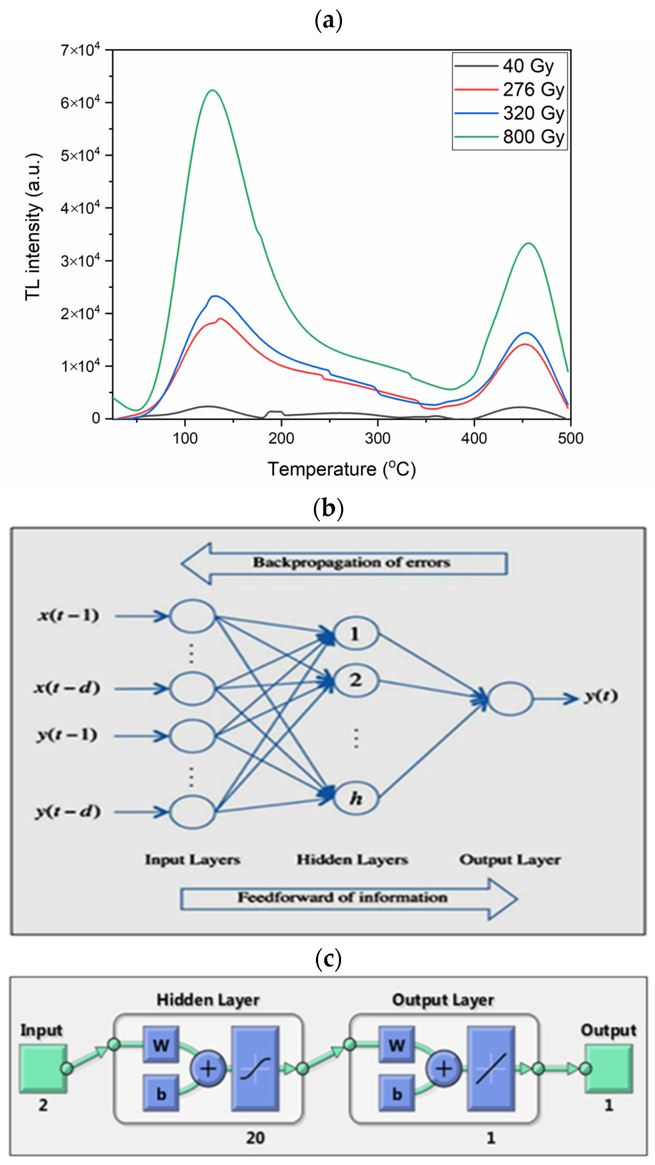
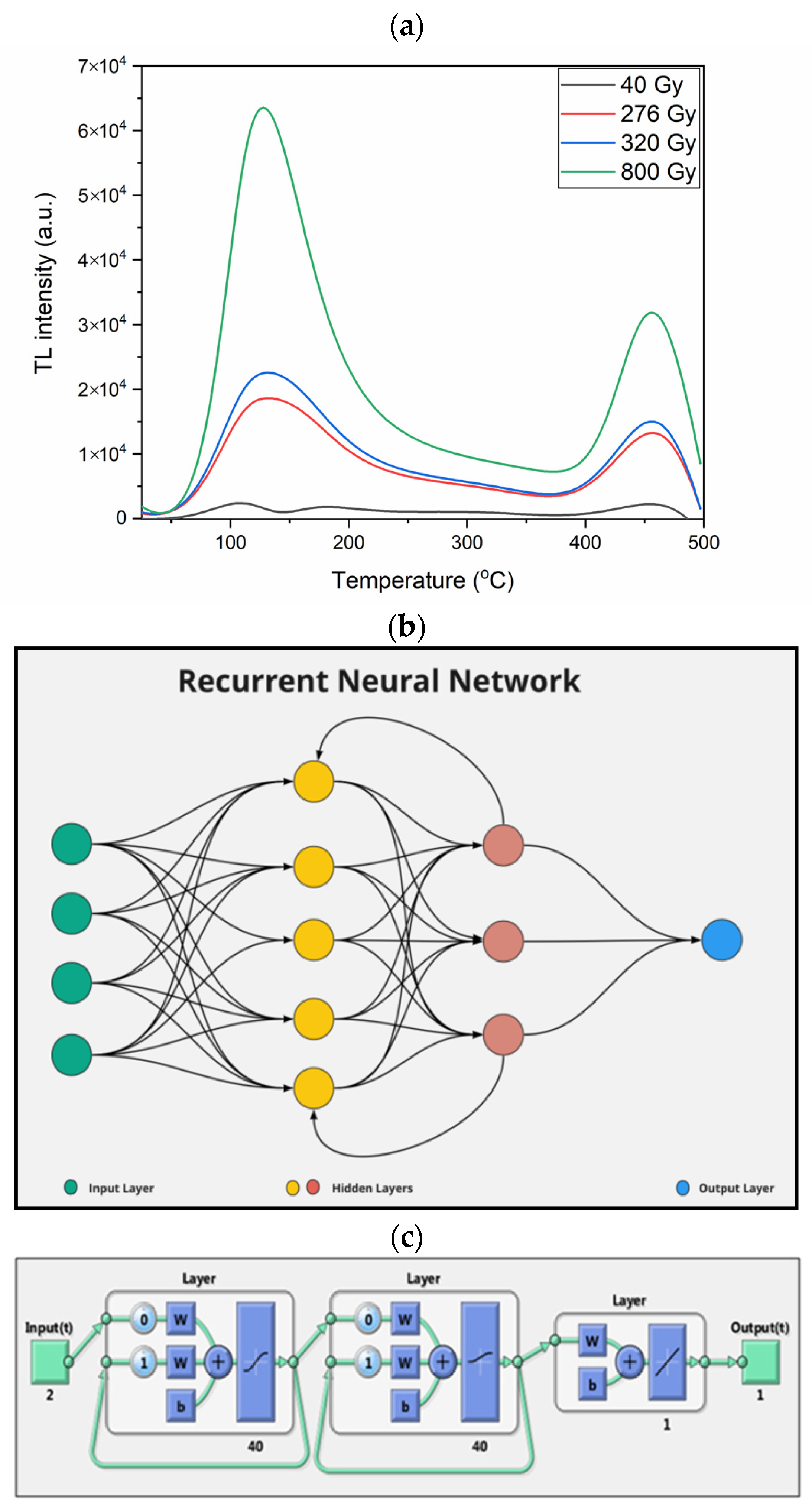
3.1. Materials
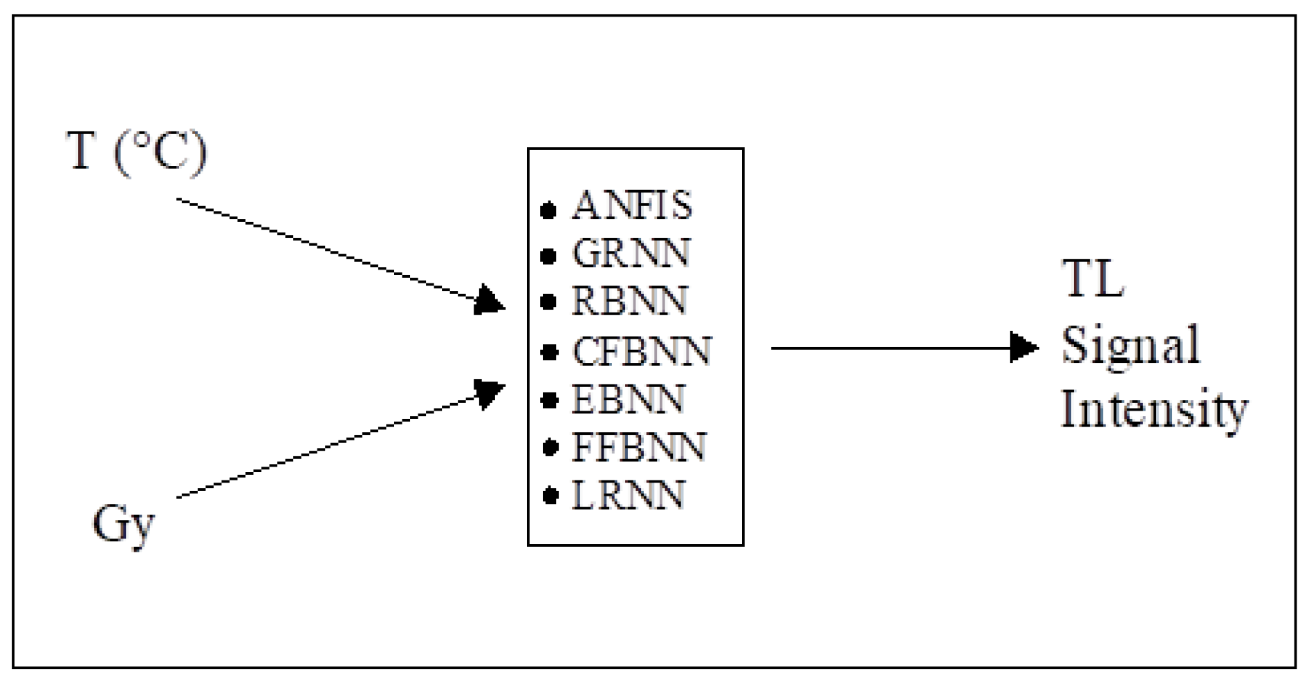
3.2. Methods
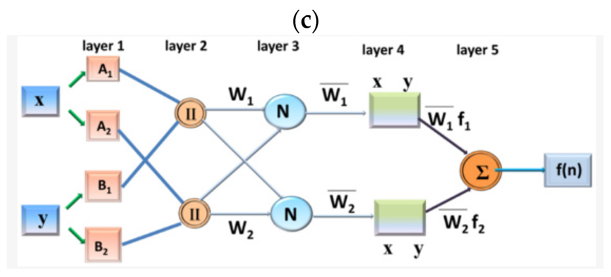
3.2.1. ANFIS
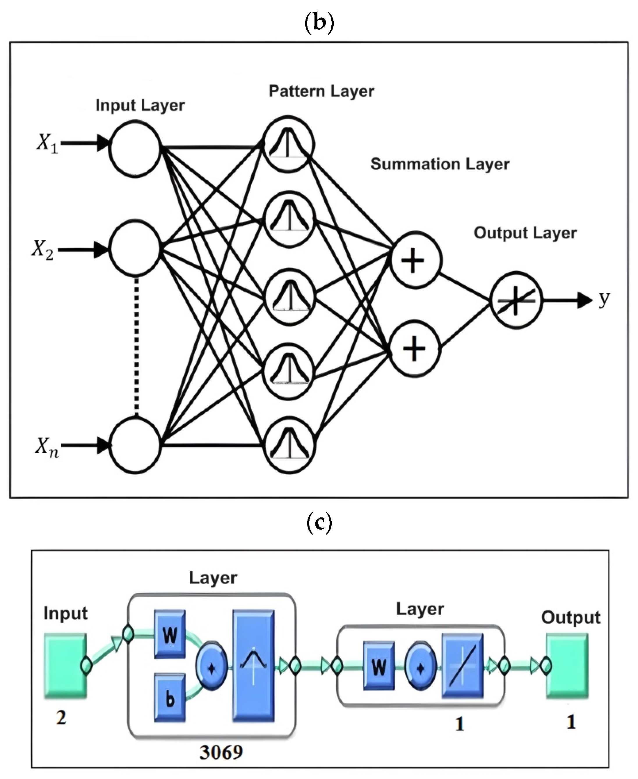
3.2.2. GRNN
3.2.3. RBNN
3.2.4. CFBNN
3.2.5. EBNN
3.2.6. FFBNN
3.2.7. LRNN
4. Results and Discussions
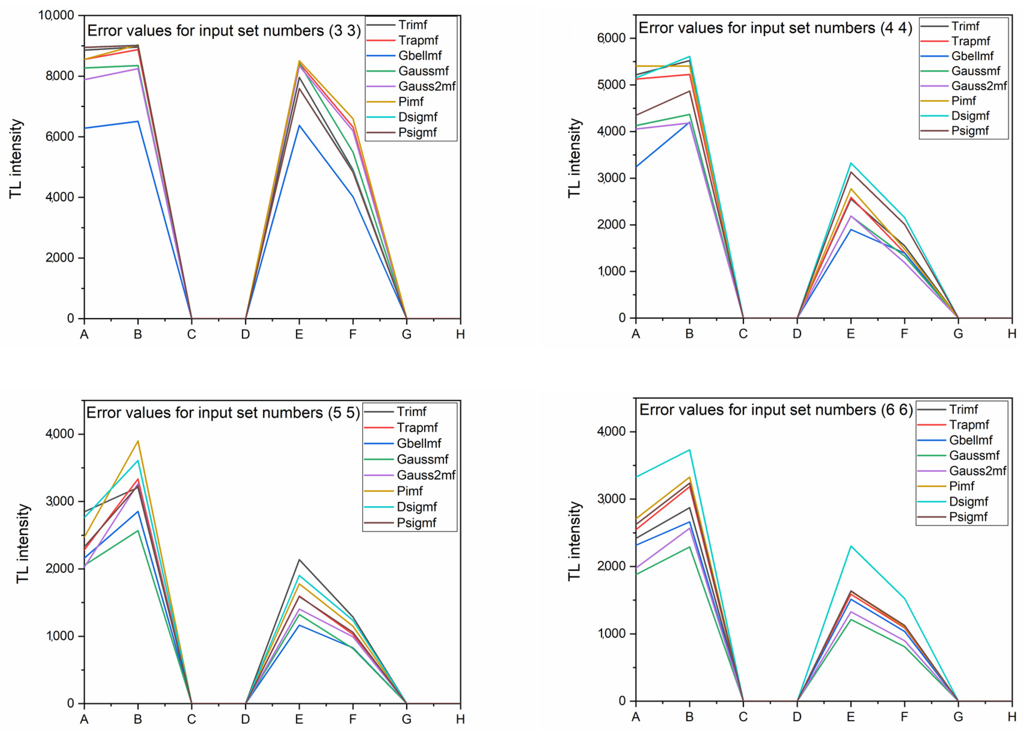
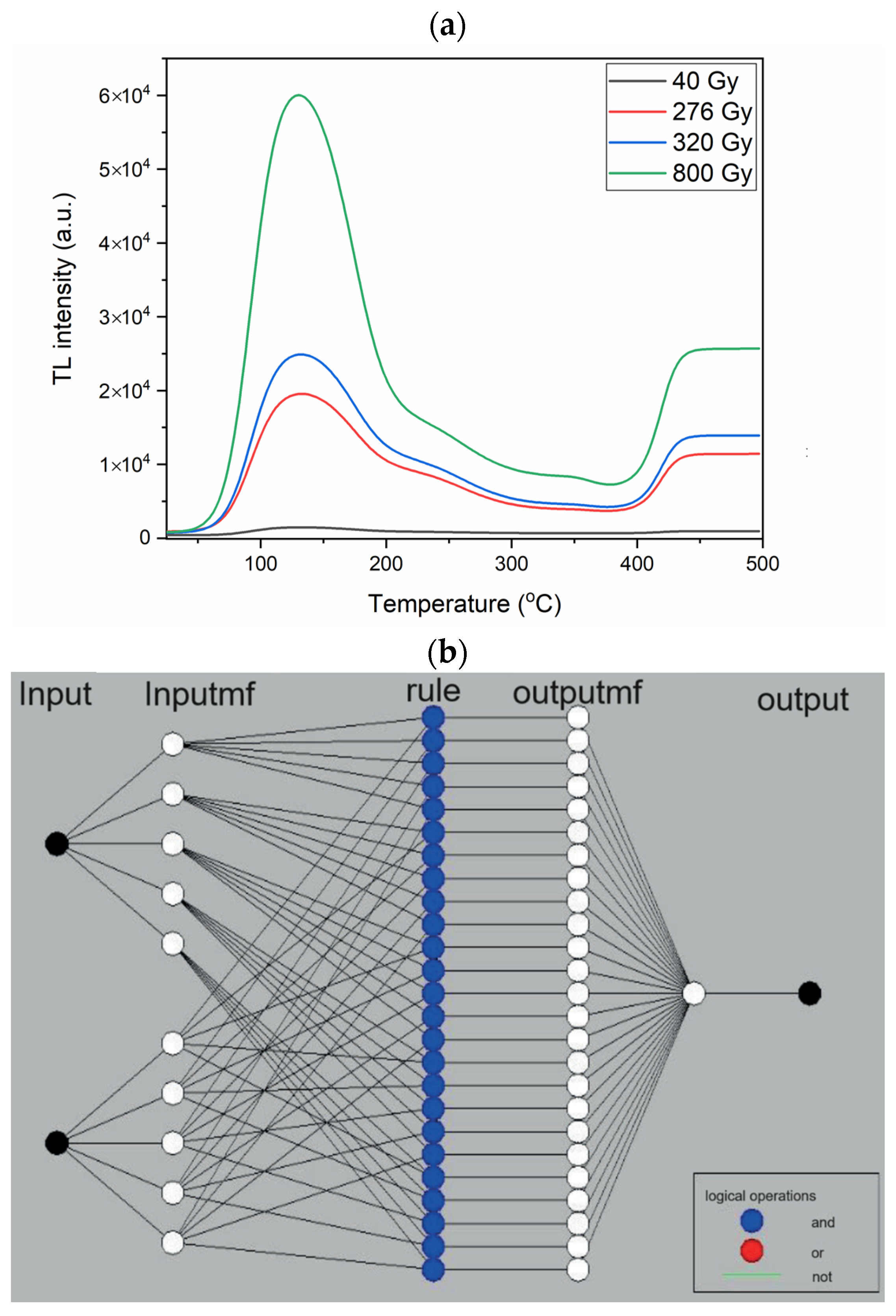
4.1. ANFIS
4.2. GRNN
4.3. RBNN
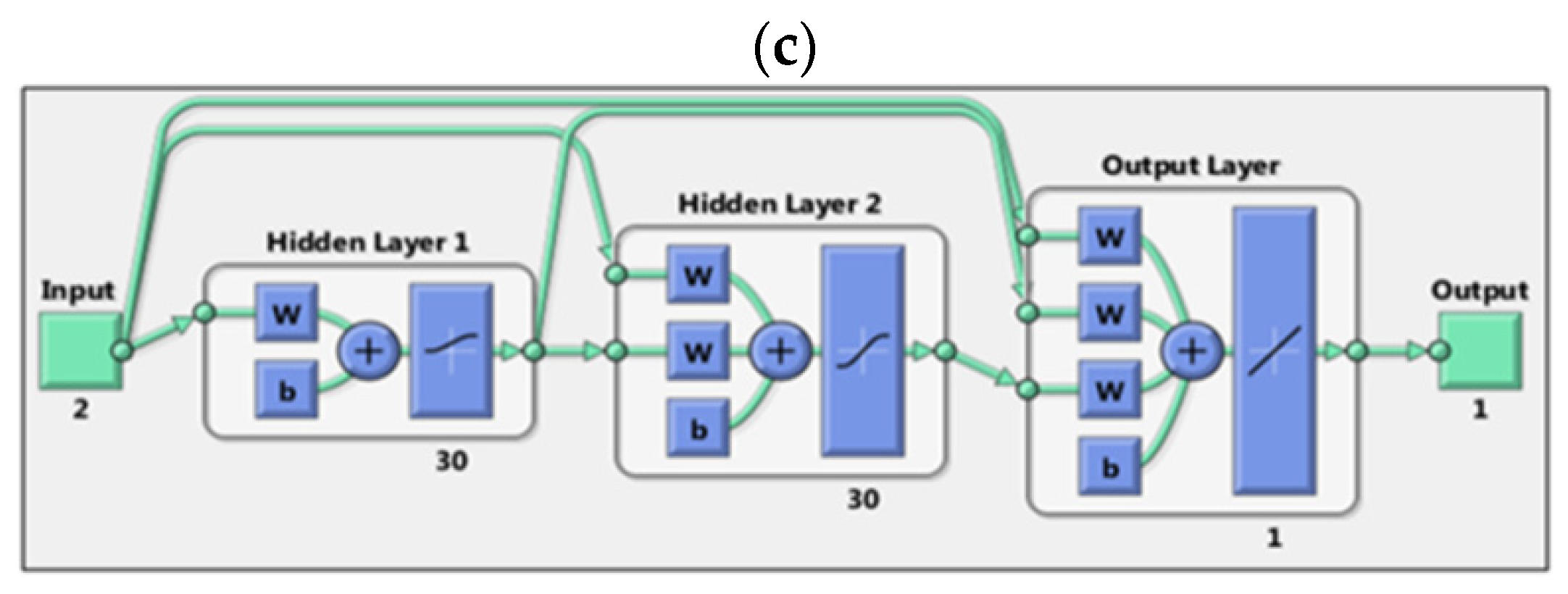
4.4. CFBNN
4.5. EBNN
4.6. FFBNN
4.7. LRNN
5. Conclusions
Funding
Institutional Review Board Statement
Informed Consent Statement
Data Availability Statement
Acknowledgments
Conflicts of Interest
References
- McKeever, S.W.S. Thermoluminescence of Solids; Cambridge University Press: Cambridge, UK, 1985. [Google Scholar]
- Aitken, M.J. Thermoluminescence Dating; Academic Press: London, UK, 1985. [Google Scholar]
- Dogan, T. Comparison of the thermoluminescence kinetic parameters for natural alkali-rich aluminosilicates minerals. Appl. Radiat. Isot. 2019, 149, 174–181. [Google Scholar] [CrossRef] [PubMed]
- Lyons, W.B.; Fitzpatrick, C.; Flanagan, C.; Lewis, E. A novel multipoint luminescent coated ultra violet fibre sensor utilising artificial neural network pattern recognition techniques. Sens. Actuators A Phys. 2004, 115, 267–272. [Google Scholar] [CrossRef]
- Karaman, Ö.A.; Ağır, T.T.; Arsel, İ. Estimation of solar radiation using modern methods. Alex. Eng. J. 2021, 60, 2447–2455. [Google Scholar] [CrossRef]
- Lee, S.Y.; Kim, B.H.; Lee, K.J. An application of artificial neural intelligence for personal dose assessment using a multi-area OSL dosimetry system. Radiat. Meas. 2001, 33, 293–304. [Google Scholar] [CrossRef] [PubMed]
- Kardan, M.R.; Koohi-Fayeghc, R.; Setayeshia, S.; Ghiassi-Neja, M. Fast neutron spectra determination by threshold activation detectors using neural networks. Radiat. Meas. 2004, 38, 185–191. [Google Scholar] [CrossRef]
- Nelson, M.S.; Rittenour, T.M. Using grain-size characteristics to model soil water content: Application to dose-rate calculation for luminescence dating. Radiat. Meas. 2015, 81, 142–149. [Google Scholar] [CrossRef]
- Yadollahi, A.; Nazemi, E.; Zolfaghari, A.; Ajorloo, A.M. Application of artificial neural network for predicting the optimal mixture of radiation shielding concrete. Prog. Nucl. Energy 2016, 89, 69–77. [Google Scholar] [CrossRef]
- Kröninger, K.; Mentzel, F.; Theinert, R.; Walbersloh, J. A machine learning approach to glow curve analysis. Radiat. Meas. 2019, 125, 34–39. [Google Scholar] [CrossRef]
- Işık, İ.; Işık, E.; Toktamış, H. Dose and fading time estimation of glass ceramic by using artificial neural network method. Dicle Üniversitesi Mühendislik Fakültesi Mühendislik Derg. 2021, 12, 47–52. [Google Scholar] [CrossRef]
- Derugin, E.; Kröninger, K.; Mentzel, F.; Nackenhorst, O.; Walbersloh, J.; Weingarten, J. Deep TL: Progress of a machine learning aided personal dose monitoring system. Radiat. Prot. Dosim. 2023, 199, 767–774. [Google Scholar] [CrossRef]
- Türkşen, İ.B. Dereceli (Bulanık) Sistem Modelleri; Abaküs Yayıncılık: İstanbul, Turkey, 2015. [Google Scholar]
- Baykal, N.; Beyan, T. Bulanık Mantık, Uzman Sistemler ve Denetleyiciler; Bıçaklar Kitabevi: Ankara, Turkey, 2004. [Google Scholar]
- Specht, D.F. A General Regression Neural Network. IEEE Trans. Neural Netw. 1991, 2, 568–576. [Google Scholar] [CrossRef] [PubMed]
- Sahroni, A. Brief Study of Identification System Using Regression Neural Network Based on Delay Tap Structures. GSTF J. Comp. 2013, 3, 17. [Google Scholar] [CrossRef]
- Sağıroğlu, Ş.; Beşdok, E.; Erler, M. Mühendislikte Yapay Zeka Uygulamaları I, Yapay Sinir Ağları; UFUK Yayıncılık: Kayseri, Turkey, 2003. [Google Scholar]
- Moody, J.; Darken, C.J. Fast Learning in Networks of Locally-Tuned Processing Units. Neural Comput. 1989, 1, 281–294. [Google Scholar] [CrossRef]
- Network Knowledge. Available online: https://www.mathworks.com/help/deeplearning/ref/cascadeforwardnet.html?s_tid=srchtitle_cascadeforwardnet_1 (accessed on 24 September 2021).
- Rumelhart, D.E.; Hinton, G.E.; Williams, R.J. Learning Representations by Back-Propagating Errors. Nature 1986, 323, 533–536. [Google Scholar] [CrossRef]
- Desai, V.S.; Crook, J.N.; Overstreet, G.A., Jr. A comparison of neural networks and linear scoring models in the credit union environment. Eur. J. Oper. Res. 1996, 95, 24–37. [Google Scholar] [CrossRef]
- Elman, J. Finding structure in time. Cogn. Sci. 1990, 14, 179–211. [Google Scholar] [CrossRef]
- Şen, Z. Yapay Sinir Ağları İlkeleri; Su Vakfı Yayınları: İstanbul, Turkey, 2004. [Google Scholar]
- Öztemel, E. Yapay Sinir Ağları, 3rd ed.; Papatya Yayıncılık: İstanbul, Turkey, 2012. [Google Scholar]
- Elmas, Ç. Yapay Zeka Uygulamaları, 3rd ed.; Seçkin Yayıncılık: Ankara, Turkey, 2016. [Google Scholar]
- Layer Recurrent Neural Network, Layrecnet Command. Available online: https://www.mathworks.com/help/deeplearning/ref/layrecnet.html?s_tid=srchtitle_layrecnet_1 (accessed on 26 September 2021).
- Design Layer Recurrent Neural Networks. Available online: https://www.mathworks.com/help/deeplearning/ug/design-layer-recurrent-neural-networks.html?searchHighlight=Design%20Layer-Recurrent%20Neural%20Networks&s_tid=srchtitle (accessed on 26 September 2021).
- Karunasingha, D.S.K. Root Mean Square Error or Mean Absolute Error? Use Their Ratio as Well. Inf. Sci. 2022, 585, 609–629. [Google Scholar] [CrossRef]
- Chicco, D.; Warrens, M.J.; Jurman, G. The Coefficient of Determination R-Squared is More Informative than SMAPE, MAE, MAPE, MSE and RMSE in Regression Analysis Evaluation. PeerJ Comput. Sci. 2021, 7, 623. [Google Scholar] [CrossRef]
- Schubert, A.L.; Hagemann, D.; Voss, A.; Bergmann, K. Evaluating the Model Fit of Diffusion Models with the Root Mean Square Error of Approximation. J. Math. Psychol. 2017, 77, 29–45. [Google Scholar] [CrossRef]
- de Myttenaere, A.; Golden, B.; Grand, B.L.; Rossi, F. Mean Absolute Percentage Error for Regression Models. Neurocomputing 2016, 192, 38–48. [Google Scholar] [CrossRef]
- Kucuk, N.; Kucuk, I. Computational modeling of thermoluminescence glow curves of zinc borate crystals. J. Inequal. Appl. 2013, 136, 136. [Google Scholar] [CrossRef]
- Isik, E.; Toktamis, D.; Er, M.B.; Hatib, M. Classification of thermoluminescence features of CaCO3 with long short-term memory model. Luminescence 2021, 36, 1684–1689. [Google Scholar] [CrossRef]
- Mentzel, F.; Derugin, E.; Jansen, H.; Kröninger, K.; Nackenhorst, O.; Walbersloh, J.; Weingarten, J. No More Glowingin the Dark: How Deep Learning Improves Exposure Date Estimation in Thermoluminescence Dosimetry. J. Radiol. Prot. 2020, 41, 4. [Google Scholar]
- Theinert, R.; Kröninger, K.; Lütfring, A.; Mender, S.; Mentzel, F.; Walbersloh, J. Fading Time and Irradiation Dose Estimation from Thermoluminescent Dosemeters Using Glow Curve Deconvolution. Radiat. Meas. 2018, 108, 20–25. [Google Scholar] [CrossRef]
- Toktamis, D.; Er, M.B.; Isik, E. Classification of thermoluminescence features of the natural halite with machine learning. Radiat. Eff. Defects Solids 2022, 177, 360–371. [Google Scholar] [CrossRef]
- Al-Mahasneh, A.J.; Anavatti, S.G.; Garratt, M.A. Review of Applications of Generalized Regression Neural Networks in Identif. and Control of Dynamic Systems. arXiv 2018, arXiv:1805.11236v1. [Google Scholar]


| Spread = 0.01 | Spread = 0.1 | Spread = 1 | Spread = 10 | Spread = 100 | |
|---|---|---|---|---|---|
| Training R2 | 1 | 1 | 0.9992 | 0.9975 | 0.5958 |
| Testing R2 | 0.9563 | 0.9563 | 0.9558 | 0.9547 | 0.5550 |
| Training RSE | 0 | 0 | 163.48 | 330.99 | 6645.55 |
| Testing RSE | 738.81 | 738.81 | 756.07 | 738.88 | 3897.21 |
| Training MAE | 0 | 0 | 0.0397 | 0.1828 | 2.1079 |
| Testing MAE | 0.2793 | 0.2793 | 0.2854 | 0.2668 | 1.4342 |
| sc: 0.01 eg: 1.10−11 | sc: 0.1 eg: 1.10−11 | sc: 0.1 eg: 0.1 | sc: 1 eg: 1 | sc: 10 eg: 10 | sc: 0.02 eg: 0.01 | |
|---|---|---|---|---|---|---|
| Training R2 | 1 | 1 | 1 | 0.9999 | 0.9999 | 1 |
| Testing R2 | 4.94 × 10⁻³⁰ | 4.94 × 10⁻³⁰ | 2.03 × 10⁻³¹ | 8.69 × 10⁻³¹ | 3.12 × 10⁻³² | 4.94 × 10⁻³⁰ |
| Training RSE | 1.37 × 10⁻⁹ | 1.37 × 10⁻⁹ | 2.8867 | 6.1533 | - | 1.37 × 10⁻⁹ |
| Testing RSE | 3349.34 | 3349.34 | 3348.67 | 3349.85 | 3339.81 | 3349.34 |
| Training MAE | 3.96 × 10⁻¹³ | 3.96 × 10⁻¹³ | 0.00027 | 0.00099 | 0.00452 | 3.96 × 10⁻¹³ |
| Testing MAE | 1 | 1 | 0.99906 | 1.00071 | 0.98652 | 1 |
| Network Type | Training Function | Layer 1 Transfer Function | Layer 1 Neuron | Layer 2 Transfer Function | Layer 2 Neuron | Layer 3 Transfer Function | Layer 3 Neuron | |
|---|---|---|---|---|---|---|---|---|
| 1 | Cas. For. Backp. | TRAINBFG | LOGSIG | 10 | PURELIN | 1 | - | - |
| 2 | Cas. For. Backp. | TRAINLM | TANSIG | 20 | PURELIN | 1 | - | - |
| 3 | Cas. For. Backp. | TRAINSCG | LOGSIG | 30 | TANSIG | 30 | PURELIN | 1 |
| 4 | Cas. For. Backp. | TRAINOSS | TANSIG | 40 | LOGSIG | 40 | PURELIN | 1 |
| Train. R | Valid. R | Test. R | All. R | MSE | Train R2 | Test. R2 | Train. RSE | Test. RSE | Train MAE | Test MAE | |
|---|---|---|---|---|---|---|---|---|---|---|---|
| 1 | 0.8921 | 0.8799 | 0.8409 | 0.8837 | 3.20 × 10⁷ | 0.78 | 0.70 | 5098.6 | 2817.27 | 2.33 | 1.33 |
| 2 | 0.9987 | 0.9982 | 0.9985 | 0.9986 | 4.84 × 10⁵ | 0.99 | 0.63 | 742.74 | 3611.56 | 0.39 | 0.96 |
| 3 | 0.9993 | 0.9988 | 0.9994 | 0.9992 | 3.08 × 10⁵ | 0.99 | 0.68 | 336.23 | 3000.46 | 0.19 | 0.71 |
| 4 | 0.9992 | 0.9991 | 0.9990 | 0.9991 | 2.28 × 10⁵ | 0.99 | 0.56 | 346.09 | 5051.94 | 0.20 | 1.73 |
| Network Type | Training Function | Layer 1 Transfer Function | Layer 1 Neuron | Layer 2 Transfer Function | Layer 2 Neuron | Layer 3 Transfer Function | Layer 3 Neuron | |
|---|---|---|---|---|---|---|---|---|
| 1 | Elman Backp. | TRAINBFG | LOGSIG | 10 | PURELIN | 1 | - | - |
| 2 | Elman Backp. | TRAINLM | TANSIG | 20 | PURELIN | 1 | - | - |
| 3 | Elman Backp. | TRAINSCG | LOGSIG | 30 | TANSIG | 30 | PURELIN | 1 |
| 4 | Elman Backp. | TRAINOSS | TANSIG | 40 | LOGSIG | 40 | PURELIN | 1 |
| Train. R | Valid. R | Test. R | All. R | MSE | Train R2 | Test. R2 | Train. RSE | Test. RSE | Train MAE | Test MAE | |
|---|---|---|---|---|---|---|---|---|---|---|---|
| 1 | - | - | - | - | 7.29 × 10⁷ | 0.45 | 0.40 | 7091.9 | 4304.59 | 2.10 | 1.67 |
| 2 | - | - | - | - | 3.08 × 10⁵ | 0.99 | 0.96 | 521.05 | 889.30 | 0.29 | 0.32 |
| 3 | - | - | - | - | 6.84 × 10⁶ | 0.95 | 0.93 | 1625.4 | 963.83 | 0.53 | 0.36 |
| 4 | - | - | - | - | 7.46 × 10⁵ | 0.99 | 0.98 | 635.54 | 440.95 | 0.28 | 0.16 |
| Network Type | Training Function | Layer 1 Transfer Function | Layer 1 Neuron | Layer 2 Transfer Function | Layer 2 Neuron | Layer 3 Transfer Function | Layer 3 Neuron | |
|---|---|---|---|---|---|---|---|---|
| 1 | Feed-For. Backp. | TRAINBFG | LOGSIG | 10 | PURELIN | 1 | - | - |
| 2 | Feed-For. Backp. | TRAINLM | TANSIG | 20 | PURELIN | 1 | - | - |
| 3 | Feed-For. Backp. | TRAINSCG | LOGSIG | 30 | TANSIG | 30 | PURELIN | 1 |
| 4 | Feed-For. Backp. | TRAINOSS | TANSIG | 40 | LOGSIG | 40 | PURELIN | 1 |
| Train. R | Valid. R | Test. R | All. R | MSE | Train R2 | Test. R2 | Train. RSE | Test. RSE | Train MAE | Test MAE | |
|---|---|---|---|---|---|---|---|---|---|---|---|
| 1 | 0.9581 | 0.9591 | 0.9412 | 0.9561 | 1.37 × 10⁷ | 0.91 | 0.90 | 2554.6 | 1220.40 | 1.15 | 0.57 |
| 2 | 0.9978 | 0.9968 | 0.9977 | 0.9976 | 8.37 × 10⁵ | 0.99 | 0.98 | 845.97 | 628.65 | 0.43 | 0.30 |
| 3 | 0.9992 | 0.9990 | 0.9990 | 0.9991 | 2.45 × 10⁵ | 0.99 | 0.72 | 314.62 | 2227.87 | 0.21 | 0.54 |
| 4 | 0.9992 | 0.9991 | 0.9984 | 0.9991 | 2.39 × 10⁵ | 0.99 | 0.82 | 366.35 | 1798.40 | 0.20 | 0.57 |
| Network Type | Training Function | Layer 1 Transfer Function | Layer 1 Neuron | Layer 2 Transfer Function | Layer 2 Neuron | Layer 3 Transfer Function | Layer 3 Neuron | |
|---|---|---|---|---|---|---|---|---|
| 1 | Layer Recurrent | TRAINBFG | LOGSIG | 10 | PURELIN | 1 | - | - |
| 2 | Layer Recurrent | TRAINLM | TANSIG | 20 | PURELIN | 1 | - | - |
| 3 | Layer Recurrent | TRAINSCG | LOGSIG | 30 | TANSIG | 30 | PURELIN | 1 |
| 4 | Layer Recurrent | TRAINOSS | TANSIG | 40 | LOGSIG | 40 | PURELIN | 1 |
| Train. R | Valid. R | Test. R | All. R | MSE | Train R2 | Test. R2 | Train. RSE | Test. RSE | Train MAE | Test MAE | |
|---|---|---|---|---|---|---|---|---|---|---|---|
| 1 | - | - | - | - | 7.96 × 10⁷ | 0.45 | 0.40 | 6575.9 | 3965.81 | 1.87 | 1.45 |
| 2 | - | - | - | - | 3.67 × 10⁵ | 0.99 | 0.72 | 507.67 | 2389.23 | 0.25 | 0.39 |
| 3 | - | - | - | - | 1.06 × 10⁶ | 0.99 | 0.98 | 762.05 | 476.37 | 0.35 | 0.19 |
| 4 | - | - | - | - | 8.47 × 10⁵ | 0.99 | 0.98 | 706.91 | 463.16 | 0.31 | 0.18 |
| Network Type | Train. 5% Error | Test. 5% Error | Train. 10% Error | Test. 10% Error | Train. 15% Error | Test. 15% Error | |
|---|---|---|---|---|---|---|---|
| 1 | EBNN | 37.30% | 32.70% | 58.35% | 62.18% | 80.80% | 87.95% |
| 2 | LRNN | 33.69% | 30.46% | 52.55% | 54.92% | 64.71% | 68.63% |
| 3 | FFBNN | 32.68% | 20.16% | 51.80% | 37.63% | 64.67% | 52.24% |
| 4 | GRNN | 97.97% | 13.53% | 97.97% | 24.46% | 97.97% | 36.11% |
| 5 | ANFIS | 26.09% | 27.95% | 45.12% | 49.64% | 57.57% | 64.24% |
| 6 | CFBNN | 61.51% | 14.06% | 73.15% | 23.92% | 79.96% | 33.33% |
| 7 | RBNN | 96.64% | 0 | 97.13% | 0 | 97.36% | 0 |
| Network Type | Train. R2 | Test. R2 | Train. RSE | Test. RSE | Train. MAE | Test. MAE | |
|---|---|---|---|---|---|---|---|
| 1 | EBNN | 0.99 | 0.98 | 635.54 | 440.95 | 0.28 | 0.16 |
| 2 | LRNN | 0.99 | 0.98 | 706.91 | 463.16 | 0.31 | 0.18 |
| 3 | FFBNN | 0.99 | 0.98 | 845.97 | 628.65 | 0.43 | 0.30 |
| 4 | GRNN | 1.00 | 0.95 | 0.00 | 738.81 | 0.00 | 0.27 |
| 5 | ANFIS | 0.97 | 0.96 | 1213.37 | 808.03 | 0.39 | 0.21 |
| 6 | CFBNN | 0.99 | 0.68 | 336.23 | 3000.46 | 0.19 | 0.71 |
| 7 | RBNN | 0.99 | 3.12 × 10⁻³² | - | 3339.81 | 0.004 | 0.98 |
Disclaimer/Publisher’s Note: The statements, opinions and data contained in all publications are solely those of the individual author(s) and contributor(s) and not of MDPI and/or the editor(s). MDPI and/or the editor(s) disclaim responsibility for any injury to people or property resulting from any ideas, methods, instructions or products referred to in the content. |
© 2023 by the author. Licensee MDPI, Basel, Switzerland. This article is an open access article distributed under the terms and conditions of the Creative Commons Attribution (CC BY) license (https://creativecommons.org/licenses/by/4.0/).
Share and Cite
Dogan, T. A Comparison of the Use of Artificial Intelligence Methods in the Estimation of Thermoluminescence Glow Curves. Appl. Sci. 2023, 13, 13027. https://doi.org/10.3390/app132413027
Dogan T. A Comparison of the Use of Artificial Intelligence Methods in the Estimation of Thermoluminescence Glow Curves. Applied Sciences. 2023; 13(24):13027. https://doi.org/10.3390/app132413027
Chicago/Turabian StyleDogan, Tamer. 2023. "A Comparison of the Use of Artificial Intelligence Methods in the Estimation of Thermoluminescence Glow Curves" Applied Sciences 13, no. 24: 13027. https://doi.org/10.3390/app132413027
APA StyleDogan, T. (2023). A Comparison of the Use of Artificial Intelligence Methods in the Estimation of Thermoluminescence Glow Curves. Applied Sciences, 13(24), 13027. https://doi.org/10.3390/app132413027