Numerical Analysis of Low-Cost Recognition of Tunnel Cracks with Compressive Sensing along the Railway

Abstract

Currently, the use of microseismic detection technology for crack detection and localization in rock masses has great potential in detecting structural damage. As engineering safety has always been a very important issue, this study investigated the problem of multi-crack identification in rock masses within the environment of track tunnels using transient waves. A tunnel rock was modeled using MIDAS GTS NX software (2019.v1.2) and a crack transient wave model in the frequency domain was obtained through data analysis and simulation. Then, this was combined with compressive sensing techniques to locate and detect multiple cracks in tunnel rock. The performance of the proposed approach was validated through experimental simulations, which included experiments on differences in the number of cracks, as well as spatial samples. The experimental results indicate that the technique performs well for single-crack localization in tunnel rock mass, where the average localization error is 4 m. Meanwhile, the localization error is larger in multi-crack localization, and the number of spatial sample points set using compressive sensing also has a large impact on the experimental results.

1. Introduction

In the field of track tunnel engineering, engineering safety holds exceptional significance. Strengthening the real-time monitoring of tunnel rock mass stress is a common practice in track tunnel construction to prevent accidents, such as tunnel collapse [1]. Currently, microseismic detection technology is widely used in tunnel disaster recognition and crack monitoring. When cracks appear in rock, they release strain energy and propagate elastic waves to the surroundings [2,3,4,5]. Crack detection based on visual and optical instrument assistance is currently the main means of daily inspection [6,7], but the method is time consuming and labor intensive, and the detection data carry a certain degree of subjectivity and are not sensitive to early cracks. There have been many research works on crack localization and identification; some of them have focused on the study of elastic wave propagation in a single medium [8,9], while others have analyzed the propagation and attenuation characteristics of R-waves in non-uniform media [10,11]. Most of them have focused on the study of propagation characteristics of elastic waves and few work on specific crack localization detection techniques.

In recent years, theoretical models for leak detection in pipelines in frequency-domain transient waves (pressure) have been studied [12]. Frequency-domain transient waves have great performance in terms of localization detection accuracy. In the research on crack identification, significant progress has been made in various aspects, including (1) analysis using the reverse transient method [13,14,15,16], (2) integration of transient damping techniques [17,18,19], (3) utilization of reflection techniques in the time domain [20,21,22], and (4) identification based on frequency-domain responses [23,24,25,26]. In this study, the aforementioned frequency-domain methods of transient waves were applied to crack localization and monitoring in tunnels. By conducting experimental simulations, the effect of localization detection can be simulated, which greatly simplifies the estimation problem of multiple cracks.

Despite the aforementioned work, there are still many unresolved issues in multi-crack identification. Solving the identification and localization problem of multiple cracks is challenging; the number of cracks in practical applications was previously unknown. Previous studies have mainly focused on identifying and locating individual cracks to simplify the process. As the number of cracks increases, the computational complexity grows rapidly. As a result, a new low-cost approach was needed to make the estimation process less sensitive to the number of cracks.

With the development of compressive sensing (CS) technology [27], it has been increasingly utilized in various fields. In simple terms, CS leverages the sparsity of signals in a domain to achieve accurate signal reconstruction at low sampling rates, thereby breaking the conventional Nyquist sampling criterion under specific conditions. Currently, CS is used successfully in image processing and communications [28,29,30,31,32,33]. In the context of crack detection in tunnel rock mass within the field of railway transportation, there has been limited work. Due to the spatial sparseness of the crack locations in the whole tunnel, the transient wave model for multi-crack identification can be linearly represented in terms of crack size but not in terms of crack location [26]. Nonetheless, the actual cracks within the tunnel can be considered sparse; therefore, investigating the problem of multi-crack localization using a sparse structure became a viable approach.

By establishing a transient wave model in the frequency domain for tunnel rock masses, using the geotechnical analysis software MIDAS GTS NX 2019v1.2, a transient wave model suitable for track tunnel rock masses was simulated and obtained the corresponding pressure transfer function through data analysis, which can reflect the propagation relationship.

This work was a CS-based multi-crack identification technique, due to the nonlinearity of the measurement model with respect to crack parameters, directly modeling and estimating the data, which obtained from real-world applications can be highly challenging. To address this issue, spatial sampling techniques were employed to transform the application problem into a defined space, thereby converting the problem of crack localization into a mathematical problem for modeling and solution.

Using MATLAB software (R2023a) with simulation analysis, the facilitation of further evaluation of the performance of this technique can be obtained. For a single-crack case, the average localization error is approximately 4 m. For the localization of two or more cracks, the experimental simulation results show that the average localization error is related to the distance between multiple cracks, and when the distance between multiple crack points is short, larger errors or missed detections will be caused.

2. Materials and Methods

The pressure-domain transient wave model for tunnel rock masses is elucidated and the presence of multiple cracks within the rock mass can be simulated. Based on this, the mathematical relationship between the tunnel cracks and the transmission of pressure-domain transient waves can be derived.

2.1. Transient Wave Model in the Frequency Domain of the Pressure of Tunnel Rock

Considering a tunnel rock mass with dimensions of 100 m in length, 50 m in width, and 50 m in height. Through simulation, modeling of the rock mass and setting its properties was based on real-world mechanical parameters. For illustration purposes, this model simulated a common rock mass with a density of 2730 kg/m³, an elastic modulus of 11 GPa, and a Poisson’s ratio of 0.21. The simulation was conducted using the Midas GTS NX (2019.v1.2) geotechnical analysis software. A grid system within the tunnel was created, with 50 observation points ($c_i$, where $\mathrm{i}=\mathrm{1,2},\dots ,50$) evenly distributed along the 100 m length of the rock mass. At one end of the rock mass, dynamic loads in the form of concentrated forces were applied. Table 1 lists some of the simulated data

Table 1. Position-dependent pressure data at specified angular frequency (200$\mathsf{\pi }$ as an example).

Angular Frequency	Measuring Point Coordinates (m)	Pressure Data (N)
628.3185	1	3.262333
628.3185	2	2.673342
628.3185	3	2.211276
628.3185	4	1.845488
628.3185	5	1.553216
628.3185	6	1.318036
628.3185	7	1.127432
628.3185	8	0.971705
628.3185	9	0.843691
628.3185	10	0.737694
…	...	…

Then, we performed experimental simulations, which consisted of two parts:

Simulating the perfect rock mass under dynamic loads of different angular frequencies to obtain the corresponding data ${\mathrm{Z}}^0({\mathrm{c}}_{\mathrm{i}};\mathsf{\omega })$; simulating the practical rock mass with cracks under dynamic loads of different angular frequencies to obtain the corresponding data $\mathrm{Z}(c_i;\omega )$.

During the process of experimental simulation, the model design was based on the geological properties of the tunnel rock mass and the experimental requirements. Figure 1 illustrates the application of dynamic loads at the position and direction indicated by the red arrow in the tunnel, with loads applied at different angular frequencies. Figure 2 demonstrates the introduction of cracks within the rock mass, where a spherical cavity is used to simulate the cracks, representing their location and volume as an indication of their size.

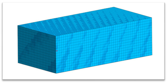
Figure 1. Dynamic load applied to a perfect rock mass in normal conditions.

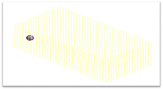
Figure 2. Dynamic load applied to a perfect rock mass with cracks.

2.2. Data Analysis and Derivation

Based on the pressure frequency-domain transient wave transmission function described in [26], we adopted this model to establish the transmission law of pressure within the rock mass. Reference [12] proposed a pressure function related to position and angular frequency within the tunnel:

$$h_m^0\left(\omega \right)=-Z\left(\omega \right)\sinh \left(\mu \left(\omega \right)s_m\right)q_U\left(\omega \right),$$

(1)

here, $q_U\left(\omega \right)$ represents the head oscillation, $Z\left(\omega \right)$ is the characteristic impedance, $\mu \left(\omega \right)$ is the propagation function, consisting of two constants with angular frequency as the independent variable, $s_m$ is the distance from the loading point to the rock mass, and $\omega$ is the angular frequency of the applied dynamic load. This function is position- and angular frequency-dependent, representing the theoretical pressure value in the absence of cracks at the distance $s_m$ from the loading point. The specific physical parameters of the formula are provided in Appendix A.

Normalizing the two sets of observations $Z^0(d_i;\omega )$ and $\mathrm{Z}(d_i;\omega )$. Normalization can provide several benefits, including: (1) accelerating convergence; (2) preventing bias in feature weighting; (3) improving model performance; and (4) enhancing interpretability.

Proposing an expression for the pressure frequency-domain transient wave model of the tunnel rock mass:

$$H_M^0\left(\omega \right)=-\left(\frac{a\sqrt{-{\omega }^2+ib\omega }}{ic\omega }\right)\sinh \left(\frac{\sqrt{-{\omega }^2+ib\omega }}{a}\ast s_m\right)\mathrm{d},$$

(2)

This expression is derived by simplifying Equation (1) and representing the constants as four unknown constants: a, b, c, and d. These four constants are the unknowns, which we aim to determine through experimental data. The observed data sets are used for machine learning training using the least squares method, with 20% of the data set used for testing.

By substituting the test set data into Equation (2) for solving, the four unknown constants a, b, c, and d are determined as 1.5724, 3.4860 × 10⁻⁶, 2.5129, and 9.2144 × 10⁻², respectively. Testing based on the training set achieved an MSE of 0.00197, indicating good accuracy of the pressure frequency-domain transient wave model for the tunnel rock mass.

Based on the simulated pressure frequency-domain transient wave model of the tunnel rock mass, along with the modeling of the rock mass, frequency-domain transient wave analysis can be performed, providing the transmission relationship of pressure frequency-domain transient waves with respect to position (as given by Equation (2)). This provides theoretical support for transforming the pressure difference vector into a vector representation of crack position and size.

3. Tunnel Rock System Model

A transient wave model was developed for locating and detecting cracks in the tunnel rock in a rail transit environment and a compressive sensing (CS) model for multi-crack detection problems was proposed.

Considering a rock mass (geotechnical properties are set as in Section 2, corresponding to common soft rock tunnels) with $N$ cracks, as shown in Figure 3, where setting the first and last ends to $s_U$ and $s_D$, setting ${\mathrm{x}}_n$ and ${\mathrm{v}}_n$ to be the position and size information of the $n$-th crack, $\forall n=1:N$, and assuming ${\mathrm{s}}_U<{\mathrm{x}}_1<{\mathrm{x}}_2\cdots <{\mathrm{x}}_N<{\mathrm{s}}_D$. A total of $M$ pressure sensors were deployed along the tunnel to collect observational results for crack identification, where $s_m$ denotes the location of the mth sensor installation, and the location is a section of the rock body that emits a dynamic load point.

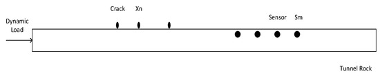
Figure 3. A tunnel rock mass with cracks and sensors.

Crack detection employing the frequency-domain transient wave model [12]. Based on the description in Section 2, it can be established that the pressure values, at the detection points, vary depending on the position and size of the cracks [26]. Thus, the pressure values can serve as the primary observations for determining the location and size of the cracks, which will be utilized in subsequent model development.

The data on pressure is collected by $M$ sensors for subsequent crack detection. $H_m\left(\omega \right)$ denotes the data collected by sensor $s_m$ at angular frequency $\omega$. The set of frequencies used in collecting data at $\mathsf{\Omega }$ has a total of $N_{\mathsf{\Omega }}$ angular frequencies

Setting the pressure values $\left\{H_m\left(\omega \right),\forall \omega \in \mathsf{\Omega }\right\}$ by sensor $s_m$, the pressure difference can be expressed as:

$$d_m\left(\omega \right)=H_m\left(\omega \right)-H_m^0\left(\omega \right),$$

(3)

where $H_m^0\left(\omega \right)$ is the theoretical pressure at $s_m$ when there are no cracks within the range $\left[0,{\mathrm{s}}_m\right]$, as given by Equation (2).

Expressing ${\mathrm{d}}_m\left(\omega \right)$ as a vector $\mathbf{d}\in {\mathbb{R}}^{N_{\mathsf{\Omega }}M}$:

$$\mathbf{d}=\mathrm{v}\mathrm{e}\mathrm{c}\left[d_m\left(\mathsf{\omega }\right)|\forall \mathsf{\omega }\in \mathsf{\Omega },\forall \mathrm{m}=1:\mathrm{M}\right],$$

(4)

here, setting $\mathbf{x}$ and $\mathbf{v}$ as the information about the location and size of the cracks in the tunnel, which can be obtained as:

$$\mathbf{x}=\mathrm{v}\mathrm{e}\mathrm{c}\left[{\mathrm{x}}_n|\forall \mathrm{n}=1:N\right],$$

(5)

$$\mathbf{v}=\mathrm{v}\mathrm{e}\mathrm{c}\left[{\mathrm{v}}_n|\forall \mathrm{n}=1:N\right],$$

(6)

where ${\mathrm{x}}_1<\cdots <{\mathrm{x}}_N$ for the position $\mathbf{x}$.

From the transient wave model derived in [12], a representation of the pressure difference of the crack related to the crack size and location information is written.

$$\mathbf{d}=\mathsf{\rho }\left(\mathbf{x}\right)\mathbf{v}+\mathsf{ϵ}.$$

(7)

This linearly represents the crack size but not the crack position. $\mathsf{ϵ}$ represents measurement errors, $\mathsf{\rho }\left(\mathbf{x}\right)\in {\mathbb{R}}^{N_{\mathsf{\Omega }}M\times N}$ is the measurement matrix, and the composition of the measurement matrix is related to the location information of the crack point, which can be expressed as:

$$\mathsf{\rho }\left(\mathbf{x}\right)=\left[\mathsf{\phi }\left(x_1\right),\dots ,\mathsf{\phi }\left(x_N\right)\right],$$

(8)

where $\mathsf{\phi }\left(x_N\right)$, $\mathrm{n}=1:N$, is the measurement function ${\psi }_m\left({\mathrm{x}}_n;\omega \right)$ dependent on the crack position ${\mathrm{x}}_n$, given by:

$$\mathit{\phi }\left({\mathrm{x}}_n\right)=\mathrm{vec}\left[{\psi }_m\left({\mathrm{x}}_n;\omega \right)\mid \forall \omega \in \mathsf{\Omega },\forall m=1:M\right],$$

(9)

and ${\psi }_m\left({\mathrm{x}}_n;\omega \right)$ is provided in [26], with the expression:

$${\psi }_m\left({\mathrm{x}}_n;\omega \right)=\left\{\begin{array}{c}\begin{array}{c}-\left(Z\right(\omega ){)}^2\sinh \left(\mu \left(\omega \right)\left({\mathrm{s}}_m-{\mathrm{x}}_n\right)\right)\sinh \left(\mu \left(\omega \right){\mathrm{x}}_n\right)q_U(\omega ),\hspace{0.25em}\hspace{0.25em}\hspace{0.25em}\hspace{0.25em}\mathrm{i}\mathrm{f}\hspace{0.25em}{\mathrm{x}}_n\le {\mathrm{s}}_m\\ 0,\hspace{0.25em}\hspace{0.25em}\hspace{0.25em}\hspace{0.25em}\hspace{0.25em}\hspace{0.25em}\hspace{0.25em}\hspace{0.25em}\hspace{0.25em}\hspace{0.25em}\hspace{0.25em}\hspace{0.25em}\hspace{0.25em}\hspace{0.25em}\hspace{0.25em}\hspace{0.25em}\hspace{0.25em}\hspace{0.25em}\hspace{0.25em}\hspace{0.25em}\hspace{0.25em}\hspace{0.25em}\hspace{0.25em}\hspace{0.25em}\hspace{0.25em}\hspace{0.25em}\hspace{0.25em}\hspace{0.25em}\hspace{0.25em}\hspace{0.25em}\hspace{0.25em}\hspace{0.25em}\hspace{0.25em}\hspace{0.25em}\hspace{0.25em}\hspace{0.25em}\hspace{0.25em}\hspace{1em}\hspace{1em}\hspace{1em}\hspace{1em}\hspace{1em}\hspace{1em}\hspace{0.25em}\hspace{0.25em}\hspace{0.25em}\mathrm{o}\mathrm{t}\mathrm{h}\mathrm{e}\mathrm{r}\mathrm{w}\mathrm{i}\mathrm{s}\mathrm{e}\end{array}\end{array}\right.$$

(10)

In Equation (9), the relevant unknown variables are represented in Equation (2). Based on the modeling analysis of the tunnel rock mass in this Section, the transient wave model in the tunnel rock mass allows for compressive sensing (CS) sparse modeling. This transforms the practical application problem into a mathematical problem for solution.

4. CS Sparse Model

In this Section, the process of transforming rock transient wave modeling to coefficient modeling is described, transforming the application problem into the problem of finding a sparse recovery signal.

4.1. Sparse Modeling of Pressure Differences

The purpose is to estimate the location and size of the crack based on the collected data $\mathbf{d}$. Directly estimating $\mathbf{x}$ and $\mathbf{v}$ is challenging due to the nonlinear relationship between $\mathbf{d}$ and $\mathbf{x}$ and $\mathbf{v}$. Proposing to use spatial sampling to transform a portion of the linear model into a sparse representation simplifies the associated signal processing. Consider $I$ spatial samples of crack positions $\mathit{\alpha }=\mathrm{v}\mathrm{e}\mathrm{c}\left[{\alpha }_i\mid \forall i=1:I\right]$, where ${\alpha }_i\in [s_U,s_D]$. These sample positions $\mathit{\alpha }$ represent potential crack positions.

The corresponding column vectors of the basis matrix of the spatial sample points ${\alpha }_i$ are:

$$\varphi \left({\alpha }_i\right)=\mathrm{vec}\left[{\psi }_m\left({\alpha }_i;\omega \right)\mid \forall \omega \in \mathsf{\Omega },\forall m=1:M\right],$$

(11)

where ${\psi }_m\left({\alpha }_i;\omega \right)$ depends on ${\alpha }_i$ and is given by Equation (8) with ${\alpha }_i$ substituted. Let $\mathbf{G}\left(\alpha \right)\in {\mathbb{R}}^{N_{\mathsf{\Omega }}M\times I}$ be the base matrix, defined as:

$$\mathbf{G}\left(\alpha \right)=\left[\varphi \left({\alpha }_1\right),\dots ,\varphi \left({\alpha }_I\right)\right],$$

(12)

where $N_{\mathsf{\Omega }}$ represents the number of frequencies utilized. Consequently, the measured value $\mathbf{d}$:

$$\mathbf{d}=\mathbf{G}\left(\alpha \right)\mathbf{t}+\mathsf{ϵ}+{\mathsf{ϵ}}_{\mathbf{s}},$$

(13)

The error ${\mathsf{ϵ}}_{\mathbf{s}}$ in this is due to the fact that the spatial sample points set during the spatial sample modeling cannot be aligned with the sensor sampling points. The vector $\mathbf{t}$ represents the sparse crack size signal, where its non-zero elements correspond to the actual crack sizes, and its support corresponds to the spatial samples closest to the actual crack positions. When setting up the spatial sample points, a larger number of spatial sample points are generally set up to obtain better results, so a small number of cracks in the tunnel rock mass can be regarded as sparse for the spatial sample point.

As shown in Figure 4, this illustrates the graphical representation of sparse modeling for crack detection in tunnel rock mass, where $\mathbf{d}=\mathbf{G}\left(\alpha \right)\mathbf{t}+\mathsf{ϵ}+{\mathsf{ϵ}}_{\mathbf{s}}$. From the figure, it can be observed that the measurement value $\mathbf{d}$ can be expressed as the product of $\mathbf{G}\left(\alpha \right)$ and the estimated value $\mathbf{t}$, where each column of $\mathbf{G}\left(\alpha \right)$ corresponds to $\varphi \left({\alpha }_i\right)$. The spatial sample points corresponding to the non-zero values in $\mathbf{t}$ represent possible crack locations in the rock mass, and the magnitude of the non-zero values represents the crack sizes.

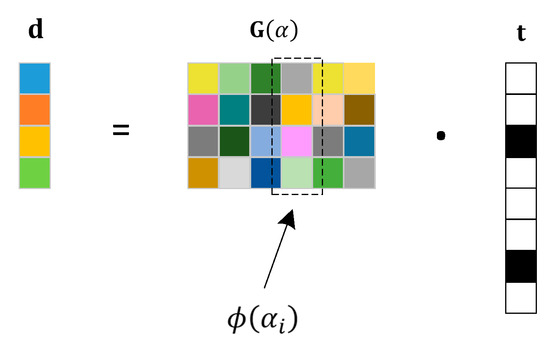
Figure 4. Sparse modeling explanation for crack detection.

4.2. Estimating Crack Positions $\mathit{x}$ and Sizes $\mathit{v}$

In the expression of Equation (12), by incorporating the known transient wave model, it is possible to represent the tunnel cracks by the recovered vector, which simultaneously provides information about the crack locations and sizes. Within the recovered vector, all non-zero entries correspond to crack points, with the position information reflected by the index of the entry, and the value at that position indicating the size of the respective crack; therefore, the focus is to estimate $\mathbf{t}$ from $\mathbf{d}$, translated into questions ${\rm P}0$.

$$\left({\rm P}0\right):$$

$$\widehat{\mathbf{t}}=arg\underset{\mathbf{t}}{\min }\left|\right|\mathbf{t}|{|}_0$$

$$\mathrm{s}.\mathrm{t}.\left|\right|\mathbf{d}-\mathbf{G}\left(\mathit{\alpha }\right)\mathbf{t}|{|}_2^2\le {\mathrm{d}}_{\mathrm{t}\mathrm{h}}$$

Here, $\left|\right|\mathbf{t}|{|}_0$ is the ${\mathcal{l}}_0$-norm, is the number of non-zero terms in the recovery vector, $\left|\right|\mathbf{d}-\mathbf{G}\left(\mathit{\alpha }\right)\mathbf{t}|{|}_2^2$ is the ${\mathcal{l}}_2$-norm, and ${\mathrm{d}}_{\mathrm{t}\mathrm{h}}$ is The set error threshold, ${\mathrm{d}}_{\mathrm{t}\mathrm{h}}=(1+{\varsigma }_{\mathrm{z}}){\sigma }^2$, where ${\varsigma }_{\mathrm{z}}\in \left[\mathrm{0.1,0.3}\right]$ and ${\sigma }^2$ is the variance of the measurement error $\mathsf{ϵ}$.

Problem ${\rm P}0$ is explained by the following lemma, where ${\mathcal{D}}_{(I,2)}=\left\{\mathit{\mu }\in {\mathbb{C}}^I:\parallel \mathit{\mu }{\parallel }_0\le 2\right\}$ represents the set of sparse signals:

Lemma 1. 

[The restricted isometry property (RIP) of $\mathit{G}\left(\mathit{\alpha }\right)$ for 2-sparse signals] The base matrix $\mathit{G}\left(\mathit{\alpha }\right)$ satisfies the following RIP for $\forall \mathit{\mu }\in {\mathcal{D}}_{(I,2)}$:

$$\left(1-{\delta }_{\left(2\right)}\right)\parallel \mathit{\mu }{\parallel }_2^2\le {∥C_{\left(2\right)}^{-1}\mathbf{G}\left(\mathit{\alpha }\right)\mathit{\mu }∥}_2^2\le \left(1+{\delta }_{\left(2\right)}\right)\parallel \mathit{\mu }{\parallel }_2^2,$$

(14)

the value of ${\delta }_{\left(2\right)}$ is defined as $({\lambda }_{max}-{\lambda }_{min})/({\lambda }_{max}+{\lambda }_{min})$, and $C_{\left(2\right)}$ is calculated as $({\lambda }_{max}+{\lambda }_{min})/2$, where ${\lambda }_{max}$ and ${\lambda }_{min}$ are obtained from Appendix B. The proof of Lemma 1 can be found in Appendix B.

Lemma 2. 

[For the error analysis of a single crack] There exists an optimal solution to the problem for a single crack based on a specific basis matrix $\mathit{G}\left(\mathit{\alpha }\right)$ under the transient wave model in the frequency domain, which has the following constraints:

$${∥{\mathbf{t}}^{\star }-\mathbf{t}∥}_2\le \frac{2\left(\parallel \mathit{ϵ}{\parallel }_2+{∥{\mathit{ϵ}}_s∥}_2\right)}{C_{\left(2\right)}\left(1-{\delta }_{\left(2\right)}\right)}$$

(15)

The proof of Lemma 2 is provided in Appendix C. The optimal solution to the problem ${\rm P}0$ is the one that is closest to the real signal with enough spatial sample points. By modeling the crack detection problem in tunnel rock mass using CS, the problem of crack detection is transformed into seeking the optimal solution of ${\rm P}0$.

5. Crack Detection Method Based on CS

In this Section, the logic of the sparse recovery algorithm and analysis of the algorithm are described. Then, based on the estimated value $\mathbf{d}$, the crack position $\mathbf{x}$ and crack size $\mathbf{v}$ are determined.

5.1. Reconstruction of Sparse Signals

Problem ${\rm P}0$ is a standard sparse recovery problem. For the selection of sparse recovery algorithms, the Orthogonal Matching Pursuit (OMP) algorithm is employed. According to Equation (12), given $\mathbf{G}\left(\mathit{\alpha }\right)$ and $\mathbf{d}$, the goal is to recover $\mathbf{t}$ from these values. It is evident that we need to fully utilize the sparsity of u. Based on the knowledge of linear algebra, $\mathbf{d}$ can be represented as a linear combination of the column vectors of matrix $\mathbf{G}\left(\mathit{\alpha }\right)$, where $\mathbf{t}$ acts as a weight for the column vectors of $\mathbf{G}\left(\mathit{\alpha }\right)$. As $\mathbf{t}$ is sparse, only a few column vectors in $\mathbf{G}\left(\mathit{\alpha }\right)$ significantly contribute to $\mathbf{d}$. The objective is to identify the column vectors that have a significant impact on $\mathbf{d}$. Simultaneously, based on the positions of the column vectors in $\mathbf{G}\left(\mathit{\alpha }\right)$, the positions of the non-zero elements in $\mathbf{t}$ can be determined. This is the fundamental application of the OMP algorithm in the crack estimation. Summarizing the pseudocode for the OMP algorithm to recover $\mathbf{t}$, the specific algorithm steps are as Algorithm 1 below:

Algorithm 1: The OMP-Based Sparse Signal Recovery

Input: Measurement values of pressure difference $\mathbf{d}$. Set algorithm parameters, such as $I$ and the setting of ${\mathrm{d}}_{\mathrm{t}\mathrm{h}}$ Initialize the index set $\mathcal{S}=\mathcal{\varnothing }$ and the set of spatial samples $\mathcal{A}=\{1,\dots ,I\}$ Set the measured value ${\mathbf{d}}_{\mathrm{♮}}=\mathbf{d}$ Loop through the following steps until ${∥{\mathbf{d}}_{\mathrm{♮}}∥}_2\le {\mathrm{d}}_{\mathrm{t}\mathrm{h}}$ Calculate ${\nu }_i=\frac{{\left(\varphi \left({\alpha }_{\mathit{i}}\right)\right)}^{\mathrm{H}}{\mathbf{d}}_{\mathrm{♮}}}{{∥\varphi \left({\alpha }_i\right)∥}_2},\forall i\in \mathcal{A}\setminus \mathcal{S}$ Find $i^{\star }$ such that $i^{\star }=arg\underset{i\in \mathcal{A}\setminus \mathcal{S}}{\max }\left|\right|{\nu }_i|{|}_2$ Gain the index set $\mathcal{S}$ as $\mathcal{S}=i^{\star }\cup \mathcal{S}$ Update the estimated value $\widehat{\mathbf{t}}$ as $\mathbf{t}=(\mathbf{G}\left(\mathit{\alpha }\right){)}^{†}\mathbf{d}$, where $(\mathbf{G}\left(\mathit{\alpha }\right){)}^{†}$ is the pseudo-inverse of $\mathbf{G}\left(\mathit{\alpha }\right)$ Calculation result of ${\mathbf{d}}_{\mathrm{♮}}=\mathbf{d}-\mathbf{G}\left({\mathit{\alpha }}_{\mathcal{S}}\right)\widehat{\mathbf{t}}$ Output: Estimated value $\widehat{\mathbf{t}}$

5.2. Determination of Crack Position and Size

Given $\widehat{\mathbf{t}}$, the crack position $\mathbf{x}$ and size $\mathbf{v}$ are determined. The computational steps used are to first set up an index set of spatial samples, expressed using the following Equation (14), which needs to be taken into account when setting up the index set, with respect to the previous values of the error thresholds:

$$\mathcal{K}\left(\widehat{\mathbf{t}};t_{\mathrm{t}\mathrm{h}}\right)=\left\{i\mid \mathfrak{R}\left\{{\widehat{\mathrm{t}}}_i\right\}\ge t_{\mathrm{t}\mathrm{h}},\forall i=1:I\right\},$$

(16)

$\mathfrak{R}\{•\}$ is used to represent the part of the real part of the complex number; subsequent problems on crack estimation are analyzed based on the part of the real part, and the estimate obtained by the specific algorithm can be expressed as follows:

$$\widehat{\mathbf{x}}=\mathrm{v}\mathrm{e}\mathrm{c}\left[x_i|\forall i\in \mathcal{K}\left(\widehat{\mathbf{t}};t_{\mathrm{t}\mathrm{h}}\right)\right];$$

(17)

$$\widehat{\mathbf{v}}=\mathrm{v}\mathrm{e}\mathrm{c}\left[\mathfrak{R}\left\{{\widehat{\mathrm{t}}}_i\right\}|\forall i\in \mathcal{K}\left(\widehat{\mathbf{t}};t_{\mathrm{t}\mathrm{h}}\right)\right],$$

(18)

${\widehat{\mathrm{t}}}_i$ represents the $i$th estimated value of $\widehat{\mathbf{t}}$.

Due to the error in the measurement estimation, there will be a projection of the error in the OMP basis matrix. So when setting the threshold $t_{\mathrm{t}\mathrm{h}}$, the value should be set to be larger than this projection of the error, but should not be too large in order to produce false detections and missed detections in the test. If $t_{\mathrm{t}\mathrm{h}}$ is set too large, it may lead to missed detections where small cracks may go undetected. On the other hand, if $t_{\mathrm{t}\mathrm{h}}$ is too small, it may cause false detections.

The recovery vector calculated using the algorithm is able to reflect the real crack situation to a certain extent; specifically, the estimated vector can be correlated with the real crack sparse signal throughout the transformation. For the algorithm, the signal with good recovery effect, it corresponds to the non-zero spatial sample point, which is actually very close to the real crack. This is also related to the setting of the algorithm parameter, as well as the setting of the spatial sample point; its $i$th element $t_{\mathrm{t}\mathrm{h}}$ will be equal to ${\mathrm{v}}_n$, otherwise it will be zero for $\forall i\in \mathcal{S}$. The OMP algorithm essentially comes up with a search for column vectors on $\mathbf{G}\left({\mathit{\alpha }}_{\mathcal{S}}\right)$ that contribute more to the measurements, while at the same time, based on the position of the column vectors in $\mathbf{G}\left({\mathit{\alpha }}_{\mathcal{S}}\right)$, the position of the non-zero elements in $\mathbf{t}$ can be determined.

6. Simulation Results

Simulating the leakage detection method based on compressive sensing (CS) to validate the experimental performance of the proposed scheme.

6.1. Simulation Setup

Considering the overall properties of the tunnel rock mass, a rectangular model with a length of 100 m and both width and height of 50 m was constructed. A scenario that involves a maximum of two cracks was built, with crack sizes ranging from $5\times {10}^{-4}{\mathrm{m}}^2$ to $10\times {10}^{-4}{\mathrm{m}}^2$. For this purpose, we adopted that $I=1000$ uniformly distributed spatial samples, and equally spaced $M=50$ sensors along the 100 m length of the tunnel rock mass for data acquisition. The frequency set $\mathsf{\Omega }$ was defined as $\mathsf{\Omega }=\left\{i\omega \right|\forall i=1:N_{\mathsf{\Omega }}\}$, where $N_{\mathsf{\Omega }}$ = 20.

The transmission relationship of frequency-domain transient waves in tunnel rock mass is explained in Section 2 of this study, based on the same material properties and relevant parameters, with the transfer function given by Equation (2).

6.2. Analysis of the Crack Detection Results of the OMP Algorithm

Analyzing the results of the experimental simulation in terms of a single crack as ll as two cracks.

6.2.1. Analysis of the Results for a Single Crack

The localization of individual cracks was simulated and analyzed. The simulated estimation of the leak location is shown in Figure 5, where the number of spatial sample points determines the localization accuracy. The average error in crack location analysis for a single crack was 4.3547 m. The method was not applied in tunnel crack detection, and a comparison of the average errors in [12] shows that the simulation error is decreased, and the cumulative distribution functions (CDFs) of the estimated crack position errors are shown in Figure 6.

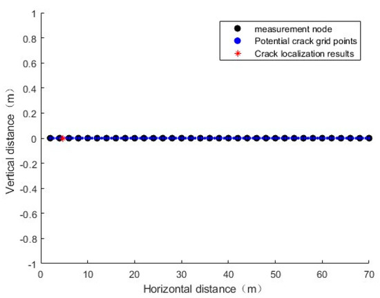
Figure 5. Monitoring results for a single crack.

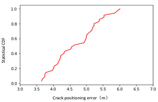
Figure 6. CDF of estimated error in single-crack position.

As shown in Figure 5, the simulation results obtained using the CS-based Orthogonal Matching Pursuit (OMP) algorithm are presented. The widely spaced points in the figure represent the measurement nodes, which are the locations where the sensor detection data are obtained. The closely spaced nodes represent the spatial sample points, which correspond to the potential crack locations.

As shown in Figure 6, the CDF of the error obtained from experimental simulation for a single crack indicates the distribution of the error. The error, denoted as $|\widehat{\mathrm{x}}-\mathrm{x}|$, represents the distance between the estimated position and the actual location of the crack, reflecting the accuracy of the estimation.

6.2.2. Analysis of Results for Two Cracks

The simulated estimation of crack positions for two cracks is shown in Figure 7. It can be observed that when the distance between the two cracks is close, the localization error increases. This indicates that the resolution for the performance of crack identification is degraded, which may be related to the wavelength of the transient wave, i.e., it is difficult to identify two cracks if the distance between them is smaller than the wavelength of the transient wave. The cumulative distribution functions (CDFs) of the estimated crack position errors are shown in Figure 8.

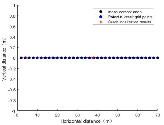
Figure 7. Monitoring results for two cracks.

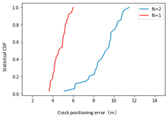
Figure 8. Cumulative distribution function of estimated error in two crack positions.

As shown in Figure 8, the CDF analysis of the error using the CS-based OMP algorithm for two cracks reveals that the detection error for two cracks is obviously greater than that for a single crack. During the simulation process, the distance between the two crack points has a significant impact on the error. The closer the crack points are, the larger the error will be, and it may even fail to detect the two cracks.

6.2.3. Analysis of Results for Different Spatial Sample Sizes (I)

Then, the performance of CS-based crack detection with different spatial sample sizes was analyzed. The range of values for the spatial sample number I is from 100 to 3000. The resulting crack position and size estimation errors relative to I are shown in Figure 9. The simulation results demonstrate that the crack detection performance improves as the number of spatial samples increases.

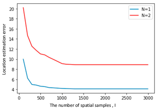
Figure 9. Relationship between crack detection error and spatial sample size.

The detection error for multiple cracks is greater than that for a single crack. The chosen spatial sample size I also has a substantial impact on the simulation results, as increasing the number of spatial samples can improve the accuracy of localization detection simulation to some extent.

7. Discussion and Conclusions

A compression-aware tunnel crack localization technique using the OMP recovery algorithm in the field of railway transportation is proposed. This CS-based crack detection method relies on the pressure difference at a point in the rock mass, considering both the presence and absence of cracks. As the linear representation of crack positions is not feasible, CS for modeling analysis, utilizing the OMP algorithm for signal recovery, is employed, followed by experimental simulations to analyze the results. The specific conclusions are as follows:

• The existing frequency-domain transient wave analysis method is applicable to tunnel rock mass environments. Through data analysis and simulation, the existing frequency-domain transient wave model is applied to the rail transportation field to solve the crack detection technology of tunnel rock, which has scalability.
• According to the proposed crack detection method, a more efficient scheme can be proposed for sensor deployment based on the results obtained from the simulations. Sensor placement in practical engineering can be guided by the expected error range, providing practical guidance for engineering applications.
• The accuracy of CS-based crack detection primarily depends on the number of spatial samples. These simulation results demonstrate that increasing the number of spatial sample points can reduce the error.
• The resolution of the proposed crack identification technique is related to the wavelength of the transient wave. If the distance between the two cracks is smaller than the wavelength of the transient wave, it becomes challenging to distinguish between the two crack points.
• In the experimental simulations for localization detection, the employed physical formulas and corresponding relationships are currently based on theoretical derivations. To improve the accuracy of localization, further research should focus on enhancing the content related to these aspects.

The CS-based framework utilizing the transient wave model shows potential for crack detection in tunnel rock masses. The findings of this study provide insights into the application of CS-based methods; different models should be used to study specific rock properties and future works will analyze the theoretical performance of CS-based tunnel crack detection.

References

- Callari, C. Coupled numerical analysis of strain localization induced by shallow tunnels in saturated soils. Comput. Geotech. 2004, 31, 193–207. [Google Scholar] [CrossRef]
- Li, Q.; Ling, F.; Hu, Q. Analysis of phased attenuation characteristics of elastic wave in coal measure strata. J. China Univ. Min. Technol. 2023, 52, 466–477. [Google Scholar]
- Li, Q.; Wu, X.; Zhai, C.; Hu, Q.; Ni, G.; Yan, F.; Xu, J.; Zhang, Y. Effect of frequency and flow rate of pulsating hydraulic fracturing on crack evolution. J. China Univ. Min. Technol. 2021, 50, 1067–1076. [Google Scholar]
- Zou, Y.; Wen, G.; Hu, Q. Theory analysis and experimental study of the spread and attenuation of acoustic emission in rock body. J. China Coal Soc. 2004, 29, 663–667. [Google Scholar]
- Yao, Q.; Wang, W.; Li, X. Study of mechanical properties and acoustic emission characteristics of coal measures under water-rock interaction. J. China Coal Soc. 2021, 50, 558–569. [Google Scholar]
- Worley, R.; Dewoolkar, M.M.; Xia, T.; Farrell, R.; Orfeo, D.; Burns, D.; Huston, D.R. Acoustic Emission Sensing for Crack Monitoring in Prefabricated and Prestressed Reinforced Concrete Bridge Girders. J. Bridge Eng. 2019, 24, 100–116. [Google Scholar] [CrossRef]
- Sieńko, R.; Zych, M.; Bednarski, Ł.; Howiacki, T. Strain and crack analysis within concrete members using distributed fibre optic sensors. Struct. Health Monit. 2019, 18, 1510–1526. [Google Scholar] [CrossRef]
- Guo, L.; Dai, F.; Xu, N. Research on MSFM-based microseismic source location of rock mass with complex velocities. Chin. J. Rock Mech. Eng. 2017, 36, 394–406. [Google Scholar]
- Chen, H.Z. Estimating elastic properties and attenuation factor from different frequency components of observed seismic data. Geophys. J. Int. 2019, 220, 794–805. [Google Scholar] [CrossRef]
- Chen, H.Z. Seismic frequency component inversion for elastic parameters and maximum inverse quality factor driven by attenuating rock physics models. Surv. Geophys. 2020, 41, 835–857. [Google Scholar] [CrossRef]
- Zhou, F.; Liu, H. Propagation characteristics of Rayleigh waves in unsaturated soils. Rock Soil Mech. 2019, 40, 3218–3226. [Google Scholar]
- Zhou, B.; Liu, A.; Wang, X.; She, Y.; Lau, V. Compressive Sensing-Based Multiple-Leak Identification for Smart Water Supply Systems. IEEE Internet Things J. 2018, 5, 1228–1241. [Google Scholar] [CrossRef]
- Liggett, J.A.; Chen, L.-C. Inverse transient analysis in pipe networks. J. Hydraul. Eng. 1994, 120, 934–955. [Google Scholar] [CrossRef]
- Nash, G.A.; Karney, B.W. Efficient inverse transient analysis in series pipe systems. J. Hydraul. Eng. 1999, 125, 761–764. [Google Scholar] [CrossRef]
- Vitkovsky, J.P.; Simpson, A.R.; Lambert, M.F. Leak detection and calibration using transients and genetic algorithms. J. Water Resour. Plan. Manag. 2000, 126, 262–265. [Google Scholar] [CrossRef]
- Covas, D.; Ramos, H. Case studies of leak detection and location in water pipe systems by inverse transient analysis. J. Water Resour. Plan. Manag. 2010, 136, 248–257. [Google Scholar] [CrossRef]
- Wang, X.-J.; Lambert, M.F.; Simpson, A.R.; Liggett, J.A.; Vitkovsky, J.P. Leak detection in pipelines using the damping of fluid transients. J. Hydraul. Eng. 2002, 128, 697–711. [Google Scholar] [CrossRef]
- Nixon, W.; Ghidaoui, M.S.; Kolyshkin, A.A. Range of validity of the transient damping leakage detection method. J. Hydraul. Eng. 2006, 132, 944–957. [Google Scholar] [CrossRef]
- Brunone, B. Transient test-based technique for leak detection in outfall pipes. J. Water Resour. Plan. Manag. 1999, 125, 302–306. [Google Scholar] [CrossRef]
- Covas, D.; Ramos, H.; Graham, N.; Maksimovic, C. Application of hydraulic transients for leak detection in water supply systems. Water Sci. Technol. Water Supply 2005, 4, 365–374. [Google Scholar] [CrossRef]
- Liou, J.C. Pipeline leak detection by impulse response extraction. J. Fluids Eng. 1998, 120, 833–838. [Google Scholar] [CrossRef]
- Mpesha, W.; Gassman, S.L.; Chaudhry, M.H. Leak detection in pipes by frequency response method. J. Hydraul. Eng. 2001, 127, 134–147. [Google Scholar] [CrossRef]
- Ferrante, M.; Brunone, B. Pipe system diagnosis and leak detection by unsteady-state tests. 1. Harmonic analysis. Adv. Water Resour. 2003, 26, 95–105. [Google Scholar] [CrossRef]
- Covas, D.; Ramos, H.; De Almeida, A.B. Standing wave difference method for leak detection in pipeline systems. J. Hydraul. Eng. 2005, 131, 1106–1116. [Google Scholar] [CrossRef]
- Lee, P.J.; Vítkovský, J.P.; Lambert, M.F.; Simpson, A.R.; Liggett, J.A. Frequency domain analysis for detecting pipeline leaks. J. Hydraul. Eng. 2005, 131, 596–604. [Google Scholar] [CrossRef]
- Wang, X.; Ghidaoui, M.S. Identification of multiple leaks in pipeline: Linearized model, maximum likelihood, and super-resolution localization. Mech. Syst. Signal Process. 2018, 107, 529–548. [Google Scholar] [CrossRef]
- Donoho, D.L. Compressed sensing. IEEE Trans. Inf. Theory 2006, 52, 1289–1306. [Google Scholar] [CrossRef]
- Oliveri, G.; Salucci, M.; Anselmi, N.; Massa, A. Compressive Sensing as Applied to Inverse Problems for Imaging: Theory, applications, current trends and open challenges. IEEE Antennas Propag. Mag. 2017, 59, 34–46. [Google Scholar] [CrossRef]
- Candes, E.J.; Wakin, M.B. An Introduction To Compressive Sampling. IEEE Signal Process. Mag. 2008, 25, 21–30. [Google Scholar] [CrossRef]
- Chen, J.; Gao, Y.; Ma, C.; Kuo, Y. Compressive sensing image re- construction based on multiple regulation constraints. Circuits Syst. Signal Process. 2017, 36, 1621–1638. [Google Scholar] [CrossRef]
- Wu, J.; Liu, F.; Jiao, L.C.; Wang, X. Compressive Sensing SAR Image Reconstruction Based on Bayesian Framework and Evolutionary Computation. IEEE Trans. Process. 2011, 20, 1904–1911. [Google Scholar] [CrossRef]
- Paredes, J.L.; Arce, G.R.; Wang, Z. Ultra-Wideband Compressed Sensing: Channel Estimation. IEEE J. Sel. Top. Signal Process. 2007, 1, 383–395. [Google Scholar] [CrossRef]
- Wylie, E.B.; Streeter, V.L.; Suo, L. Fluid Transients in Systems, Englewood Cliffs; Prentice Hall: Hoboken, NJ, USA, 1993; Volume 1, p. 464. [Google Scholar]
- Chaudhry, M.H. Applied Hydraulic Transients; Van Nostrand Reinhold: New York, NY, USA, 1979. [Google Scholar]
- Baraniuk, R.; Davenport, M.; DeVore, R.; Wakin, M. A simple proof of the restricted isometry property for random ma-trices. Constr. Approx. 2008, 28, 253–263. [Google Scholar] [CrossRef]
- Candes, E.J. The restricted isometry property and its implications for compressed sensing. Comptes Rendus Math. 2008, 346, 589–592. [Google Scholar] [CrossRef]
Disclaimer/Publisher’s Note: The statements, opinions and data contained in all publications are solely those of the individual author(s) and contributor(s) and not of MDPI and/or the editor(s). MDPI and/or the editor(s) disclaim responsibility for any injury to people or property resulting from any ideas, methods, instructions or products referred to in the content. |
© 2023 by the authors. Licensee MDPI, Basel, Switzerland. This article is an open access article distributed under the terms and conditions of the Creative Commons Attribution (CC BY) license (https://creativecommons.org/licenses/by/4.0/).