Robust Frontal Vehicle Pose Estimation Based on Structural Parameter Optimization Using Reliable Edge Point Sequences

Abstract

In order to enhance the stability of vehicle pose estimation within driving videos, a novel methodology for optimizing vehicle structural parameters is introduced. This approach hinges on evaluating the reliability of edge point sequences. Firstly, a multi−task and iterative convolutional neural network (MI−CNN) is constructed, enabling the simultaneous execution of four critical tasks: vehicle detection, yaw angle prediction, edge point location, and visibility assessment. Secondly, an imperative aspect of the methodology involves establishing a local tracking search area. This region is determined by modeling the limitations of vehicle displacement between successive frames. Vehicles are matched using a maximization approach that leverages point similarity. Finally, a reliable edge point sequence plays a pivotal role in resolving structural parameters robustly. The Gaussian mixture distribution of vehicle distance change ratios, derived from two measurement models, is employed to ascertain the reliability of the edge point sequence. The experimental results showed that the mean Average Precision (mAP) achieved by the MI−CNN network stands at 89.9%. A noteworthy observation is that the proportion of estimated parameters whose errors fall below the threshold of 0.8 m consistently surpasses the 85% mark. When the error threshold is set at less than 0.12 m, the proportion of estimated parameters meeting this criterion consistently exceeds 90%. Therefore, the proposed method has better application status and estimation precision.

1. Introduction

With the continuous development of autonomous driving technology and the wide application of robot navigation systems, vehicle pose estimation has emerged as a prominent research area in the realms of computer vision and machine perception. The objective of pose estimation is to precisely ascertain the position and orientation of a vehicle or robot within a three−dimensional space. This capability is paramount for achieving tasks such as autonomous navigation, environmental sensing, and safe driving. Vehicle pose estimation holds significant importance across a range of applications, although it has received comparatively less attention compared to human pose estimation. Recent technological advancements in the automotive industry have heightened the demand for precise vehicle pose estimation. This surge in interest is attributed to its applications in autonomous driving, traffic regulation, and scenario analysis. Vehicle pose estimation entails the identification of specific key points on a given vehicle. This task presents challenges due to the diverse array of vehicles characterized by variations in color, shape, and size.

Unlike human pose estimation, which is challenging due to the high degree of freedom of human joints and substantial occlusion, vehicle pose involves a more rigid structure with diverse types of occlusions. The expansion of the automotive industry has resulted in significant variability within each vehicle class, posing challenges in developing a robust method applicable to different types of vehicles. Moreover, camera viewpoints exhibit considerable variability in terms of vehicle height. As of now, vehicle datasets are primarily annotated for purposes other than defining poses, leading to a lack of conventions in this regard. This absence of standardized pose definitions poses challenges in identifying representative key points for training and evaluating deep learning models.

Taking into account the motion constraints inherent in sequences of edge feature points in driving videos, a strategy emerges. This involves refining the initial structural parameters encompassing height, width, and length during vehicle tracking. Subsequently, the entire rigid structure of the vehicle serves as a foundational template. This template is utilized to compute the anticipated distances of components and the relative yaw angle. The results of this process are visually depicted in Figure 1. The primary contribution of this paper lies in the novel approach to determining the frontal vehicle’s distance and yaw angle. This is achieved through the utilization of pixel coordinates associated with edge feature points. Given the foundational understanding of the height, width, and length of target structures, the collection of edge points can be harnessed to gauge the distance of multiple structures. This is accomplished via the utilization of two distinct ranging models. Notably, the hybrid ranging model deftly sidesteps errors stemming from blurred regions of interest (ROIs) or alterations in the camera’s pitch angle. The subsequent innovation lies in the amalgamation of several elements: the generation of a tracking search area and the optimization of point similarity. This fusion serves the purpose of effectively aligning with the target vehicle. Lastly, a crucial advancement emerges in the form of the Gaussian distribution model related to changes in the distance change ratio. This model plays a pivotal role in selecting valid sequences of edge points, ultimately leading to the accurate correction of structural parameters.

2. Related Works

Deep learning has made significant strides in enhancing the reliability and precision of 2D object detection, as highlighted in recent studies [1,2,3,4,5,6]. Concurrently, the field of frontal vehicle detection in driving videos has witnessed remarkable advancements [7,8,9]. The R−CNN series is a typical two−stage method. R−CNNs [6] consist of region proposal generation (by selective search [10]), feature vector extraction, candidate region classification, and bounding box refinement. Fast R−CNNs [11] introduce a region of interest (ROI) pooling layer to produce a fixed−length feature vector. Nonetheless, relying solely on pixel coordinates for unmanned vehicle environment perception proves insufficient. To facilitate accurate route planning, an autonomous driving system must possess knowledge of both the relative distance and the orientation of surrounding vehicles. In real−world driving scenarios, several obstacles persist in accurately estimating the pose of frontal vehicles through monocular video analysis. Challenges persist due to factors such as shadow interference and mutual occlusion between vehicles, often resulting in a blurred or obscured target reference area. Additionally, vehicles traversing uneven terrain can lead to unexpected changes in the camera’s pitch angle, consequently disrupting the measurement model. Furthermore, the wide variation in vehicle widths poses a challenge to the stability of triangulation−based ranging methods.

Convolutional neural networks (CNNs) have revolutionized the field of deep learning and have been used to dramatically improve the performance of human pose estimation methods [12]. However, these methods have been utilized to a very limited extent in vehicle pose estimation. Traditional approaches often rely on techniques like shadow segmentation or bounding box detection to pinpoint the lower edges of target vehicles. In cases where these edges align with the camera plane, the pinhole imaging model is employed to calculate the longitudinal distance of the vehicles [13,14,15,16]. However, challenges arise when intrusive projections and shadows intertwine, leading to difficulties in precisely identifying the lower edge of reference points due to the scarcity of discernible texture information. In situations of heavy traffic, the lower edge of the target vehicle can become partially obscured, rendering the complete reference area unobservable within the image. Furthermore, occasional fluctuations in camera pitch introduce instability to this distance estimation method.

Despite the formidable feature extraction capabilities inherent in neural networks, certain researchers have endeavored to construct convolutional models aimed at directly pinpointing vehicle projection points. These models achieve this by integrating vehicle features from diverse semantic levels. Following a specialized post−processing step, the optimal vehicle orientation can be deduced from the projection point set derived from a single image [17,18,19,20]. However, these approaches tend to overlook the inherent constraints of the original projection methodology and place excessive reliance on a solitary reference point. For instance, Libor Novak [21] presented a convolutional network model devised to directly identify the vertex projections of a 3D vehicle bounding box, leveraging insights from neural field−of−view (FOV) analysis. Following parallel correction, the camera installation parameters were directly employed to facilitate the recovery of the 3D pose of the vehicles. Nevertheless, this approach exhibited a substantial dependence on the direct localization capabilities of the convolutional network, leading to inconsistent accuracy across diverse driving datasets. Xinqing Wang et al. [22] improved the object detection framework SSD (Single Shot Multi-Box Detector) and proposed a new detection framework AP−SSD (Adaptive Perceive). Chabot F et al. [23] proposed a convolutional network framework that simultaneously undertakes multiple tasks, encompassing vehicle localization, component detection, visibility assessment, and prediction of scale scaling factors. Dawen Yu et al. [24] proposed two−stage convolutional neural network (CNN) framework, which considers the spatial distribution, scale, and orientation/shape varieties of the objects in remote sensing images. Divyansh Gupta [25] proposed an efficient architecture for vehicle pose estimation, based on a multi-scale deep learning approach that achieves high accuracy vehicle pose estimation. This comprehensive model estimates the optimal template aligned with the target vehicle by amalgamating two pre−established vehicle template datasets, which are subsequently employed to restore the vehicle’s 3D pose. However, it is important to note that this method necessitates a continuous update of the vehicle’s template library to maintain its effectiveness.

3. Vehicle Pose Estimation Method

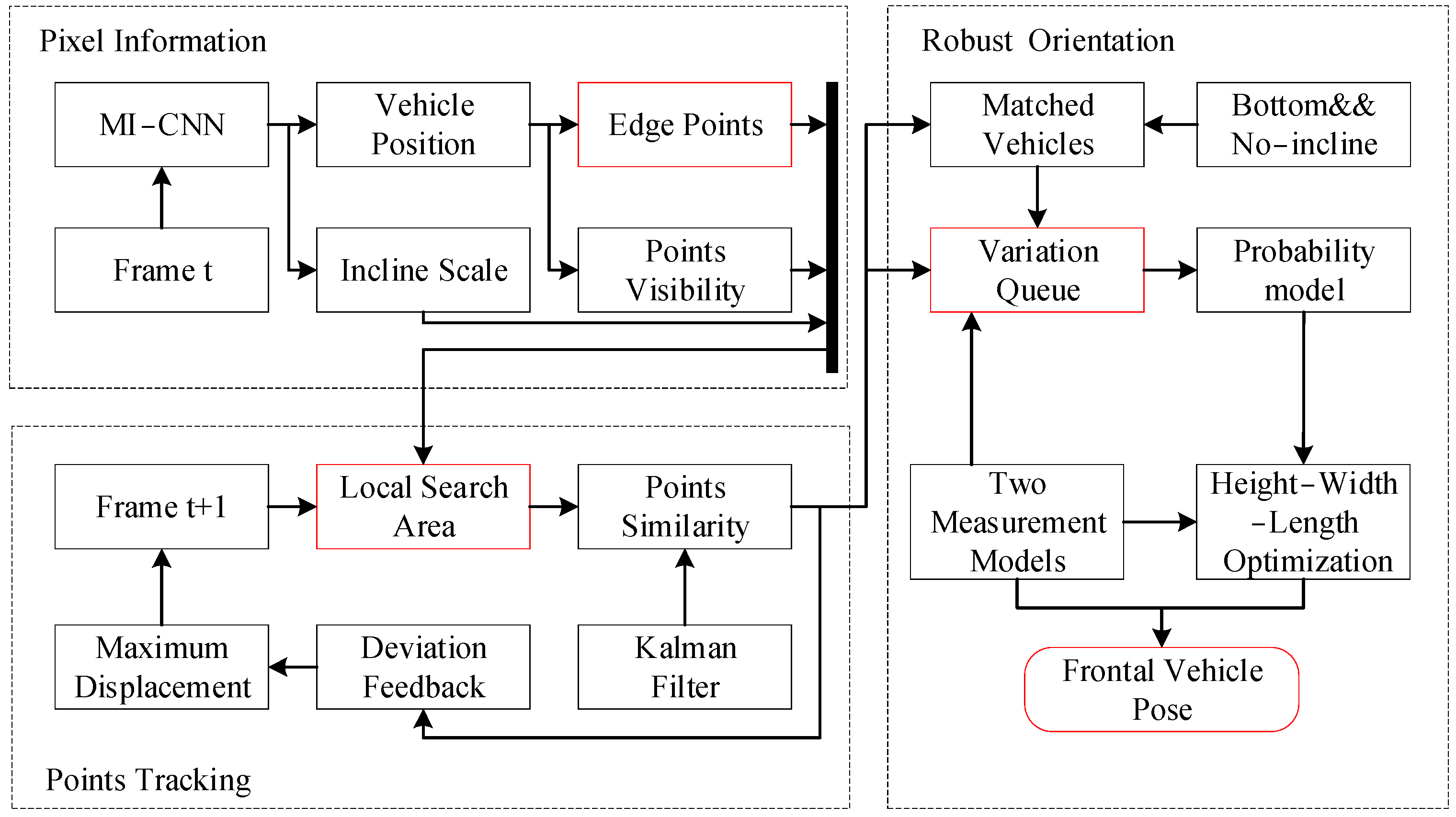
The comprehensive framework for vehicle pose estimation is depicted in Figure 2. The process consists of three subsystems: pixel information, point tracking, and robust orientation. The pixel information subsystem represents the extraction of information such as vehicle position and edge points from video frames. The point tracking subsystem is used to identify and track the movement of feature points on the vehicle over time. The robust orientation subsystem is used to evaluate and determine the direction of vehicle travel. The first process commences with the utilization of the convolutional neural network (MI−CNN) operating within a two−step detection paradigm, wherein it takes the initial frame (t) as input. This network serves a multi-faceted purpose: It simultaneously forecasts the positions of all vehicles along with their respective yaw angles relative to the host vehicle. Additionally, it is entrusted with the task of ascertaining the coordinates of edge points within the context of each vehicle’s 2D bounding box while also evaluating their visibility. The subsequent stage unfolds in frame t + 1, whereby the local search area for each vehicle is generated via a maximum displacement prediction model, incorporating an auxiliary variable. Within this search area, a fusion of edge point similarity and Kalman filter−predicted values is employed to align with the target vehicle. This matching process is instrumental in refining the redundant variable using the outcomes obtained from the match. Following the persistent tracking of the target vehicle for a span exceeding 10 frames, vehicles devoid of inclination are enlisted to compute a sequence detailing changes in distance. This sequence is established using the bottom edge as a reference point. The stability of this sequence is evaluated by means of a Gaussian distribution, which is applied with a fixed vehicle width. Once this distribution attains a state of stability, the structural parameters of the target vehicle can be refined using the aforementioned distance sequence. Consequently, this refined information facilitates the estimation of the vehicle’s pose.

3.1. Multi−Layer Edge Points of Frontal Vehicle

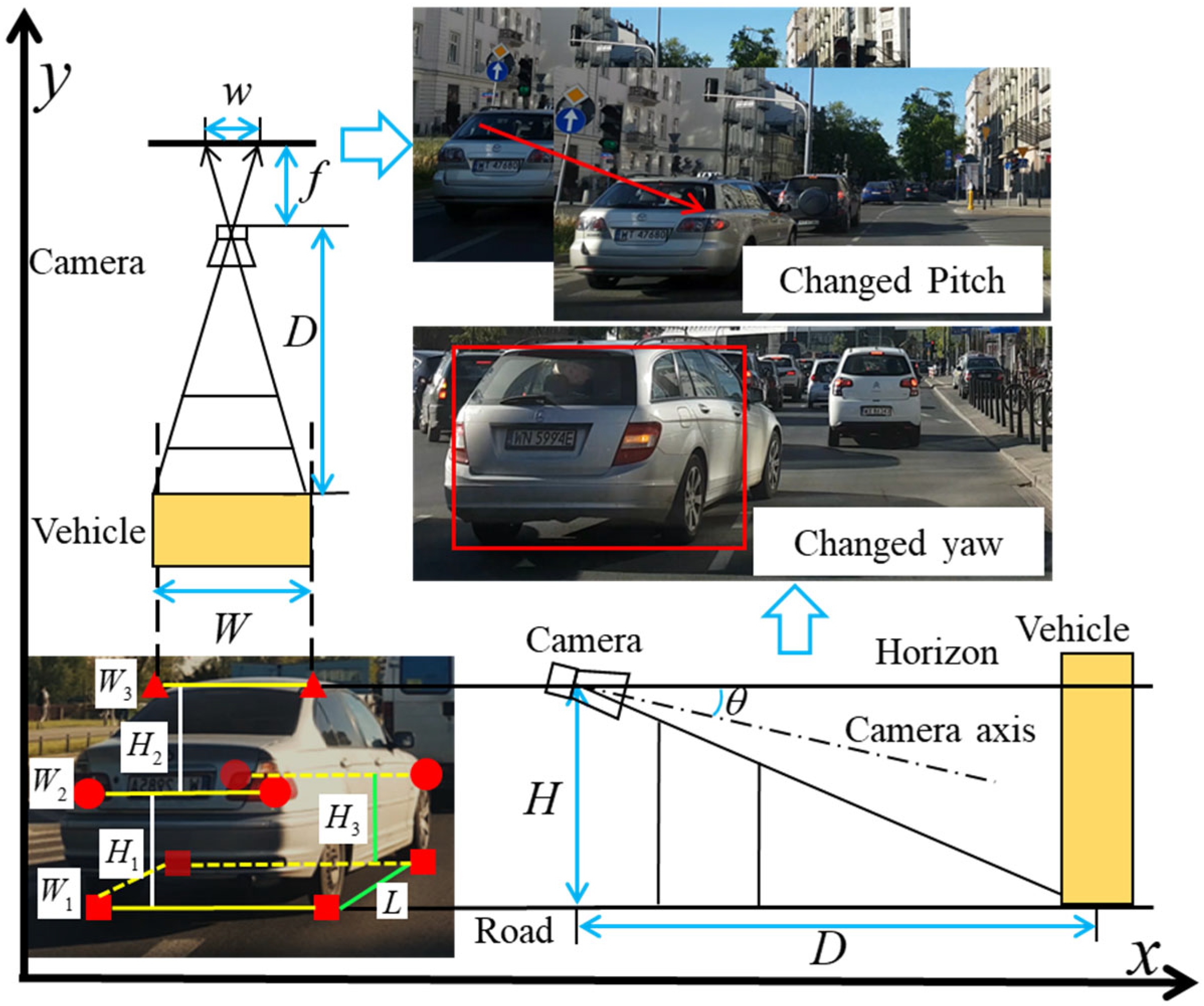
A total of ten edge feature points are encompassed within the framework, spanning various critical locations. These include the left and right contact points between the front and rear wheels and the ground, as well as two edge points positioned at the rear light of the vehicle. Furthermore, two edge points reside on the vehicle’s roof, with an additional two on the apex of the front wheel. Notably, eight of these points are directly discernible in Figure 3. When the camera pitch angle is fixed, the longitudinal distance D₁ can be measured according to the height difference between the camera and the reference point. The calculation is as follows:

$$D_1=\frac{H_i}{\tan (\arctan (\frac{\left|v-v_0\right|}{f})+\theta )}+k$$

(1)

In Equation (1), f is the focal length of the camera; v and v₀ are pixel coordinates corresponding to the edge point and the center of the optical axis, respectively; and k is the offset value relative to the selected calibration area. Let k = 0 when H_i corresponds to the bottom edge point. Other edge points can provide reliable pixel information for the distance measurement model when bottom points are invisible or blurred, but D₁ is greatly affected by the change in camera pitch angle.

When the frontal vehicle’s slant I_c relative to the camera is horizontal, the vehicle distance D₂ can be measured according to the actual width W_i between the left and right edge points on the same layer. The calculation is as follows:

$$D_2=\frac{f{W}_i}{w}+k$$

(2)

where w is the pixel width corresponding to the edge points of each layer. D₂ will not be affected by the pitch−angle change, so it is complementary to Equation (1).

After obtaining an accurate D₂, the camera pitch angle θ can be reversely calculated with Equation (1), and then the target vehicle’s yaw angle α can be calculated as follows:

$$\alpha =\arcsin (\frac{D_1^f-D_1^r}{L})$$

(3)

where f indicates the front wheel and r indicates the rear wheel. $D_1^f$ is the distance between the camera and the front wheel that has been corrected by θ, and $D_1^r$ is the distance between the camera and the rear wheel. L is the distance between the front and rear wheels. Both sets of formulas presented necessitate two essential inputs: the pixel−position data for the edge points and the unchanging rigid structural parameters pertaining to the target vehicle. The former can be predicted through the utilization of a convolutional neural network, harnessing its predictive capabilities. Meanwhile, the latter can be refined and optimized within the context of an ongoing tracking sequence, allowing for the iterative enhancement of accuracy.

3.2. MI−CNN

The MI−CNN network introduced within this paper undertakes a cohesive approach by concurrently executing four critical tasks: frontal vehicle detection, edge point localization, visibility assessment for points, and prediction of yaw angles. The fundamental network structure serves the purpose of extracting hierarchical shared features, a pivotal determinant influencing the model’s overall performance. The foundation of the network architecture is established through the utilization of residual convolution modules RI and RC [26]. These modules are fortified with short, quick connections, as visually depicted in Figure 4.

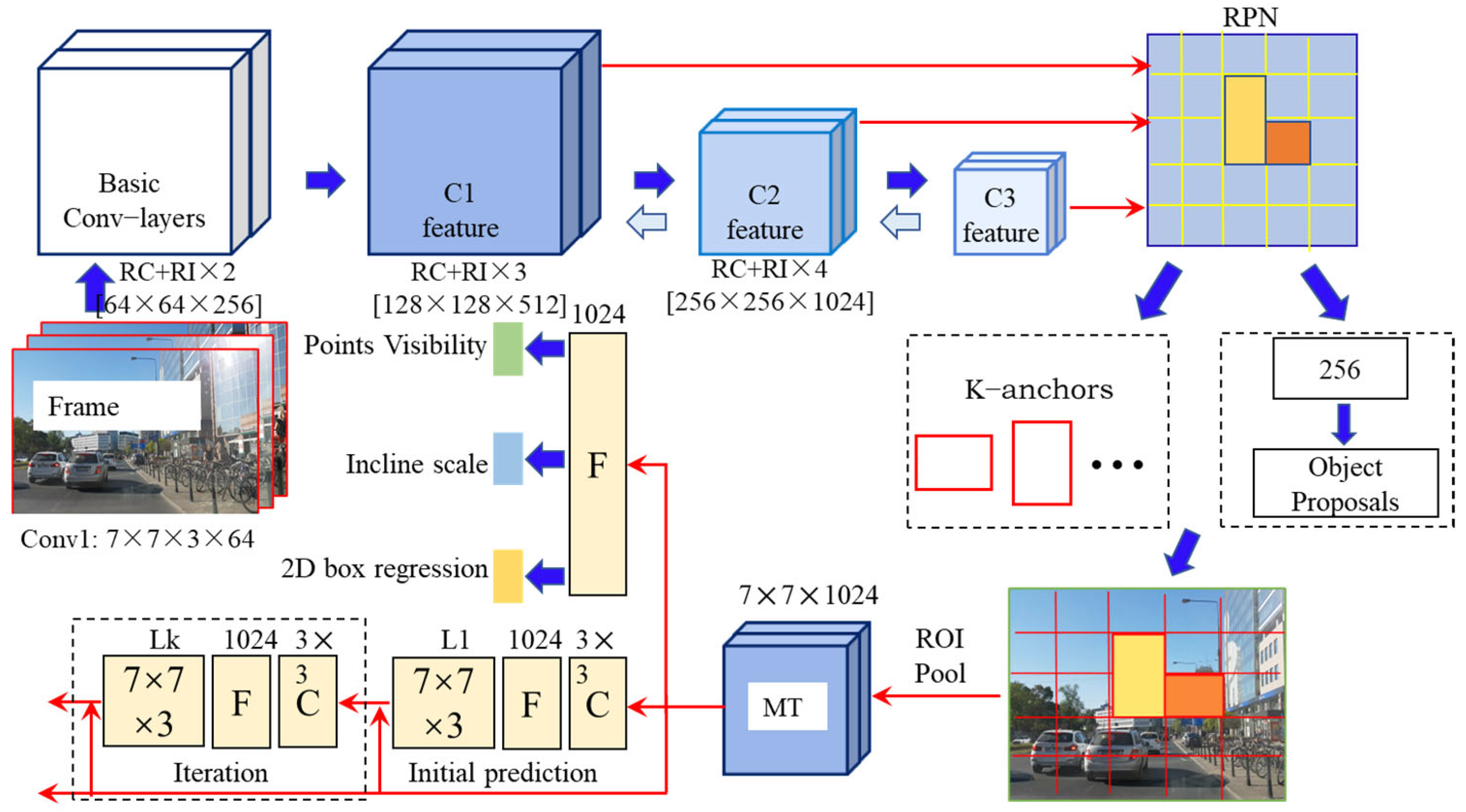
The initial layer of the network employs 7 × 7 × 3 × 64 convolution kernels with a stride of 2. Following batch regularization and pooling, it generates the initial features. Subsequently, the second layer incorporates one RC model and two RI models, each comprising a convolution kernel count of [64, 64, 256]. This stage yields a feature map denoted as C1. Advancing to the third layer, an additional RI model is introduced, increasing the convolution kernel count to [128, 128, 512]. The resultant output at this stage is marked as C2. The fourth layer incorporates another RI model while doubling the convolution kernel count to [256, 256, 1024]. Given that the feature scale has been reduced to a quarter of its original size, it becomes imperative to append a sufficient number of extraction channels to ensure the preservation of image details at all levels. The resultant shared feature map at the apex of the hierarchy is designated as C3. The ultimate step involves the combination of vehicle feature maps from distinct levels, achieved through the up−sampling operation. This amalgamation caters to the varied feature−level requirements inherent in each task.

The task of accurately locating points presents challenges when attempting to attain precise positions without initial coordinates. To enhance the network’s precision, an iterative prediction strategy is employed. This approach involves refining accuracy through a sequence of iterative predictions. In the initial prediction of the edge point coordinates {x, y, x, y} on the target vehicle, these coordinates can be rearranged into the format of a 7 × 7 × 3 feature map. This reorganized representation is then combined with the original 7 × 7 × 1024 feature map, forming an integrated input for subsequent iterations. This iterative process is iterated K times. With each iteration, the predicted coordinates of the edge points progressively converge towards more accurate values, building upon the improvements achieved in the previous iterations. In the initial iteration, a single convolutional layer and a fully connected layer, both comprising 1024 kernels of dimensions 3 × 3 × 1024, were employed. The sliding step was set to 1 to facilitate this operation. In the following iterations, the dimensions of the convolution kernels remained consistent at 3 × 3, but their count was augmented by 10 to account for the additional 10 point coordinates. The experimental observations revealed that the branch network achieved superior outcomes in terms of both localization speed and accuracy when utilizing K = 3 iterations.

The holistic architecture of the convolutional neural network, referred to as MI−CNN, is visually presented in Figure 5. Commencing with the initial RGB image as input, the foundational feature extraction network orchestrates a reverse progression. This entails infusing high−level features back into the shallow map through up−sampling. Subsequently, this process culminates in the creation of the shared feature maps, spanning three distinct stages {C₁, C₂, C₃}. ROI pooling discretizes features of candidate regions generated by the Region Proposal Network (RPN) into a fixed size and maps them to a shared task layer MT using 3 × 3 kernels. The column vector (1024) scaled from MT is used to calculate the bounding box coordinates B_i, point visibility V_i, and initialization yaw angle I_i of the frontal vehicle. $I_i\in (0,1)$ represents the applicable range of the width−ranging model, in which I_i = 0 indicates that the frontal vehicle is completely flush with the host and I_i = 1 indicates it is changing lanes or turning. The point location task first calculates the primary coordinates of the ten edge points $P_i^1={(L_j^1,R_j^1)}_{j\in \{1,2,3\}}$ through a series of 3 × 3 convolutions, a 1024 full−connection layer, and a regression layer. Then, these coordinates and MT are spliced together to be input for the next prediction.

In this paper, the convolutional neural network MI−CNN contains five loss functions that need to be optimized, namely L_rpn, L_dec, L_points, L_lic, and L_dec, which are loss functions of the RPN network and vehicle detection task. Respectively, the calculation process is the same as [1], and L_point is the loss function of the edge point position task.

Given that the precision of forthcoming vehicle distance measurements is intricately linked to the horizontal pixel separation between the left and right edge points located within the same layer, this study shifts its emphasis. Instead of singularly refining the position of individual edge points, this paper adopts a fresh approach: prioritizing the minimization of ranging errors directly. Through joint optimization, the adjacent left and right points within the same layer are regarded as an integrated unit. Suppose the true coordinates P of layer i are P_i = {x₁, y₁, x₂, y₂} and the 2D bounding box is {x, y, w, h}; then, its normalized coordinates are:

$$\overline{P_i}=\{\frac{x_1-x}{w},\frac{y_1-y}{h},\frac{x_2-x}{w},\frac{y_2-y}{h}\}$$

(4)

where $P_{\ast }^t$ represents the normalized coordinates of the edge points. Let ϕ^t indicate the mapping function of the convolutional network in iteration t, T be the shared feature map, and $P_{*}^{t-1}$ be the normalized coordinates of the edge points from the previous prediction; then, the prediction output of the positioning branch network in iteration t is:

$$P_{\ast }^t={\varphi }^t(T,P_{\ast }^{t-1}), t\ge 2$$

(5)

The loss function L_points of this layer can be calculated as follows:

$$L_{points}={\lambda }_{points}B(R(\overline{P_i}-P_{\ast }^t)+\frac{\Delta x}{w}+\frac{\Delta y}{h})$$

(6)

where $\lambda$ represents the equilibrium coefficient of the point positioning loss function, $B$ indicates whether the current region contains the target vehicle, R represents the robust L1 loss function in [11], and $\Delta x$ and $\Delta y$ denote, respectively, the width and longitudinal distance error corresponding to one point pair. $L_{vis}$ is the visibility judgment loss function. Given the true visibility vector $\overline{V}$ (corresponding to ten edge points in the target area) and the network prediction vector $V_{*}$, the loss function can be calculated as follows:

$$L_{vis}={\lambda }_{vis}B(P(\overline{V},V_{\ast }))$$

(7)

where ${\lambda }_{vis}$ represents the equilibrium coefficient of the visibility judgment loss function and $P$ is the standard softmax loss function.

L_lic is the loss function for predicting the frontal vehicle’s yaw angle, which will set I_i to 0 when the frontal target is parallel to the host. Given the true yaw angle of the target vehicle $\overline{I}$ and the predicted value of the network $I_{*}$, the function is calculated as follows:

$$L_{lic}={\lambda }_{lic}B(R(I_{*}-\overline{I}))$$

(8)

where ${\lambda }_{lic}$ represents the equilibrium coefficient of the loss function L_lic. When the candidate vehicle region does not contain the target, i.e., B = 0, all the above loss functions are null, and meaningless optimization will no longer count.

3.3. Point Tracking Based on Local Search Area

Tracking edge points form the foundational basis for calculating the unknown structural parameters delineated in Equations (1)–(3). Given that MI−CNN effectively identifies the frontal vehicle and its corresponding edge points within each frame, this section of the paper is dedicated to elucidating the optimal approach for inter-frame matching.

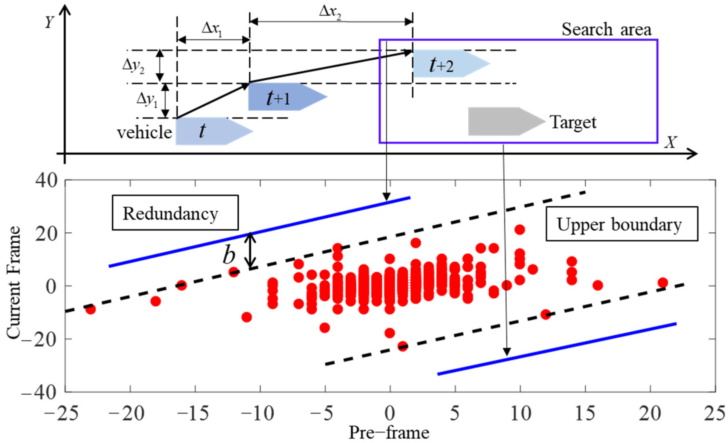
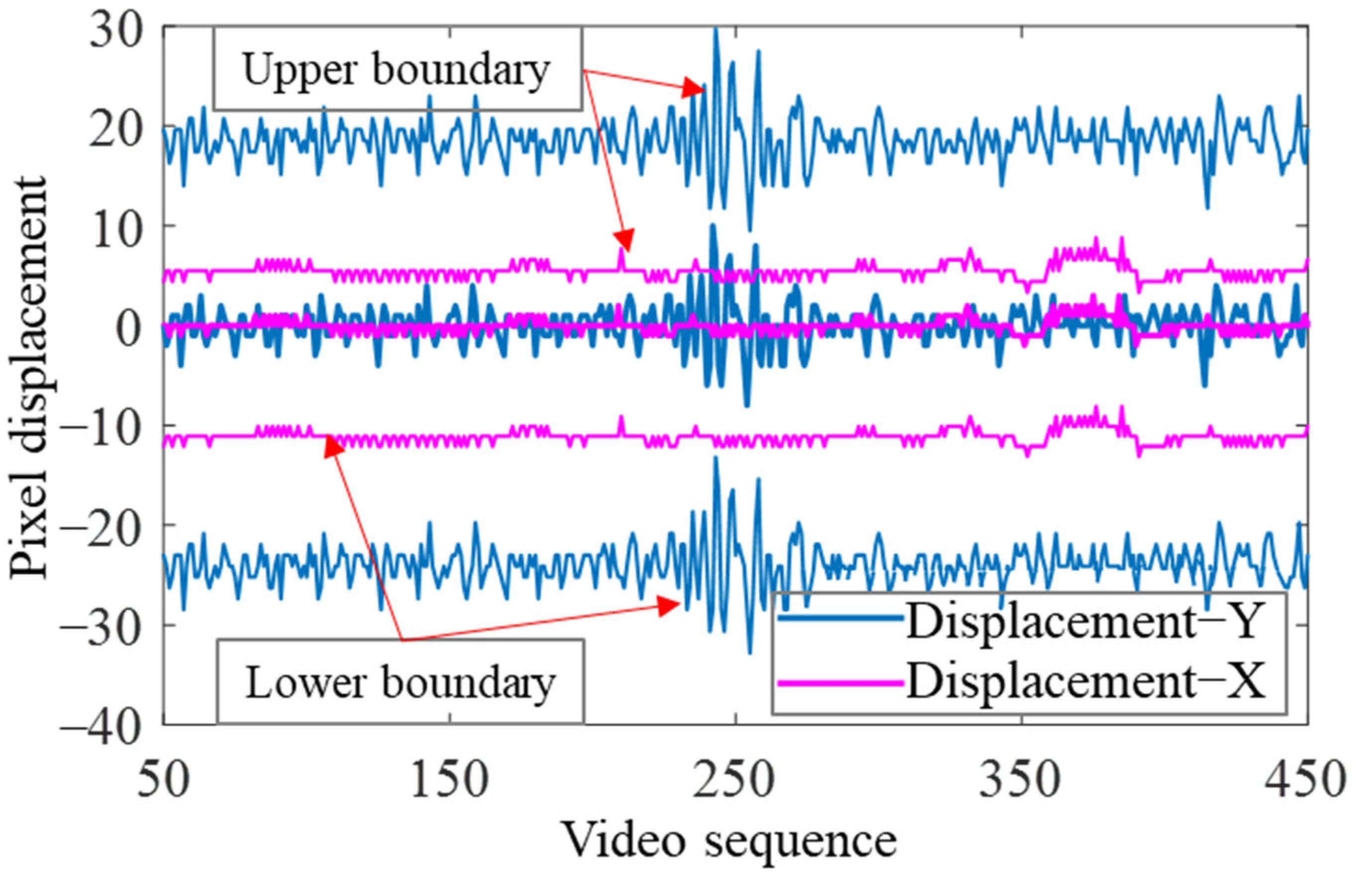
In scenarios characterized by high video frame rates, the intervals between frames translate to minimal inter−vehicle distances, resulting in relatively minor changes in pixel displacement within the image. Consequently, the conventional practice of globally matching target vehicles on a one−by−one basis is deemed unnecessary [27]. The decomposition of motion and the statistical analysis of pixel displacement for select frontal vehicles across frames are vividly depicted in Figure 6. The abscissa represents the frontal vehicles’ pixel displacement component in the horizontal or vertical directions in the previous frame (Δx₁ or Δy₁), while the ordinate represents the displacement component of the current frame (Δx₂ or Δy₂). In Figure 5, the dotted black lines demarcate the upper and lower envelopes of the scatter diagram. The range R delineated by the black dashed lines defines the local tracking search area, meticulously aligning with the prerequisites of vehicle matching. Given the inherent limitations of prior datasets to encompass the entirety of working conditions, a redundant variable b is introduced. This variable dynamically adjusts the search area in real time, guaranteeing continuous adequacy for R to encompass the upcoming target.

Suppose the resolved motion of the frontal vehicle is approximately equal to the linear motion with uniform speed. In that case, Δy_pre is the displacement of the previous frame, a is the acceleration, and Δt is the fixed inter−frame time; then, the current displacement Δy is:

$$\Delta y=\Delta y_{pre}+a\Delta t^2$$

(9)

Due to the interference caused by system delays, measurement errors, or other factors, a linear fitting model of the local tracking search area can be established according to Equation (3):

$$\Delta y=k_1\Delta y_{pre}+k_2+b$$

(10)

where k₁ and k₂ can be obtained after fitting the scatter plot data, and b can be corrected with the calculated redundancy distance after vehicle matching. It will keep the redundancy constant.

When the tracking search areas overlap with each other or the number of vehicles to be matched is greater than one, the optimal matching association can be obtained by combining motion and texture similarity. Given that the number of vehicles in the current search area is N₁, M_i,j = 1 represents that vehicle I in frame t matches vehicle j in frame t + 1, while M_i,j = 0 represents that they do not match. The set $\Delta =\{M_{i,j}\}\in {\{0,1\}}^{N\times N}$ represents all matching combinations, and the optimal association can be calculated as:

$${\Delta }_{\mathrm{op}}=\underset{\Delta }{\arg \max }{\displaystyle \sum _{i=1}^N{\displaystyle \sum _{j=1}^N{s}_{i,j}{M}_{i,j}}}$$

(11)

$$\{\begin{array}{l}{\displaystyle {\sum }_{i=1}^N{\Delta }_{i,j}=1i\in \{1,2,\dots N\}}\hfill \\ {\displaystyle {\sum }_{j=1}^N{\Delta }_{i,j}=1}j\in \{1,2,\dots N\}\hfill \\ {\Delta }_{i,j}\in \{0,1\}\hfill \end{array}$$

(12)

where 0 is filled in when the number of vehicles is insufficient, and s_i,j represents the matching confidence between vehicles i and j. It can be calculated as follows:

$$s_{i,j}=\alpha s_{m,ij}-(1-\alpha )s_{p,ij}$$

(13)

$$\{\begin{array}{l}{s}_{m,ij}=\mathrm{a}\times \exp ^\{\frac{-d_{i,j}{}^2}{2{\sigma }^2}\}\hfill \\ s_{p,ij}={\displaystyle \sum _{i=1}^6(I_i^{t+1}-I_i^t{)}^2}\hfill \end{array}$$

(14)

where $\alpha$ is the similarity weight, $\sigma$ is the prediction variance, and s_m,ij is the motion similarity between vehicles. d_i,j is the pixel distance between the predicted vehicle with the Kalman filter and the candidate vehicle. s_p,ij is the texture similarity between edge points that can be calculated by the square of the difference (SSD). $I_i^t$ and $I_i^{t+1}$ represent the corresponding pixel between the previous and next seconds. When (i, j) belong to the same vehicle, their imaging appearance is similar, and SSD will be small; meanwhile, the corresponding confidence s_i,j will increase.

3.4. Parameter Optimization

When the current frontal and host vehicles are on the same ground and the pitch angle is fixed, the camera’s mounting height can be inserted into Equation (1) to calculate the longitudinal vehicle distance D₁, which can be used to optimize other vehicle structural parameters such as height, width, and offset. When D₁ is accurate, given that the true width of the target vehicle is $\overline{W}$, and the initial vehicle width with a certain error is W*, then Formula (2) can be calculated as:

$$\eta =\frac{\Delta D_1^i}{\Delta D_2^i}=\frac{D_1^{t+i}-D_1^t}{D_2^{t+i}-D_2^t}=\frac{\frac{f\overline{W}}{w^{t+i}}-\frac{f\overline{W}}{w^t}}{\frac{f{W}^{\ast }}{w^{t+i}}-\frac{f{W}^{\ast }}{w^t}}=\frac{\overline{W}}{W^{\ast }}$$

(15)

where $D_1^t$ and $D_1^{t+i}$ are the distances calculated by Formula (1) in frames t and t+i, and $D_2^t$ and $D_2^{t+i}$ are the distances calculated by Formula (2). When the errors in Formulas (1) and (2) are small, the ratio of the vehicle distance variation $\eta$ shall be exactly equal to the ratio between the true and initial vehicle widths. When frontal vehicles are flush with the host, that is, $I_k\approx 0$, the reliability of the current D₁ sequence is judged by the probability distribution of the $\eta$ sequence for detecting a stable reference vehicle distance to correct the initial ranging parameters.

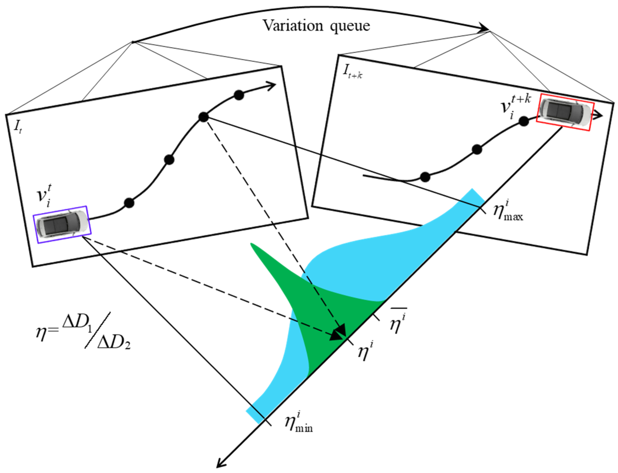
As shown in Figure 7, the distance variation sequence $\Phi ={(\Delta D_1^i,\Delta D_2^i)}_{i\in \{1,2,\dots k\}}$ is calculated in the given image sequence I_t~I_t+k. When the distribution of $\eta$ in the sequence is concentrated, it indicates that the current imaging environment is relatively stable, but if $\eta$ does not converge, the sequence will be discarded directly. After calculating the mean value $u$ and variance $\tau$ in the $\eta$ sequence that is subject to a normal distribution, the reliability of $\Phi$ can be calculated through a mixed model containing a Gaussian and a uniform distribution. When the two distance measurement models are stable, the value interval of $u$ is small and $\tau$ will approach 0:

$$p(\Phi |\epsilon ,\delta )=\delta N(\tau |0,\epsilon )+(1-\delta )U(u|u_{min},u_{max})$$

(16)

where $\delta$ is the weight of the Gaussian distribution and $\epsilon$ is the variance of $\tau$ when $\Phi$ is reliable. u_min and u_max can be set with the maximum and minimum values in the prior dataset U. By employing the aforementioned methodology, it becomes possible to efficiently filter out unforeseen sequences characterized by significant fluctuations in the distance change ratio. This proactive filtering process effectively mitigates the perturbations introduced by variations in pitch angles. Upon successfully identifying the reference distance sequences, the subsequent phase involves optimizing unknown parameters.

Given an accurate reference distance, the unknown parameters of the vehicle structure can be corrected. Assuming the true ranging sequence is $\{D_1,D_2,.D_i\dots ,D_t\}$, take Equation (2) as an example and let x = 1/w; then, the optimal vehicle width and offsets can be calculated by minimizing objective function J:

$$J={\displaystyle \sum _{i=1}^t{(fW\times x_i+k-D_i)}^2}$$

(17)

Calculate the partial derivative of J with respect to fW and k and set $A={\displaystyle \sum x_i^2}$, $B={\displaystyle \sum x_i}$, $C={{\displaystyle \sum x_{i}D}}_i$, $E={\displaystyle \sum D_i}$; then, the target parameters can be calculated as follows:

$$\{\begin{array}{c}W=\frac{(Ct-BE)/(At-B^2)}{f}\\ k=(AE-CB)/(At-B^2)\end{array}$$

(18)

Following the calculation of other structural parameters using similar techniques, a robust estimation of the distance between the camera and the edge points becomes feasible through the utilization of two measurement models. When the bottom edge points are obstructed or offer minimal texture cues, the viability of the middle or top edge points as alternatives becomes evident. In cases involving camera pitch−angle variations, the vehicle distances derived from Formula (2) provide heightened precision. Additionally, the pitch angle can be reverse−calculated using Formula (1). Ultimately, the yaw angle of the target vehicle can undergo further refinement based on the calculated values from I_c, facilitated through the application of Formula (3).

4. Experiments

Within this section, a series of comparative experiments are conducted, encompassing three key facets: vehicle detection and edge point positioning, multi−vehicle tracking, and vehicle distance measurement, including yaw angle estimation. The performance evaluation of models is undertaken through a comprehensive analysis, utilizing two benchmark datasets: the KITTI dataset and a custom−created vehicle sensing dataset. The KITTI dataset comprises 7481 training images and 7518 test images, whereas the self−constructed vehicle sensing dataset incorporates 63 training videos and 52 test videos. This self-generated dataset stems from an onboard camera situated on the front windshield. Notably, these datasets offer a rich source of vehicle samples extracted from natural driving scenarios, replete with challenging conditions such as occlusion, shadow interference, and fluctuations in illumination. This inherent complexity underscores the difficulty faced by most sensing models in accurately extracting target information within such dynamic and intricate environments.

4.1. Vehicle Detection and Edge Point Location

The convolutional neural network MI−CNN was constructed using the Keras framework. Within this network architecture, the Region Proposal Network (RPN) employed a setting where each anchor generated a pool of 70 candidate boxes [28]. These candidates were evaluated against a coincidence threshold of 0.7 for the candidate regions. Subsequent non−maximum suppression was executed with a threshold value of 0.6. For training purposes, a total of 11,677 images sourced from the two datasets were randomly selected, while the remaining images were dedicated to testing. The test platform used was a laptop computer with an Intel(R) Core i7−10700 CPU processor and two RTX−3060 GPUs. The equipment manufacturer is Dell, from Londrak, Texas, USA. The laptop computer was equipped with an Ubuntu 20.04 system. The training process was completed over approximately 23 h with GPU acceleration.

Vehicle detection forms the fundamental cornerstone for the ensuing tasks. To assess the efficacy of MI−CNN, it is rigorously compared against other contemporary state−of the−art methodologies as reported in the recent literature. The Precision–Recall (PR) curves for each method are graphically presented in Figure 8. In these curves, the abscissa corresponds to the Recall, which signifies the ratio between the number of accurately detected vehicles and the overall number of vehicles. On the ordinate, the Precision indicates the proportion of correctly identified vehicles in relation to the total network outputs.

The discernible trend in Figure 8 illustrates that the MI−CNN network boasts a higher detection accuracy when compared to the majority of prevailing vehicle detection methods. Its performance is second to the MANTA method [23], which integrates an iterative Region Proposal Network (RPN) with prior database information. This observation substantiates that the streamlined basic feature extraction network and the incorporation of the supplementary edge point localization task do not impede the object detection prowess within the dataset. Conversely, they enhance the network’s capacity to generalize effectively across diverse scenarios, resulting in improved overall detection performance. The mean Average Precision (mAP) achieved by the MI−CNN network stands at 89.9%. This figure surpasses the mAP of RSN101 by approximately 1.3%, based on the original ResNet−101 network. The distinctive strength of MI−CNN emanates from its adept fusion of rich textures and comprehensive semantic information. Through the amalgamation of shared feature maps across various levels and scales, the network is adept at capturing both intricate details and holistic context. Furthermore, the accuracy of candidate vehicle boxes can be further elevated through subsequent iterations and the optimization of the region of interest (ROI) area.

Beyond the 2D detection of vehicles, a paramount aspect is the accurate positioning of edge feature points. These points bear a direct correlation to the precision of vehicle distance measurements. In order to provide a more lucid understanding of the impact of edge point positioning on vehicle distance measurement, two distinct normalized measurement indices are formulated: the Vehicle Measurement Index (VMI) and the Height Measurement Index (HMI). VMI and HMI represent the absolute difference between 1 and the normalized ratio of the predicted and actual coordinates. Their calculation is as follows:

$$\{\begin{array}{c}VMI=\left|1-\frac{d{y}^t}{d{y}^p}\right|\\ HMI=\left|1-\frac{w^t}{w^p}\right|\end{array}$$

(19)

where dy^t and dy^p represent the longitudinal distance between the optical axis center and the edge point coordinates from network prediction and reality, respectively. w^t and w^p represent the predicted and labeled vehicle width between left and right edge points on the same layer. When the premises of the two ranging models are satisfied and the offset is 0, the normalized ranging error is:

$$\frac{D_e}{D_t}=\frac{\left|D_t-D_p\right|}{D_t}=\left|1-\frac{D_p}{D_t}\right|$$

(20)

where D_p is the vehicle distance calculated by the measurement model, and D_t is the true value. According to Equations (1) and (2), the magnitudes of VMI and HMI are exactly the same as the relative ranging error. When VMI and HMI are used as measuring indexes in the edge point location task, the influence of the positioning error on vehicle distance measurement can be intuitively revealed.

The distribution curves depicting the errors of the MI−CNN network, with K = 3, are depicted in Figure 9. The vertical axis “Frequency” denotes the ratio of edge points falling within a specific error range to the overall count. On the other hand, the “Fraction of Test Vehicles” represents the ratio of the cumulative number of detected vehicles when the error index is below a certain threshold to the total number of vehicles. Upon analysis of the figure, it becomes evident that, when employing the height parameter as the reference for distance measurement, the errors in point localization are predominantly concentrated within the range of 0.02 to 0.03. With VMI = 0.05, the ratio of the cumulative edge points is 0.95. When the width parameter is used as a reference, errors are mostly concentrated between 0.03 and 0.035. With HMI = 0.05, the cumulative ratio is 0.94. Based on the above experimental results, the point coordinate errors calculated by the MI−CNN network are mostly below 0.05, which can provide a valid input for the next distance measurement model.

4.2. Point Tracking

Diverging from conventional object trackers, which prioritize enhancing the alignment between tracking outcomes and designated labels [29], the focus of this section revolves around the acquisition of a continuous sequence of edge feature points. This sequence holds significance as it is subsequently utilized to optimize parameters in a seamless manner. To achieve accurate tracking, the fundamental requirement is that the current pixel displacement of vehicles falls within the confines of the generated tracking search area. In the context of the prior video dataset, Formula (10) is employed. This leads to determining the upper and lower coefficients for the longitudinal displacement model, equating to 1.13 and 1.09, respectively. For the lateral model, the coefficients are 1.1 and 0.98.

Illustrated in Figure 10, the true longitudinal displacement is depicted by the blue curve, while the true transverse displacement is represented by the pink curve. Notably, both of these curves are situated within the boundaries delineated by their upper and lower−fitting counterparts. This configuration is instrumental in guaranteeing that the target vehicle consistently resides within the confines of the local search area, thereby ensuring effective tracking. Furthermore, the pixel disparity between the actual and fitted displacements remains minimal, a crucial attribute that leads to a reduction in matching computations.

In this section, the missing rate (MR), misjudgment rate (FPR), and mismatching rate (MMR) from the evaluation criteria CLEAR [30] are used to quantify the multi−vehicle tracking performance. MR indicates the ratio between the tracking loss number and the total vehicle number; MMR represents the ratio between the number of vehicles that match incorrectly and the total; and FPR represents the percentage of candidate vehicles that cannot match the tracking target and the total.

To substantiate the efficacy of the proposed tracking method, which relies on the dynamically generated search area as detailed in this paper, a series of experiments were conducted. These experiments were conducted in conjunction with two alternative tracking approaches: individual Kalman tracking and feature extraction operator−based tracking [31]. The evaluation was performed within a video dataset encompassing diverse lighting conditions. The cumulative results of these experiments are presented in

Table 1. Quantitative evaluation of different tracking methods.

	Proposed Method (%)			Individual Kalman (%)			Feature-Based (%)
	MR	FPR	MMR	MR	FPR	MMR	MR	FPR	MMR
Video1	5.2	1.1	0.2	13.2	9.1	1.0	21.8	18.2	34.2
Video2	2.1	0.4	0.1	9.8	6.7	0.6	10.2	9.1	20.5
Video3	5.8	7.9	0.4	9.4	16.8	1.3	27.1	26.4	27.4
Video4	5.3	2.1	0	7.6	14.2	0.9	17.2	20.1	23.2
Video5	7.9	4.6	1.2	11.2	15.8	4.1	21.4	22.3	24.2

. The independent Kalman tracking method demonstrates a consistent ability to effectively track vehicles with relatively gradual speed changes within a confined scope. However, when traffic congestion intensifies, the tracking effectiveness diminishes steadily due to the challenges presented by erroneous matches. On the other hand, a tracker based on feature extraction and reconstruction fails to utilize the existing detection information effectively. Features extracted manually not only have poor representational ability but also add extra computation. The MR, FPR, and MMR indexes of the tracking method in this paper are all smaller than those of the other three methods. Edge point matching optimization based on local tracking search areas eliminates the need for complex calculations, unlike the previous global matching approach. Moreover, the correlation calculation of motion and appearance similarity increases target tracking stability. Only when the convolutional network’s detection result is wrong will it have certain missing and mismatched vehicles. When $\alpha$ = 0.56, a stable vehicle tracker is obtained with 96.2% average accuracy.

4.3. Orientation Estimation

Given that the accurate structural parameters of vehicles within the video dataset remain undisclosed, a pertinent methodology is employed. The geometric characteristics of the test vehicles are meticulously measured beforehand, and, subsequently, these measurements are compared against the algorithm’s outputs during experimentation. The test vehicles navigate across various scenarios, encompassing curves, intersections, and more. The derived statistical outcomes from the structural parameter estimation are summarized in

Table 2. Quantitative evaluation of parameter optimization.

Error	W1	W2	W3	H1	H2	H3	L
<0.12 m	0.940	0.921	0.937	0.972	0.953	0.942	0.932
<0.8 m	0.862	0.893	0.892	0.872	0.883	0.867	0.881

. The tabulated results provide a comprehensive overview of the algorithm’s performance in estimating structural parameters. A noteworthy observation from the table is that the proportion of estimated parameters whose errors fall below the threshold of 0.8 m consistently surpasses the 85% mark. When the error threshold is set at less than 0.12 m, the proportion of estimated parameters meeting this criterion consistently exceeds 90%. This finding substantiates the efficacy of the approach outlined in this paper, which leverages a mixed probability distribution to detect vehicle distance sequences reliably and accurately. This detection capability, in turn, lays a robust foundation for the subsequent optimization of structural parameters. In the course of the experiments, a discernible trend emerges: a higher probability associated with the distance sequence corresponds to diminished parameter estimation errors. However, this advantageous outcome is accompanied by an increased convergence time.

Subsequent to the optimization of structural parameters, the distance measurement of target vehicle components is undertaken even under challenging operational conditions. In order to gauge the method’s effectiveness, a comparison is made with two alternative measurement techniques within the same video dataset. These techniques entail shadow segmentation and external bounding box−based methods. To assess accuracy, a curve plotting the normalized ranging error along the horizontal axis and the cumulative proportion on the vertical axis is generated, as depicted in Figure 11. Remarkably, under equivalent measurement error thresholds, the method introduced in this paper consistently yields a notably higher count of vehicles compared to both the shadow segmentation and bounding box approaches. In scenarios where the shadow of the target vehicle is perturbed and becomes arduous to segment accurately, the corresponding shadow model exhibits greater errors. This phenomenon is depicted within Area A of Figure 12. When the lower edge of the target vehicle is obscured entirely, leaving the camera’s view limited to the roof, both the shadow segmentation model and the bounding box method confront difficulties in identifying the horizontal reference area. Consequently, these methods need to improve in their ability to maintain accurate measurement, which is evident in Area B of Figure 12.

In the ultimate phase of verification, an experiment is conducted to ascertain the robustness of our algorithm in the presence of vehicle turbulence. A test vehicle is driven in a straight path across a bumpy road. The traditional model relies on a single−point approach, and our hybrid model measures the distance variation between two vehicles. The outcomes of this experiment are contrasted and compared in Figure 13. The vehicle distance variation, taken about frame 200, is plotted on the vertical axis. The horizontal axis represents the corresponding frame numbers. The single−point model necessitates the assumption of a constant camera pitch angle. Consequently, when a vehicle experiences jolts or abrupt movements, this model produces unreasonable maximum or minimum vehicle distance estimates. This discrepancy is evidenced in Areas C and D of Figure 13. Unlike the single−point model, our algorithm can dynamically select the most appropriate ranging model and reference edge points, guided by the vehicle’s yaw angle and gradient information. This adaptability renders our algorithm less susceptible to the disruptive influences of vehicle turbulence or shadow interference, ultimately contributing to its superior robustness in real−world applications.

5. Conclusions

In this paper, a robust method for estimating vehicle structural parameters based on a reliable edge point sequence is introduced. Firstly, the multi−task MI−CNN network is used to detect frontal vehicles in each frame and iteratively locate the visible edge points. Meanwhile, the inclination angle between the target and host vehicles is predicted. After combining track search area generation and the maximization of the edge points’ texture similarity, the vehicle distance sequence is measured. Then, a mixed probability model is used to judge the distance sequence’s validity for restoring target structural parameters. Finally, the edge point set can be used to robustly calculate the frontal vehicle’s distance and yaw angle in various challenging environments. Subsequently, more edge points under the vehicle’s viewing field can be further analyzed to study the restoration of its complete 3D pose.