Abstract
Remote sensing involves actions to obtain information about an area located on Earth. In the Amazon region, the presence of clouds is a common occurrence, and the visualization of important terrestrial information in the image, like vegetation and temperature, can be difficult. In order to estimate land surface temperature (LST) and the normalized difference vegetation index (NDVI) from satellite images with cloud coverage, the inpainting approach will be applied to remove clouds and restore the image of the removed region. This paper proposes the use of the neural network LaMa (large mask inpainting) and the scalable model named Big LaMa for the automatic reconstruction process in satellite images. Experiments are conducted on Landsat-8 satellite images of the Amazon rainforest in the state of Acre, Brazil. To evaluate the architecture’s accuracy, the RMSE (root mean squared error), SSIM (structural similarity index) and PSNR (peak signal-to-noise ratio) metrics were used. The LST and NDVI of the reconstructed image were calculated and compared qualitatively and quantitatively, using scatter plots and the chosen metrics, respectively. The experimental results show that the Big LaMa architecture performs more effectively and robustly in restoring images in terms of visual quality. And the LaMa network shows minimal superiority for the measured metrics when addressing medium marked areas. When comparing the results achieved in NDVI and LST of the reconstructed images with real cloud coverage, great visual results were obtained with Big LaMa.
1. Introduction
Optical remote sensing systems can obtain observations of the ocean, the atmosphere and the Earth’s surface. The images available for remote sensing are mostly observed from a distance and are affected by atmospheric conditions and climatic factors, such as clouds [1]. Cloud cover alters the useful information in images, which is an adversity for subsequent image interpretation, as it can weaken or even cause the loss of essential information for analysis [2].
According to [3], depending on the application, the removal task is somewhat challenging, and there are currently some efforts to address this problem. In accordance with the data source, image-based methods can be divided into two categories: methods based on multiple images and methods based on a single image. When multiple images are used, the methods correct the brightness of cloudy pixels by fusing complementary information from other temporal images or other sensors. On the other hand, methods based on a single image are independent of the referenced data.
Among the efforts reported in the literature, the problem is treated with four types of methods: spectral-based, spatial-based, temporal-based and hybrid methods. In [4], a spectral-based method is presented for removing thin clouds in Sentinel-2A images, instruments of the European Space Agency’s (ESA’s) Copernicus mission, in which a semi-supervised method called CR-GAN-PM is proposed; the method combines generative adversarial networks (GANs) and a physical model of cloud distortion. Similarly, ref. [2] uses GANs to remove clouds from Sentinel images captured on the Google Earth platform, employing spatial-based methods. In [5], they apply spatial-based methods using convolutional neural networks (CNNs); the network is structured in two stages, one to extract cloud transparency information and the other to retrieve information from the ground surface. The authors use the L7Irish and L8SPARCS datasets from Sentinel-2 to perform the cloud-removal task. In [6], temporal-based methods are used to remove clouds in radar images from Sentinel-1 and 2. The authors create the SEN12MS-CR-TS dataset and employ it to train a network capable of reconstructing cloud-covered pixels. They also present a second approach that introduces a neural network that predicts data compromised by clouds using a time series. In [7], hybrid methods are applied employing a flexible form of spatial-based methods with deep learning structures based on GANs, allowing for the use of three arbitrary temporal images as references for the removal of dense clouds in Landsat-8 OLI and Sentinel-2 MSI images. The authors use FMask-based algorithms for cloud detection.
Some cloud removal processes use segmentation algorithms for cloud detection, such as the C Function of Mask (CFMask) algorithm [8], which is an algorithm intended to work with Landsat 7 and 8 images and which stands out for its efficiency in detecting cloud, thin cloud, clear, and some cloud shadows.
The Image Inpainting, approach aims to reconstruct images by removing unwanted information, incorporating missing information or presenting them in an imperceptible way [9]. According to [10], inpainting is a constantly evolving approach in the field of image processing capable of reconstructing images with greater efficiency in terms of the time spent on the process and the computational cost and has shown great promises in the treatment of damaged images. Although initially inpainting techniques were based on partial differential equations, their implementation with deep learning algorithms has shown significantly better results, which has led to the development of numerous approaches for image reconstruction, generation and compression [11].
Within the modern proposals for inpainting, applied to remote sensing, we can highlight the work of [12], where the data in the spatial and spectral dimensions of the image are reconstructed to minimize the reconstruction error in a prediction model, which is applied to obtain a representation much closer to the original image. In [13], an inpainting approach is proposed on a single contaminated remote sensing image by combining a modified GAN to recover affected or non-existent pixels without auxiliary information. The proposed model performed better in simple scenes compared to bilinear interpolation. Ref. [14] made a detailed literature review on some other promising methodologies for this purpose, and they also proposed a u-shaped AACNet which meets the essential characteristics and models more informative dependencies on the global range (Ada-attention) while also using gated residual blocks to restore images. In [15], a multiscale GAN-based inpainting approach is proposed and performs a reconstruction on sea surface temperature (SST) images. The approach contains two modules: the average estimation module (AEM) that performs a global constraint and avoids excessive deviation and the multi-scale anomaly decouple module (MSADM) that preserves the specificities of SST data.
Related Work
Despite the significant progress in modern inpainting systems, there are still difficulties when working with high-resolution images and when large areas need to be reconstructed. In the paper [16], the authors proposed two methods, one called LaMa (Large Mask Inpainting) and the other Big LaMa, both based on fast Fourier convolutions (FFCs), with a high receptive field perceptual loss and large training masks, differing only in their dimensions and resources. These models use the fast Fourier transform to perform reconstructions of areas covered by masks in images. The results presented show good performance when using inpainting with high-resolution images and robust behavior with large masks, which represents an excellent alternative for use in the recovery of satellite images in the presence of large areas occupied by clouds.
On the other hand, the S-NMF-EC algorithm is proposed by [1], where the information covered with clouds, and the shadows that accompany them, is retrieved using a non-negative matrix factorization (NMF) and error-correction method (S-NMF-EC). First, based on the spatio-temporal fusion model STNLFFM, the temporal difference between the cloud-free reference image and the target image contaminated with clouds is reduced. Subsequently, the cloud-free information of the target image is kept to a minimum by error correction, thus carrying out the reconstruction. The following indicators were used to evaluate the method’s cloud removal performance: peak signal-to-noise ratio (PSNR), correlation coefficient (CC), mean absolute error (MAE) and mean relative error (MRE).
Following the approach proposed in [17], with the aim of measuring the temperature and vegetation of the Earth’s surface from multispectral images, ref. [18] uses the LST and NDVI indices. The authors of this paper, in [19], carry out a study to determine heat islands and their relationship with vegetation on land using satellite images as well as the LST and NDVI indices.
Regarding the quantitative evaluation metrics, the works by [2,4,6,7,20] also adopt the indicators structural similarity (SSIM), square root of the average relative global error (ERGAS), root mean squares error (RMSE), normalized root mean squares error (NRMSE), spectral angle mapper (SAM) and universal image quality index (UIQI) to evaluate the performance of satellite image cloud removal methods. The work by [21] highlights the usefulness of the SSIM indicator in the phenoms related to the visual quality of the object’s structural details.
This article presents an approach that uses the LaMa method to recover lost information in large regions due to cloud covers in satellite images of the Amazon rainforest. As a complementary part, the Big LaMa model will also be included, as this model is a scalable version of the original model. Reconstructed images will be used to estimate the normalized difference vegetation index (NDVI) and the land surface temperature (LST). Experimental results compare the calculated indices in the original images (without the presence of masks) with those reconstructed after the introduction of synthetic clouds (masks). For this purpose, a database called Pamazon-Cloud is generated, in which the data are composed of satellite images of the city of Rio Branco in the Amazon rainforest of Brazil. In order to quantitatively validate the accuracy of the approach, the PSNR, RMSE and SSIM are used, which are metrics that can comprehensively evaluate reconstructed results in terms of content and structure. For qualitative analysis of image reconstruction, its LST and NDVI scatter plots were generated. Finally, experiments were carried out to recover information in satellite images with the presence of real clouds, using the CFMask segmentation algorithm to detect clouds in the reference images.
2. Materials and Methods
This section is divided into four subtopics that describe the methodologies used in the research. Section 2.1 describes the inpainting approach used for the reconstruction process. Section 2.2 conceptualizes the neural network implemented. Section 2.3 describes the procedures for calculating NDVI and LST. Finally, Section 2.4 provides the formulations of the evaluation metrics used.
2.1. Inpainting
The inpainting approach, proposed by [9], refers to an algorithm that performs image inpainting, in which it seeks to replicate the techniques used by professional painting restorers. The basic idea is to smoothly propagate information from the surrounding areas in isophone directions. In geometry, an isophone is a curve on an illuminated surface that connects points of equal brightness. In computer vision projects, isophones are used to optically verify the smoothness of surface connections. To use this approach, it is necessary to provide the region to be painted, and the painting is automatically carried out by the algorithm. Figure 1 shows an example of this process.
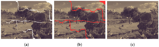
Figure 1.
Application example of the inpainting approach. (a) Image for restoration; (b) detail of areas (in red) for reconstruction; (c) reconstructed output image.
2.2. Large Mask Inpainting—LaMa
Large Mask Inpainting (LaMa) is a neural network proposed by [16] which takes into account the limitations on the receptive fields in convolutional architectures; these fields have receptor zones which, when stimulated, give rise to a response from a particular sensory neuron. LaMa is based on the theory of fast Fourier convolutions (FFCs) proposed in the work of [22], which allow for the receptive field to cover the entire image. LaMa also uses a segmentation network with a high receptive field for the perceptual losses of the image. In addition, a strategy for generating training masks is introduced in order to unlock the potential of high receptive fields.
The purpose of the LaMa network is the reconstruction of the image’s patches x, partially covered by a binary mask m of unknown pixels, generating the masked image denoted by . The m mask is stacked with the masked image , resulting in a four-channel input tensor , as illustrated in Figure 2. A feed-forward inpainting network is used, which is also called a generator. Taking , the inpainting network processes the input in a fully convolutional manner and produces a three-channel image . Training is carried out on a set of data pairs (image, mask) obtained from real images and synthetically generated masks.
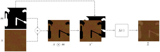
Figure 2.
Images stacking with the image x, the mask m and the resultant four-channel input tensor x.
2.2.1. Fast Fourier Convolution
FCCs are fully differentiable and are an excellent alternative to conventional convolutions due to their easy use. In addition, FCCs have receptive fields that cover the entire image, which allows the generator to notice the global context from the initial layers of the network, which is crucial for high-resolution images treated with the inpainting approach [22].
According to [16], FCC works by dividing the channels into two parallel branches. The first is the local branch, which uses conventional convolutions, and the second is the global branch, which uses the fast Fourier transform (FFT) to take into account the global context. The real FFT is applied to real-value signals, while the inverse real FFT ensures that the output is a real value. Finally, the results of the local and global branches are merged and the process is repeated until all the residual FFC blocks are completed and the image is reconstructed. The process of applying the FFC can be seen in Figure 3, where the lower output arrow of the FFC block in the flowchart refers to the result of merging the local and global branches.
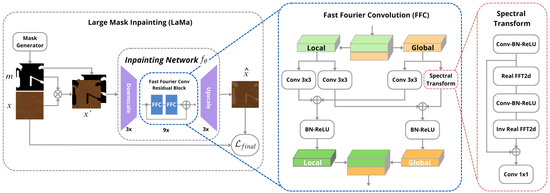
Figure 3.
The scheme of the method for large-mask inpainting (LaMa).
The LaMa network architecture has a ResNet-Like proceeding [16]. It uses three down-sampling blocks, 6–18 residual blocks and three up-sampling blocks. The residual blocks use FFC, while the discriminator architecture uses pix2pixHD, which incorporates segmentation information in object instances and allows for manipulations. They also use the Adam optimization algorithm [23], with a learning rate of 0.001 for the inpainting network and 0.0001 for the discriminator. All models are trained for 1M iterations, with a batch size between 2 and 30. The hyper-parameters were selected using the coordinate beam search strategy, resulting in , , and .
In order to obtain a better reconstruction, ref. [16] also proposed Big LaMa, a scalable LaMa model that treats real high-resolution images with large dimensions and more resources. The model differs from LaMa in three respects: the depth of the generator, the training dataset and the batch size. This model has 18 residual blocks, all based on FFC, resulting in 51 million parameters.
2.2.2. Loss Function
Loss functions are a solution to image transformation problems, where the input image is transformed into an output image from a pre-trained base network . LaMa focuses on understanding the global structure of the network layers and using a base network with rapidly growing receptive fields. Thus, the receptive field perceptual loss (HRF PL) uses a high receptive field base model given by Equation (1).
LaMa focus is shifted toward the understanding of the global structure, and it also uses a base network with rapidly growing receptive fields. This high receptive field perceptual loss (HRF PL) operates with a high receptive field base model given by Equation (1).
where is an operation that uses elements continuously, and is the average sequential operation of two phases (average between layers of the inner layers). Therefore, is implemented using Fourier.
In search of as much detail as possible, in order to have a natural effect when reconstructing images using the Inpainting model, these networks use adversarial loss, i.e., they not only learn the mapping from an input image to an output image, but also learn a loss function to train this mapping. A discriminator operates on local levels of the patches of the images, and determines the patches that are real and false, where the patches considered false are those that have an intersection with a masked area. Due to the supervised perceptual loss of the HRF, the generator rapidly learns to copy the known parts of the input image, which are labeled as “real” parts. Thus, the non-saturating adversarial loss is measured by Equations (2)–(4)
where x is a sample from the dataset, m is a synthetically generated mask, is the inpainting consequence for the , stops the gradients and is the joint loss to optimize.
The LaMa network uses differentiable training models that penalize the degree of infinitesimal change effects in the predictions. For the final loss, is used as a perceptual loss based on the discriminator; there is a perceptual loss in the characteristics of the discriminating network , which is known to stabilize the training. The final loss function for the inpainting system is the weighted sum of the losses discussed, given by Equation (5).
where and are responsible for generating local details with natural aspects, while is responsible for the supervised signal and the consistency of the global structure.
2.2.3. Masks
In LaMa, the masks play the role of clouds that result in the difficult information visualization in satellite images. Each training example is a real product of a training dataset overlaid by a synthetically generated mask.
Based on [16], the used masks represent synthetic clouds and were generated in large sizes with uniform characteristics in polygonal chains and dilated by random widths, rectangles of arbitrary proportions and thin shapes, as shown in Figure 4. The set of masks belongs to three categories: random medium masks, random thick masks and random thin masks.
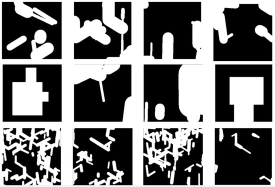
Figure 4.
Sample of masks generated to represent synthetic clouds.
2.3. NDVI and LST
According to [17,18,19], the SEBAL (Surface Energy Balance Algorithms for Land) model is used to measure the components in the energy balance instantaneously, in order to measure the flow of evapotranspiration for each pixel.
Figure 5 shows the steps taken in this analysis. From the digital satellite images, radiometric calibration is carried out to generate the reflectance for each image band, and the vegetation index and surface temperature are calculated from this reflectance.
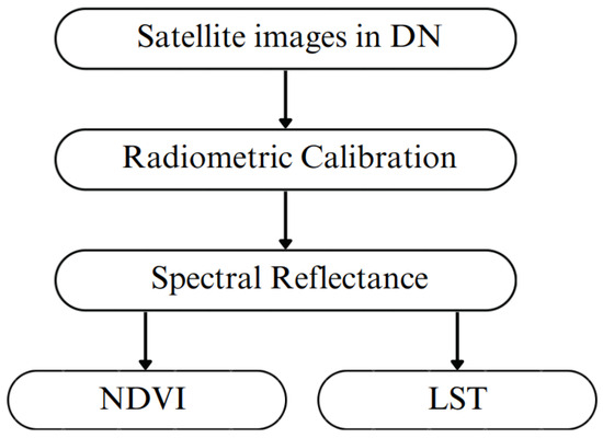
Figure 5.
SEBAL model steps used in the image processing.
2.3.1. Radiometric Calibration and Spectral Reflectance
Radiance determination begins with the generation of Level 1 (L1) products, in which the calculation of pixels with Level 0 (L0) product value, the raw value, has data converted into absolute radiance units using 32 (thirty-two) bit floating points. Subsequently, the absolute radiance values are scaled to 8-bit data and thus become calibrated digital numbers before the output to media distribution [24].
To calculate the spectral radiance of each band, the digital number (DN) of each pixel in the image is converted into monochromatic spectral radiance. This radiance represents the solar energy reflected by each pixel, per unit area, time, solid angle and wavelength, measured at Landsat satellite level. Landsat-8 satellite images only require the radiometric calibration of band 10 (thermal infrared) using Equation (6) [25].
where
= Spectral radiance in (watts/m2 × sr × μm);
= Band-specific resizing multiplicative factor;
= Quantized value calibrated by the pixel in DN;
= Band-specific additive scaling factor.
The resizing factor variables to calculate the radiance of Landsat-8 images are available in the image metadata and were applied automatically using .xml files.
The monochromatic reflectance of each band represents the ratio between the radiation flux, reflected by each band, and the incident radiation flux and is determined by Equation (7) [26].
where
= Monochromatic reflectance of each band;
Z = Sun elevation angle (degrees);
= Quantized value calibrated by the pixel in DN;
d = Inverse of the square of the relative Earth–Sun distance and the Earth–Sun distance, on a given day of the year (astronomical units);
= Multiplicative reflectance scale factor for each band.
By applying the reflectance values, it is possible to obtain the NDVI and the LST.
2.3.2. NDVI
The NDVI is an indicator that highlights vegetation and determines the relationship between the absorption of spectral radiation; in the red band, by the chlorophyll is present in plant cells, and the reflectance of leaves is found in the near infrared region. Equation (8) shows the calculation of the NDVI [27].
where
= Reflectance of the near infrared band;
= Red band reflectance.
For the Landsat-8 images, the reflectance of band 5, in the near infrared, and the reflectance of band 4, in the red, were used. We adopted five thematic classes that stipulate different types of soil situation. The NDVI intervals are identified as shown in Table 1 [28].

Table 1.
NDVI classes for land use and occupation.
2.3.3. LST
In [29], the LST calculation was defined by the ratio between the operated satellite spectral radiance in the thermal band and the emissivity, given by Equation (9).
where
= Earth’s surface temperature;
and = Calibration constants for the thermal band;
= Emissivity;
= Spectral radiance in watts/m2 × sr × μm.
The used thermal band calibration constants are available in the metadata of the captured images.
For [17], emissivity is obtained from the ratio between the energy emitted by the surface of a given material, and the energy emitted by a mass of the same temperature. Therefore, determining the emissivity of each pixel in the spectral domain in thermal band is given by Equation (10).
where
= Emissivity;
= Leaf area index.
The leaf area index is an indicator of the biomass in each image pixel; it is defined by the ratio between the leaf area of all the vegetation per unit and the area used by that vegetation. The LAI is obtained from Equation (11) [17].
where
= Leaf area index;
= Soil-adjusted vegetation index.
The SAVI is an index used to smooth out the “background” effects of the soil. It is calculated according to soil type and given by Equation (12) [30].
where
= Soil-adjusted vegetation index;
L = Adjustment factor depending on soil type.
The constant soil type (L) in the region is 0.5, because it is Latin-American soil [31].
2.4. Evaluation Metrics
PSNR is commonly used as a quality measure in the reconstruction of code with losses. Generally, the higher it is, the better its quality. For a double precision image, which has pixel values between zero and one, the PSNR is calculated according to Equation (13) [20].
The RMSE is a reference metric with clear physical meaning and easy implementation, obtained according to Equation (14) [7]:
SSIM measures the similarity between two images and assesses visual quality based on the degradation of structural information. It is calculated between two images, x and y, and given by Equation (15) [20].
3. Experiments and Results
3.1. Study Area
The Acre state, localized in the northern region of Brazil, was chosen as the study area for this research. According to the Brazilian Institute of Geography and Statistics (IBGE (https://cidades.ibge.gov.br/brasil/ac/panorama, accessed on 13 October 2023)), Acre has 830,026 inhabitants, with a population density of 5.06 inhabitants per km2, with a human development index (HDI) of 0.71, an urbanized area of 216.14 km2 and a land area of 164,173.429 km2. Figure 6 shows the study area.
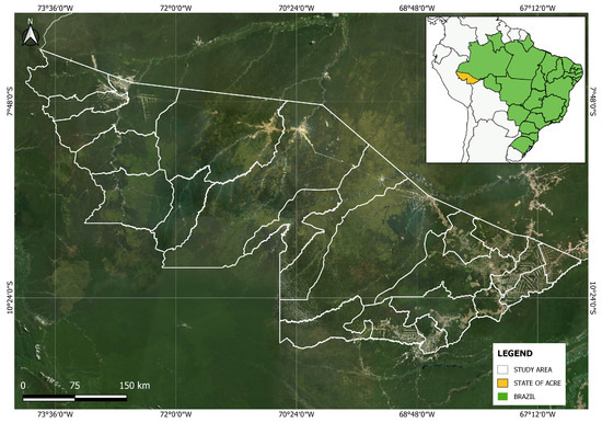
Figure 6.
Study area.
3.2. Data Acquisition
The database consists of images captured by the Landsat-8 satellite and acquired from the US Geological Survey’s online server—EarthExplorer. According to the information described in [32], Landsat products (data) are divided into UTM (Universal Transverse Mecator), WGS (World Geodetic System), OLI (Operational Land Imager) and TIRS (Thermal Infrared Sensor), wherein the size of the area pixels corresponds to 15 m in panchromatic products, 30 m in multispectral and 100 m in thermal. The data captured belong to Landsat 8—UTM and was grouped into scenes and divided into regions.
Landsat 8 sends 400 scenes per day to the USGS data archive, but is capable of regularly acquiring 725 scenes per day. The size of the Landsat 8 scene is 185 km by 180 km. The spacecraft’s nominal altitude is 705 km with an inclination of 98.2 ± 0.15. For Landsat 8 data products, a cartographic accuracy of 12 m or more is required (including compensation for terrain effects). The region analyzed belongs to the territory of the Acre state in Brazil. Figure 7 shows the scenes, in red, that mark the territory. Of all the scenes present in the study area, those with low cloud coverage were acquired and 1/67, 2/66, 2/67, 3/66, 3/67, 4/66, 4/65 and 5/66 were selected.
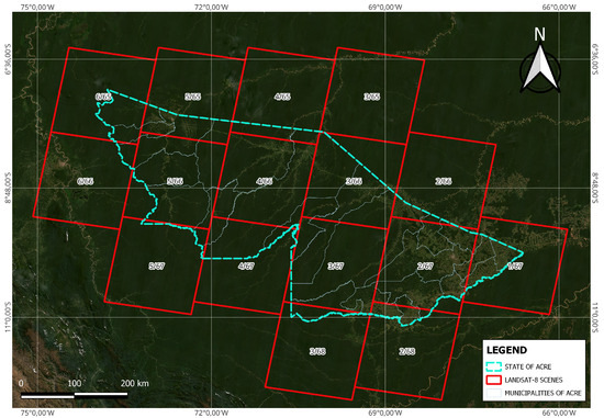
Figure 7.
Study area with Landsat-8 scenes highlighted.
Table 2 shows more detailed information on the number of images acquired for each scene and their respective year of capture.
Table 2.
Detailed information on the images acquired per scene.
The database was generated from 26 images with 7800 × 7600 pixels of resolution, covering the period between 2021 and 2023. These 26 images were selected due to the non-existence of cloud coverage. For the real data experiments, it was necessary to add a scene with cloud cover to the database.
3.3. Data Pre-Processing and Dataset Creation
Four pre-processing steps were required on the dataset in order to optimize image processing. The first stage consisted of merging the bands needed to measure LST and NDVI. The second stage involved aligning and cutting out the areas with no data. In the third stage, the image was cut into smaller patches. Finally, in the fourth and last stage, data augmentation was carried out.
In the first stage, the bands used to calculate NDVI and LST were stacked, i.e., the B4 (Red), B5 (Near Infrared—NIR) and B10 (Thermal Infrared—TIRS) bands became a single image with three channels. Figure 8 illustrates this process.
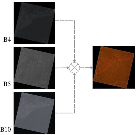
Figure 8.
Process of stacking the B4, B5 and B10 bands to generate a single image.
In the second stage, four steps were carried out to deskew the satellite images. (i) The Hough transform was used to locate the tilt angle of the images. The Hough transform [33] is a practical method for linking pixels globally and detecting curves where, from a binarization of the image, subdivisions of the plane are specified; then, the count of accumulator cells is examined for high concentrations of pixels and finally the continuity relationship between the pixels of the chosen cell is examined, thus making it possible to determine the tilt angle of the images. (ii) The image was rotated according to the angle found. (iii) The edge of the image was detected using the Canny function. The Canny approach [34] is based on three basic objectives: 1. Low error rate. All edges should be found as close as possible to the true edges; 2. The edge points should be well located. That is, the distance between a point marked as an edge by the detector and the center of the true edge must be minimal; 3. Response from a single edge point. The number of local maxima around the true edge must be minimal. This means that the detector should not identify multiple-edge pixels where only a single edge point exists. (iv) The spare region of the image was removed using the detected edge. This process is illustrated in Figure 9.
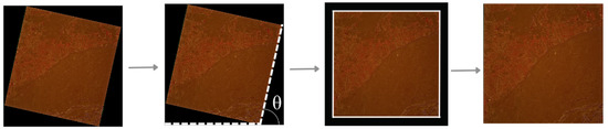
Figure 9.
Deskew applied to generate the resulting image.
In the third stage, the images were patched in order to reduce the computational cost and enable the network to learn on the available hardware. The patches were set to a size of 256 × 256 pixels, so for a captured image of 7800 × 7600 pixels, the standard size for Landsat 8 scenes, 573 patches were obtained. Thus, from the 26 images acquired, a total of 14,898 image patches were obtained. Also, 573 patches were generated from the only image with clouds for further experiments. Figure 10 illustrates this process.
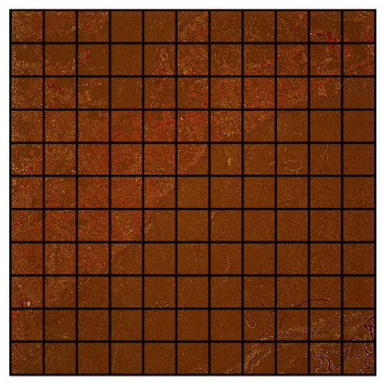
Figure 10.
Cropping applied in the images to generate patches.
The fourth and final stage consist of data augmentation, in which horizontal and vertical mirroring was performed on the patches made in stage tree, resulting in 44,646 patches, generating the dataset called PAmazon-Cloud.
The PAmazon-Cloud images were divided into three sets, one with 80% (40,646), and the other two with 10% (2000), forming the training, validation and test datasets, respectively.
3.4. Experimental Settings
The reconstructed image is used to analyze and calculate NDVI [27] and LST [29]. The approach was applied to a single reference image, and for the reconstruction of satellite images with the presence of clouds, the images are prepared with areas covered by synthetic clouds and presented as inputs. Since LaMa is based on a generator architecture Res-Net, the network selects a single reference image.
As described in Section 2.2.3, the LaMa approach uses masks to reconstruct the region of interest, and the data for training, as described in Section 2.3, are given in pairs (image, mask). For training, the masks were randomly selected to form the input pairs. The LaMa network is trained with forty epochs with a batch size of two and inputs set at 256 × 256. In addition, the Big LaMa model is trained, also with forty epochs, a batch size of two and 18 residual blocks. The hardware configuration and software environment are listed in Table 3.
Table 3.
Hardware configuration and the software environment.
In addition to visual interpretation for the qualitative evaluation analysis, three evaluation metrics were used for the quantitative analysis: root mean square error (RMSE), structural similarity (SSIM) and peak signal-to-noise ratio (PSNR), as described in Section 2.4.
3.5. Simulated Data Experiments
The PAmazon-Cloud database, described in Section 3.3, is used to carry out the approach experiments. The dataset consists of images captured by Landsat-8, duly pre-processed. The training run was limited to forty epochs and took a total of 12 days on a personal computer with characteristics detailed in Table 3. Specifically, the training process used the SSIM as an error metric to conduct the iterative adjustment to obtain the image reconstruction; the results achieved for LaMa and Big LaMa are shown in Table 4. In regard to reconstruction, it can be seen that the LaMa network and the Big LaMa model obtained their best results at epoch thirty-five, with values of 0.9802 and 0.9799, respectively.
Table 4.
Metrics achieved during training.
During the experiments, the algorithm was subjected to three types of metrics in order to evaluate performance and measure the visual quality of the image reconstruction. In the training process, the metrics were calculated for the LST due to its greater representativeness, the values of which are shown in Table 5 and Table 6. It can be seen that the LaMa network achieved the best results at epoch thirty-five, with PSNR values of 55.9807, SSIM of 0.7728 and RMSE of 0.4253. For the Big LaMa model, with thirty-eight epochs, the best PSNR, SSIM and RMSE values were 58.8912, 0.7725 and 0.1920, respectively.
Table 5.
Metrics achieved for the LST during training using the LaMa network.
Table 6.
Metrics achieved for the LST during training using the Big LaMA model.
The applicability of the approach is under in three scenarios:
- Scenario 1: The image x is contaminated with a random thick mask m and fixes multiple thick areas to be reconstructed.
- Scenario 2: In this scenario, the input image x is subjected to a random medium mask m that covers multiple medium-sized areas of reconstruction.
- Scenario 3: For this scenario, the input image x is subjected to a random thin mask m that covers multiple thin areas of reconstruction.
Figure 11 shows an image without cloud cover, which is considered the original reference image for the experiments. In the same figure, one can see their respective calculated LST and NDVI, which represent the temperature and vegetation characteristics present in the reference image. For comparison purposes, the ground truth image was considered throughout the image reconstruction process presented in this paper.
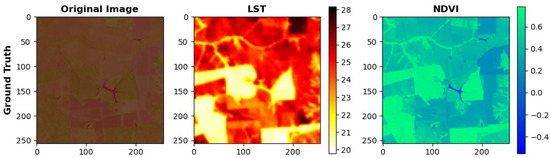
Figure 11.
The ground truth image and its respective LST and NDVI.
In order to carry out the experiments within scenarios 1 to 3 in a clear and cohesive manner, the respective mask was added to an example patch for reconstruction. Figure 12 and Figure 13 show the visual results of recovery using LaMa and Big LaMa, respectively, for each case described by the scenarios.
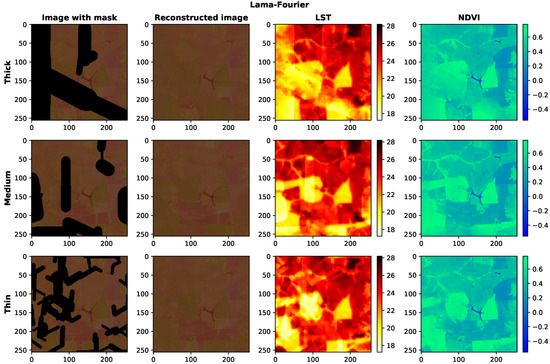
Figure 12.
Reconstruction of satellite images contaminated by synthetic clouds using the LaMa network. Each row shows images corresponding to a specific scenario and each column shows images with synthetic clouds, the reconstructed image and its LST and NDVI, respectively.
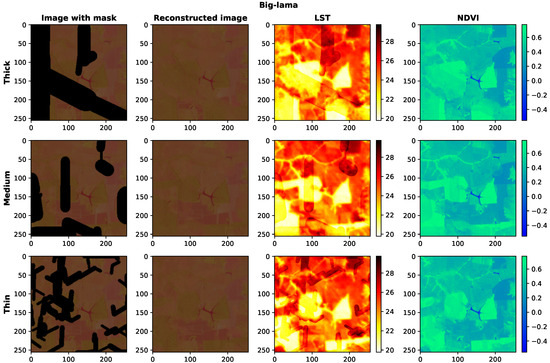
Figure 13.
Reconstruction of satellite images contaminated by synthetic clouds with the Big LaMa model. Each row shows images corresponding to a specific scenario and each column shows images with synthetic clouds, the reconstructed image and its LST and NDVI, respectively.
The first line of Figure 12 shows the result of the reconstruction in the missing areas delimited by the thick mask, characterizing scenario 1. The LST and NDVI were calculated from the reconstructed image. The second line shows the reconstruction from medium masks, scenario 2, and their respective LST and NDVI indices. The third and final line shows the reconstruction with thin masks in addition to the calculated LST and NDVI. The entire process here described was carried out using the LaMa network.
Figure 13 shows results from the Big LaMa model. Line 1, 2 and 3 of the figure show reconstructions corresponding to scenarios 1, 2 and 3, respectively. The figure also shows LST and NDVI results calculated from the reconstructed image.
Scatter plots were used to demonstrate the performance, compare and analyze the visual quality of the reconstruction with the applied approach. Representative images from scenarios 1, 2 and 3 are used to represent the scatter plots and analyze the dispersion of the reconstructed regions. Figure 14 and Figure 15 show the scatter plots for scenarios 1, 2 and 3 using LaMa and the Big LaMa model. Corresponding to scenario 1, the first lines of each figure show the behavior of the reconstructed image and its LST and NDVI. The second and third lines correspond to the results of scenarios 2 and 3, respectively. The plots consider the comparison between two variables, the average of the three bands that make up the original image without synthetic clouds and the average of the three bands that make up the reconstructed images. The resulting regions of dispersion show that the recovery carried out by the Big Lama model is clearly more concentrated, which means a higher level of consistency and precision in the reconstruction of missing areas, further highlighting its superior performance. Also, with Big Lama there is a greater strength of relationship between the variables and a higher coefficient of determination for scenario 1, representing the greater accuracy of the regression equation.
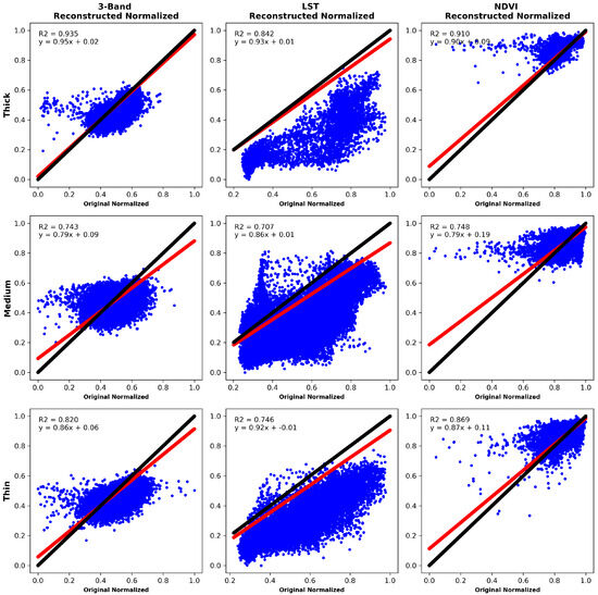
Figure 14.
LaMa network scatter plots. The black straight line represents the original image, while the red line represents the analysis of the reconstructed image versus the original image for three different scenarios. Each row corresponds to a specific scenario and each column corresponds to the reconstructed image and its LST and NDVI, respectively.
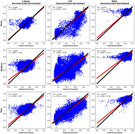
Figure 15.
Scatter plots of the image reconstruction using the Big LaMa model. The black straight line represents the original image, while the red line represents the analysis of the reconstructed image versus the original image for three different scenarios. Each row corresponds to a specific scenario and each column corresponds to the reconstructed image, its LST and NDVI, respectively.
For the quantitative analysis in the reconstruction of the example patch, PSNR, SSIM and RMSE metrics were calculated with a normalization of the reconstructed image’s data and its LST and NDVI. Table 7 and Table 8 show the results obtained by the LaMa network and the Big LaMa model in the cloud-removal task, for the Landsat data shown in Figure 12 and Figure 13.
Table 7.
LaMa implementation metrics.
Table 8.
Big LaMa implementation metrics.
From the quantitative results shown in the tables, it can be seen that, when it comes to image reconstruction and considering its visual quality as measured by the SSIM metric, the LaMa and Big Lama networks obtained better results in scenario 2, which considers medium-sized synthetic cloud cover. When it came to measuring the reconstruction of content losses, PSNR and RMSE indicators, the obtained values generally indicated a better behavior of the reconstructed image in scenario 3, which considers the coverage of synthetic clouds with thin areas. It can also be seen that there are some cases wherein better behavior is observed in scenario 2. In the reconstructed image, the best PSNR value is achieved in scenario 2 with a value of 57.1982, the best SSIM with a value of 0.9181 also for scenario 2, while the RMSE reaches 0.0075 as the best result in scenario 3. All the metrics were achieved using the LaMa network reconstruction. When the LST was analyzed, the best PSNR value was achieved in scenario 3 with a value of 48.5236 using the Big LaMa model. The best SSIM result was 0.7994 for scenario 2 using the LaMa network. The RMSE reached 0.9135 as the best result for scenario 3 using the Big LaMa model. In relation to NDVI, the best PSNR value was achieved in scenario 3 with a value of 74.3175, the SSIM with the best result of 0.8622 for scenario 2 and the RMSE reached 0.0489 as the best result for scenario 3, all of these best results using the LaMa network.
3.6. Real-Data Experiments
In order to evaluate the reconstruction from satellite images with information hidden by real clouds, new data captured by Landsat 8 were added and pre-processed (according to the steps in Section 3.3). The new data are part of scene 2/67 from September 2023 of the study area (Figure 7). This was chosen due to it being the beginning of spring and the transition from the dry season to the rainy season in the region, according to the National Institute of Meteorology (INMET (https://portal.inmet.gov.br/paginas/estacoes, accessed on 13 October 2023). To delimit the areas with clouds and their shadows, before the reconstruction process, the clouds were segmented using the CFMask algorithm [8]. As a result of the segmentation, the m mask was generated, which will be considered as one of the inputs for the reconstruction approach, as shown in Figure 2. Figure 16 shows the original image with the presence of real clouds x, the image that results from the image with the mask from the segmentation process stacked with the masked image, the reconstructed image by LaMa and the Big LaMa model and its LST and NDVI indices, respectively.
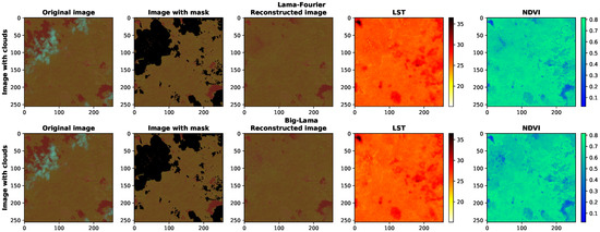
Figure 16.
Reconstruction of satellite images with cloud coverage, using LaMa and Big Lama.
In order to justify the importance of the reconstruction process for LST and NDVI analysis, the indices were calculated for the image with real cloud coverage shown in the first column of Figure 16. The index values for temperature and vegetation are shown in Figure 17.
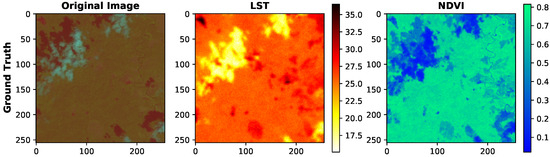
Figure 17.
The original image with clouds and their respective LST and NDVI.
4. Discussion
In the experiments carried out, satellite images captured by Landsat 8 were considered, and these images had to undergo pre-processing as described in Section 3. To simulate the presence of clouds, synthetic masks were added to the original images in order to evaluate the performance of the image reconstruction. The size of the masks characterized the scenarios for evaluating applicability: scenario 1 with thick masks, scenario 2 with medium masks and scenario 3 with thin masks.
When comparing the data from the original reference image of Figure 11 with Figure 12 and Figure 13, the results visually prove that the reconstruction carried out by the networks is adequate, as the ground truth image and those recovered by LaMa and Big LaMa have similar temperature (LST) and vegetation (NDVI) values.
In the qualitative analysis, the scatter plots shown in Figure 14 and Figure 15 describe that the recovery carried out by the Big Lama model is more concentrated, which means a higher level of consistency and precision in the reconstruction of the missing areas, highlighting its superior performance. Also, with Big Lama there is a greater strength of relationship between the variables and a higher coefficient of determination for scenario 1, representing the greater accuracy of the regression equation. This behavior may be due to its structure having more residual blocks, which may imply better efficiency in reconstructing missing areas.
Analyzing the quantitative results for the reconstructed image, shown in Table 7 and Table 8, the best performance was obtained in scenario 2, which is composed of medium-sized reconstruction areas. The PSNR and SSIM metrics indicate that the LaMa and Big LaMA approaches work well for treating satellite images with medium cloud cover. The RMSEs achieved for scenario 2 and 3 differ marginally. In relation to LST, when analyzing the SSIM metric, the LaMa network performed better for scenario 3, which corresponds to areas of thin cloud cover. Big LaMA performed better in scenario 2 when evaluating the PSNR and RMSE metrics. For NDVI, when analyzing PSNR and RMSE, the results are better for scenario 3 in both approaches. SSIM was again better for scenario 2. As a result, the visual quality of the reconstruction of images with a medium cloud cover size is higher than that of the others, which may be due to the greater preservation of contour information. As is to be expected, in scenario 3 the reconstructions were less penalized, with lower errors, due to the smaller number of pixels to be reconstructed.
It is clear that are differences between the synthetic clouds and the real clouds, so experiments were carried out on images with cloud coverage. Figure 16 shows the image reconstruction results and their respective LST and NDVI. It was found that the two algorithms achieved visually adequate results for the reconstructed image and its LST, but we can see from the NDVI in the region where the largest cloud was located that there is a difference between the results from the LaMa and Big LaMa network. According to Table 1, when the intervals in NDVI are between 0.4 and 0.6, this indicates a medium vegetation, and between 0.6 and 0.8 this indicates a dense vegetation; therefore, while examining the cloud region, the NDVI can indicate a dense vegetation for LaMa and a medium vegetation for Big LaMa. This can be harmful to remote sensing analysis.
Using the image with cloud coverage, without the reconstruction process, calculating the LST and NDVI indices can lead to an erroneous analysis. The differences in the LST and NDVI of Figure 17, compared to those of Figure 16, highlight the unrealistic information. In the LST of Figure 17, the region corresponding to the location of the cloud can be interpreted as an area with a low temperature (18 °C), an unusual characteristic for the Amazon region. This characteristic is also observed in the NDVI of Figure 17, where the cloud region can be interpreted as the existence of a flooded area, which is non-existent.
During the segmentation process, it can be seen in Figure 16 that a few cloud shadows were not properly marked, which can generate erroneous information in the LST and NDVI and lead to an inadequate analysis. As future work, the aim is to improve the cloud segmentation process in order to achieve a more detailed reconstruction of clouds and their shadows over land. Also, the authors are currently researching the use of the DM (diffusion probabilistic models) network to be used in inpainting.
5. Conclusions
Applications that analyze satellite images of indices such as NDVI and LST depend fundamentally on the seasons, i.e., they are limited to carrying out investigations in specific periods due to the presence of cloud cover blocking substantial information that can cause inconsistencies in the analysis. The innovation in the approach presented in this work is that only a single image is needed to reconstruct the areas covered by clouds in the image. It also contributes to future research into satellite image analysis that faces the same problem, since when using the proposed approach it may be possible to carry out evaluations in any season of the year.
This paper presents the reconstruction of missing parts of the Earth’s surface in satellite images with cloud cover, for the subsequent determination of the region’s vegetation and temperature levels (NDVI and LST). As a result, a dataset was created containing images of the study area, selected with as few clouds as possible. The dataset was used to train and test the LaMa and Big LaMa networks, with artificial masks representing the clouds and specifying the areas to be reconstructed. The masks represent three aspects of clouds, characterizing three scenarios: synthetic clouds covering thick, medium and thin areas. For the images that underwent the reconstruction process, the metrics PSNR, SSIM and RMSE were calculated in order to analyze whether the reconstruction was successful.
From the qualitative analysis carried out, it can be concluded that the Big LaMa model shows superior performance when compared to the results obtained by the LaMa network in the reconstruction task. On the other hand, a quantitative analysis shows minimal superiority for the metrics achieved by LaMa. From the analysis carried out, it can be seen that the reconstruction, and its respective LST and NDVI calculations, show an advantage in the values achieved in scenario 2.
Due to the differences between synthetic and real clouds, experiments with real cloud coverage were carried out, and excellent visual results were obtained, even more when compared to the alternative without the use of the implemented approach. This highlights the importance of using the image reconstruction process to analyze terrestrial features for remote sensing. When comparing the results achieved in terms of NDVI and LST for the reconstructed images, with real cloud coverage, the visual quality with Big LaMa is visibly better.
Author Contributions
Conceptualization, E.B. and A.B.A.; methodology, E.B. and A.B.A.; software, E.B., S.M., D.A.U.-F. and W.I.P.-T.; validation, E.B., S.M., D.A.U.-F. and W.I.P.-T.; formal analysis, E.B. and A.B.A.; investigation, E.B.; resources, E.B., S.M., A.B.A., D.A.U.-F., W.I.P.-T. and F.P.-Q.; data curation, E.B. and S.M.; writing—original draft preparation, E.B.; writing—review and editing, E.B., S.M., A.B.A., D.A.U.-F., W.I.P.-T. and F.P.-Q.; supervision, A.B.A. and F.P.-Q.; project administration, A.B.A. and F.P.-Q. All authors have read and agreed to the published version of the manuscript.
Funding
This research was financially supported by the PAVIC Laboratory, University of Acre, Brazil.
Institutional Review Board Statement
Not applicable.
Informed Consent Statement
Not applicable.
Data Availability Statement
The database used in this paper is PAmazonCloud, more information can be found in https://github.com/emilibezerra/cloud_painting.git, accessed on 13 October 2023.
Acknowledgments
The research was product of the colaboration between PAVIC Laboratory (Pesquisa Aplicada em Visão e Inteligência Computacional) at University of Acre, Brazil and LIECAR Laboratory (Laboratorio Institucional de Investigación, Emprendimiento e Innovación en Sistemas de Control Automático, Automatización y Robotica) at University of San Antonio Abad del Cusco UNSAAC, Perú. The authors gratefully acknowledge financial support from the PAVIC Laboratory.
Conflicts of Interest
The authors declare no conflict of interest.
References
- Li, X.; Wang, L.; Cheng, Q.; Wu, P.; Gan, W.; Fang, L. Cloud removal in remote sensing images using nonnegative matrix factorization and error correction. ISPRS J. Photogramm. Remote Sens. 2019, 148, 103–113. [Google Scholar] [CrossRef]
- Chauhan, R.; Singh, A.; Saha, S. Cloud Removal from Satellite Images. arXiv 2021, arXiv:2112.15483. [Google Scholar]
- Shen, H.; Li, H.; Qian, Y.; Zhang, L.; Yuan, Q. An effective thin cloud removal procedure for visible remote sensing images. ISPRS J. Photogramm. Remote Sens. 2014, 96, 224–235. [Google Scholar] [CrossRef]
- Li, J.; Wu, Z.; Hu, Z.; Zhang, J.; Li, M.; Mo, L.; Molinier, M. Thin cloud removal in optical remote sensing images based on generative adversarial networks and physical model of cloud distortion. ISPRS J. Photogramm. Remote Sens. 2020, 166, 373–389. [Google Scholar] [CrossRef]
- Ma, D.; Wu, R.; Xiao, D.; Sui, B. Cloud Removal from Satellite Images Using a Deep Learning Model with the Cloud-Matting Method. Remote Sens. 2023, 15, 904. [Google Scholar] [CrossRef]
- Ebel, P.; Xu, Y.; Schmitt, M.; Zhu, X.X. SEN12MS-CR-TS: A remote-sensing data set for multimodal multitemporal cloud removal. IEEE Trans. Geosci. Remote Sens. 2022, 60, 5222414. [Google Scholar] [CrossRef]
- Zhang, Y.; Ji, L.; Xu, X.; Zhang, P.; Kang, J.; Tang, H. A Flexible Spatiotemporal Thick Cloud Removal Method with Low Requirements for Reference Images. Remote Sens. 2023, 15, 4306. [Google Scholar] [CrossRef]
- Foga, S.; Scaramuzza, P.L.; Guo, S.; Zhu, Z.; Dilley, R.D., Jr.; Beckmann, T.; Schmidt, G.L.; Dwyer, J.L.; Hughes, M.J.; Laue, B. Cloud detection algorithm comparison and validation for operational Landsat data products. Remote Sens. Environ. 2017, 194, 379–390. [Google Scholar] [CrossRef]
- Bertalmio, M.; Sapiro, G.; Caselles, V.; Ballester, C. Image inpainting. In Proceedings of the 27th Annual Conference on Computer Graphics and Interactive Techniques, New Orleans, LA, USA, 23–28 July 2000; pp. 417–424. [Google Scholar]
- Mehra, S. From textural inpainting to deep generative models: An extensive survey of image inpainting techniques. Int. J. Trends Comput. Sci. 2020, 16, 35–49. [Google Scholar] [CrossRef][Green Version]
- Xiang, H.; Zou, Q.; Nawaz, M.A.; Huang, X.; Zhang, F.; Yu, H. Deep learning for image inpainting: A survey. Pattern Recognit. 2023, 134, 109046. [Google Scholar] [CrossRef]
- Amrani, N.; Serra-Sagristà, J.; Peter, P.; Weickert, J. Diffusion-based inpainting for coding remote-sensing data. IEEE Geosci. Remote Sens. Lett. 2017, 14, 1203–1207. [Google Scholar] [CrossRef]
- Lou, S.; Fan, Q.; Chen, F.; Wang, C.; Li, J. Preliminary Investigation on Single Remote Sensing Image Inpainting Through a Modified GAN. In Proceedings of the 2018 10th IAPR Workshop on Pattern Recognition in Remote Sensing (PRRS), Beijing, China, 19–20 August 2018; pp. 1–6. [Google Scholar]
- Huang, W.; Deng, Y.; Hui, S.; Wang, J. Adaptive-Attention Completing Network for Remote Sensing Image. Remote Sens. 2023, 15, 1321. [Google Scholar] [CrossRef]
- Wei, Q.; Zuo, Z.; Nie, J.; Du, J.; Diao, Y.; Ye, M.; Liang, X. Inpainting of Remote Sensing Sea Surface Temperature image with Multi-scale Physical Constraints. In Proceedings of the 2023 IEEE International Conference on Multimedia and Expo (ICME), Brisbane, Australia, 10–14 July 2023; pp. 492–497. [Google Scholar]
- Suvorov, R.; Logacheva, E.; Mashikhin, A.; Remizova, A.; Ashukha, A.; Silvestrov, A.; Kong, N.; Goka, H.; Park, K.; Lempitsky, V. Resolution-robust large mask inpainting with fourier convolutions. In Proceedings of the IEEE/CVF Winter Conference on Applications of Computer Vision, Waikoloa, HI, USA, 4–8 January 2022; pp. 2149–2159. [Google Scholar]
- Allen, R.G.; Tasumi, M.; Trezza, R.; Waters, R.; Bastiaanssen, W. Surface energy balance algorithms for land (SEBAL). Ida. Implement. Adv. Train. User’S Manual 2002, 1, 97. [Google Scholar]
- Nova, R.; Gonçalves, R.; Lima, F. Análise temporal de ilhas de calor através da temperatura de superfície e do índice de vegetação em Recife-PE, Brasil. Rev. Bras. Cartogr. 2021, 73, 598–614. [Google Scholar] [CrossRef]
- Bezerra, E.S.; Mafalda, S.; Alvarez, A.B.; Chavez, R.F.L. Análise temporal de ilhas de calor utilizando processamento de imagens de satélite: Estudo de caso Rio Branco, Acre. Rev. Bras. Computação Apl. 2023, 15, 70–78. [Google Scholar] [CrossRef]
- Darbaghshahi, F.N.; Mohammadi, M.R.; Soryani, M. Cloud removal in remote sensing images using generative adversarial networks and SAR-to-optical image translation. IEEE Trans. Geosci. Remote Sens. 2021, 60, 4105309. [Google Scholar] [CrossRef]
- Reznik, Y. Another look at SSIM image quality metric. Electron. Imaging 2023, 35, 305-1–305-7. [Google Scholar] [CrossRef]
- Chi, L.; Jiang, B.; Mu, Y. Fast fourier convolution. Adv. Neural Inf. Process. Syst. 2020, 33, 4479–4488. [Google Scholar]
- Kingma, D.P.; Ba, J. Adam: A method for stochastic optimization. arXiv 2014, arXiv:1412.6980. [Google Scholar]
- Chander, G.; Markham, B. Revised Landsat-5 TM radiometric calibration procedures and postcalibration dynamic ranges. IEEE Trans. Geosci. Remote Sens. 2003, 41, 2674–2677. [Google Scholar] [CrossRef]
- Silva, B.B.d.; Braga, A.C.; Braga, C.C.; de Oliveira, L.M.; Montenegro, S.M.; Barbosa Junior, B. Procedures for calculation of the albedo with OLI-Landsat 8 images: Application to the Brazilian semi-arid. Rev. Bras. Eng. Agrícola Ambient. 2016, 20, 3–8. [Google Scholar] [CrossRef]
- Bastiaanssen, W.G.M. Regionalization of Surface Flux Densities and Moisture Indicators in Composite Terrain: A Remote Sensing Approach under Clear Skies in Mediterranean Climates; Wageningen University and Research: Singapore, 1995. [Google Scholar]
- Purevdorj, T.; Tateishi, R.; Ishiyama, T.; Honda, Y. Relationships between percent vegetation cover and vegetation indices. Int. J. Remote Sens. 1998, 19, 3519–3535. [Google Scholar] [CrossRef]
- Bezerra, P.E.S.; Moraes, E.d.; Soares, I.d.C. Análise da Temperatura de Superfície e do Índice de Vegetação no Município de Belém na Identificação das Ilhas de Calor. Rev. Bras. Cartogr. 2018, 70, 803–818. [Google Scholar] [CrossRef]
- Bastiaanssen, W.; Bakker, M. Use of Satellite Data in Agricultural Water Management; Embrapa Semiárido: Petrolina, Brazil, 2000. [Google Scholar]
- Huete, A.R. A soil-adjusted vegetation index (SAVI). Remote Sens. Environ. 1988, 25, 295–309. [Google Scholar] [CrossRef]
- Tasumi, M. Progress in Operational Estimation of Regional Evapotranspiration Using Satellite Imagery; University of Idaho: Moscow, ID, USA, 2003. [Google Scholar]
- Irons, J.; Riebeek, H.; Loveland, T. Landsat Data Continuity Mission—Continuously Observing Your World. NASA and USGS. 2011. Available online: https://landsat.gsfc.nasa.gov/wp-content/uploads/2012/12/LDCM_Brochure_FINAL_508.pdf (accessed on 13 October 2023).
- Hough, P.V. Method and Means for Recognizing Complex Patterns. U.S. Patent 3,069,654, 18 December 1962. [Google Scholar]
- Canny, J. A computational approach to edge detection. IEEE Trans. Pattern Anal. Mach. Intell. 1986, PAMI-8, 679–698. [Google Scholar] [CrossRef]
Disclaimer/Publisher’s Note: The statements, opinions and data contained in all publications are solely those of the individual author(s) and contributor(s) and not of MDPI and/or the editor(s). MDPI and/or the editor(s) disclaim responsibility for any injury to people or property resulting from any ideas, methods, instructions or products referred to in the content. |
© 2023 by the authors. Licensee MDPI, Basel, Switzerland. This article is an open access article distributed under the terms and conditions of the Creative Commons Attribution (CC BY) license (https://creativecommons.org/licenses/by/4.0/).