Multicriteria Optimization of Lower Limb Exoskeleton Mechanism

Abstract

Typical leg exoskeletons employ open-loop kinematic chains with motors placed directly on movable joints; while this design offers flexibility, it leads to increased costs and heightened control complexity due to the high number of degrees of freedom. The use of heavy servo-motors to handle torque in active joints results in complex and bulky designs, as highlighted in the existing literature. In this analytical study, we introduced a novel synthesis method with analytical solutions provided for synthesizing the lower-limb exoskeleton. Furthermore, we proposed a mathematical model of multicriteria optimization; as a result, we obtained several lower-limb exoskeleton mechanisms comprising only six links, well-suited to the human anatomical structure, exhibit superior trajectory accuracy, efficient force transmission, satisfactory step height, and having internal transfer segment of the foot.

1. Introduction

Exoskeleton robots have found broad applications for augmenting power and aiding in rehabilitation [1,2,3,4,5,6,7]. Power augmentation is important for tasks involving heavy load transportation with limited muscle strength, while robot-assisted technologies employing upper and lower limb exoskeletons are used for rehabilitating individuals who have experienced a loss of mobility in their joints and muscles. Studying human walking apparatus and motion diagrams representing the leg movement has been useful in various fields, including the development of human prosthetics, human mimicking robots, and advancements in research areas such as biomimetics, military combat, cinematography, toys, and terrestrial and extraterrestrial exploration [7,8]. For a comprehensive overview of bipedal walking robots and exoskeletons, refer to [1,2,3,4].

Various design and control architectures of exoskeletons were summarized in the relevant references [3,5]. In recent years, various design schemes of lower limb exoskeletons aimed at achieving compact devices and meeting specific optimality criteria have been proposed [9,10,11]. Generally, the kinematic scheme of the leg exoskeleton is based on an open-loop kinematic chain with the motors mounted directly on the movable joints. Although these open kinematic chains offer greater flexibility and ease of design, their large number of degrees of freedom (DOF) contributes to increased costs and complexities in control. Using heavy servo-motors to meet significant torques generated in active joints leads to complicated and cumbersome design. The bulkiness and substantial weight of this kind of device are highlighted in [6,12].

Numerous researchers have studied the walking apparatus, demonstrating that walking patterns are measurable, predictable, and repeatable. Ref. [13] presents a passive exoskeleton with 17 DOF for load-carrying, which includes two 3 DOF ankle joints, two 2 DOF hip joints, two 1 DOF knee joints, a 1 DOF backpack, and redundant degrees of freedom at the thigh and the shank to improve the compatibility of human-machine locomotion. In [14], a mechanism has been designed for a walking robot, effectively minimizing the number of required motors, thereby contributing to reduced energy consumption. The dimensional synthesis is conducted analytically to formulate a parametric equation, and the resulting geometry of the leg mechanism is established. However, it should be noted that this mechanism is not suitable for exoskeletons due to its significant deviation in shape from that of the human leg.

Shen et al. [6,12] introduced a 1 DOF mechanism for lower limb rehabilitation exoskeletons. In [12] proposed an integrated type and dimensional synthesis method for designing compact 1 DOF planar linkages with only revolute joints and applied the method on a leg exoskeleton that can generate human gait patterns simultaneously at hip and knee joints. Reducing the number of motors resulted in decreased energy consumption. Ref. [6] reports a close match to human gait and stable hip and knee joint outputs in their prototype due to its parallel structure. The drawback of Shen’s mechanism is its use of an 8-bar-10-joint configuration; simplification would involve reducing the number of these linkages. Ref. [15] presents a leg exoskeleton consisting of a planar five-link closed linkage. The robotic system is intended for patients who have suffered strokes. The design is simple, wearable, light, and anthropomorphic in structure, and it operates with only one motor. The drawbacks mentioned in the paper include the limitation of providing mobility solely to the knee and hip joints, as well as the need for future design improvements, such as an adjustable length mechanism to accommodate patients with varying anthropometric data. In [10], the author introduced a new 1 DOF structure, allowing adjustments of mechanism links to accommodate varying human body types. However, the geometry of the novel design is bulkier. The exoskeleton is based on a seven-link mechanism and is cost-effective and easy to implement in practical activities. This leg mechanism can ensure the mobility of knee and hip joints, and the ankle joint was not considered in favor of reducing the cost. Also, the paper states that its design may require additional improvements in future developments, such as the foot shape optimization. Another study [7] focuses on the experimental and numerical study of human gait. Its results have practical applications in the design and development of human-inspired robotic structures for use in medical, assistive, or rehabilitation fields. Specifically, the study aims to investigate the flexion-extension movements of lower limb joints in humans and analyze the ground reaction forces generated during walking on force platforms.

Plecnik proposed a synthesis method for six-bar mechanisms [16], which was applied to explore one million tasks, resulting in the synthesis of one hundred and twenty-two practical linkage designs. In [17], the author presents a design procedure for Stephenson I-III six-bar linkages that is demonstrated in the design of legs. These mechanisms are advantageous for their simplicity, characterized by a reduced number of links. Although suitable for applications such as walking robots, they may not meet the requirements for exoskeletons, which demand designs that closely conform to the human anatomy while emphasizing compactness. Hence, the quest for more compact solutions in the context of exoskeletons continues.

Demonstration of a 1 DOF closed-loop mechanical linkage that can be designed to the shape and movement of a biped human walking apparatus is also presented in [18]. A single DOF eight-bar path generator that typifies the shape and motion of a human leg is proposed. However, the relative foot stride is notably small. This concept was developed by the authors in [19] towards minimizing the number of links, and a six-link leg mechanism for a biped robot was synthesized. Unfortunately, they used prismatic joints, and the foot stride is small as well. An eight-bar walking mechanism was designed in [20], but the foot path does not have a straight-line segment that will correspond to the support phase (when the foot contacts the ground).

Design and optimization of a 1 DOF eight-bar leg mechanism for a walking machine was proposed in [21]. The leg mechanism is considered to be very energy efficient, especially when walking on rough terrains. Furthermore, the mechanism requires very simple controls since a single actuator is required to drive the leg. Dynamic analysis was performed to evaluate the joint forces and crank torques of each solution, thus taking into account inertia forces in the design. However, the total design obtained was cumbersome since the mechanism was based on Theo Jansen’s straight-line generator.

The synthesis of leg mechanisms inspired by Theo Jansen’s solution has been a research topic in the last years [22,23] for its advantages regarding the reduced number of DOFs, which makes it easier to control, the scalable design, the reduced impact on the ground during walking, and because of less energy consumption. The Theo Jansen mechanism was developed in [22] considering an adaptive and controllable mechanism on irregular ground. This research sets a basis for further extension of the Theo Jansen mechanism, considering the bending of the leg linkages while turning and providing high stiffness of design. The prototype developed was tested at various speeds and torques due to the presence of the speed control system provided in an electronic system, which enables the use of the prototype for various load-handling capacities. An eight-bar leg mechanism dimensional synthesis is presented in [23] as well. Compared to the prototype, the advantage of the proposed geometric model consists of a greater step height that helps the robotic structure overcome larger obstacles.

The Klann linkage is another single DOF walking mechanism that is patented and is widely used on multi-legged robots [24,25,26,27]. The capabilities of standard non-reconfigurable quadruped Klann legs can be significantly extended by applying the method proposed in [24]. Reconfigurable legged robots based on the 1 DOF Klann mechanism are highly desired because they are effective on rough and irregular terrains, and they provide mobility in such terrain with simple control schemes. However, both Theo Jansen’s solution and Klann’s inspired leg designs are very cumbersome, especially since they cannot be used as lower limb exoskeleton since it does not fit the size limit and overall dimension restrictions. Other related works include [28,29,30,31,32,33].

Numerous optimization techniques applied for dimensional synthesis were analyzed by Shen and Allison [12], considering two major groups: gradient-based methods and evolutionary algorithms, especially genetic algorithms. These algorithms can effectively explore the solution space for a global optimum; they can also tackle geometric constraints easily. The overview of dimensional optimization methods is presented by Desai and Annigeri as well [34].

Two critical aspects of the leg mechanisms performance were chosen to be optimized by Giesbrecht [21]: minimizing the energy to improve the efficiency of the leg and lowering the requirement for larger motors and, second, maximization of the stride length. The optimization was performed using MATLAB’s optimization toolbox. However, the goals of this work were not only the optimization but also to show that mechanism design should be considered for optimizations of a leg mechanism because they offer more control over the outcome of each solution and eliminate the analysis of impossible mechanisms that would otherwise be analyzed. The comparison between the trial-and-error and optimization results demonstrates an excellent improvement in the performance of the mechanism. The mechanism design theory was found to be an excellent tool for determining the link lengths when incorporated into the optimization because it offers greater control over the outcome of each solution. However, the final design of the leg in this work is very huge as well.

A comprehensive study of optimization-based dimensional synthesis of leg mechanisms presented by Tsuge [34]. The author showed that existing global optimization techniques rely on a random initial population and do not yield feasible designs. A new global optimization procedure, called homotopy-directed optimization, was proposed, which combines the distribution of initial solutions with gradient-based optimization: it selects initial linkage designs that solve the synthesis equations and uses gradient optimization with design refinement to obtain feasible designs. The minimization problem for each starting linkage was completed using Mathematica’s built-in optimization algorithms. However, the accuracy of a generated straight-line segment of foot path is poor, and the relative horizontal velocity of the foot is not constant.

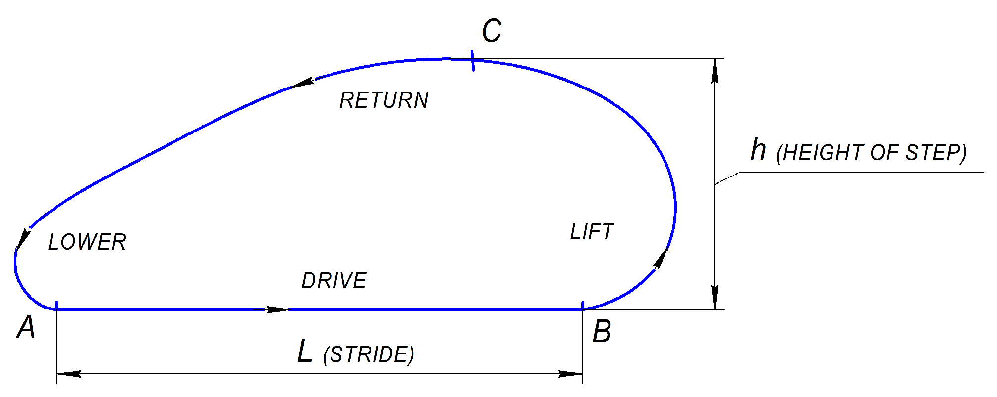
The desired foot trajectory consists of two segments (Figure 1):

• straight-line segment $A-B$ with stride L, corresponding to the support phase of step cycle (when the foot P is on the ground);
• swing phase segment $B-C-A$ with a step height h (the leg transfer phase).

In [34] presented 6 configurations of an 8-bar leg mechanism, with three fixed pivots that make it strong and stable, validated on an experimental prototype. The paper emphasizes that this mechanism offers the largest stride-to-size ratio, allowing for the construction of a compact and lightweight walking mechanism with low inertia. Consequently, it is well-suited for speed walking.

In this study, we synthesized a mechanism that is even more compact, comprising only six links. We introduced a novel synthesis method, and as the result of multicriteria optimization, we achieved a compact solution matching human anatomy with high accuracy of trajectory generation, optimized force transfer, minimized chassis height, and internal transfer of foot. This research aimed to overcome the gaps identified in prior studies, as the existing studies are focused on a single criterion, which is the accuracy of desired path generation, except for the few works mentioned above. Many authors considered multi-objective gait optimization; however, our study concerns dimensional synthesis.

This paper is organized as follows. Section 2 introduces the structure of the lower-limb exoskeleton mechanism and mathematical formulation of the synthesis problem, considering the kinematic criterion—the minimization of the accuracy of the desired output trajectory. Section 3 presents the method of kinematic synthesis, and analytical solutions were obtained for the kinematic synthesis problem. In Section 2 and Section 3, only the main design criterion—kinematic criterion was considered. Further, additional designing criteria are introduced in Section 4. A discussion of the applied multicriteria designing method is presented in Section 5, based on Sobol and Statnikov method [35], also known as random LP-$\tau$ sequences method. In total, six optimality criteria are employed, and optimal values of 18 design parameters (link dimensions) have to be determined. The noteworthy aspect of the provided design methodology is the following. Due to the obtained analytical solutions for the main design criterion (the accuracy), the dimensionality of the problem is reduced to 13 (from 18 variables), which means that at each variation of these 13 parameters, 5 variables are defined by simply solving 5 linear equations. Thus, in fact, we search for compromise solutions on 13 parameters.

The final design is presented in Section 6. Section 7 and Section 8 provide discussion and conclusions.

2. Lower Limb Exoskeleton Mechanism Structure and Kinematic Synthesis Problem Formulation

Human walking can be analyzed in three planes: the sagittal plane, coronal plane, and transverse plane [6,12]. Among these, the sagittal plane motion is predominant. The designed leg exoskeleton aids in hip and knee flexion/extension movements while the wearer stays in place. This practice focuses on motions within the sagittal plane. Consequently, a planar linkage with angular outputs can effectively facilitate these movements.

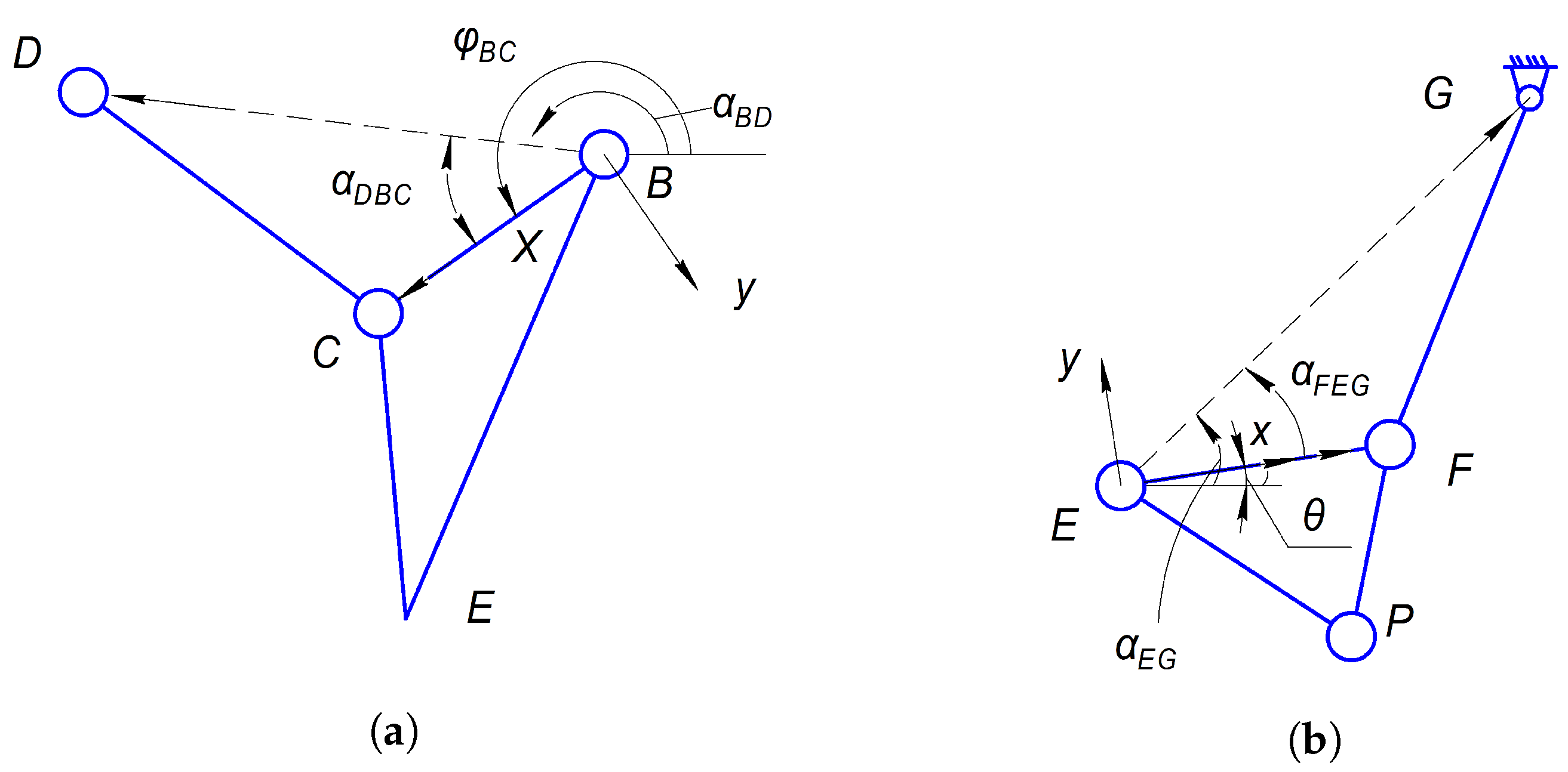
The kinematic scheme of the six-bar Stephenson III type lower-limb exoskeleton mechanism is illustrated in Figure 2a with the input link $AB$ and the foot P mounted on coupler $EF$. Rotation of the crank $AB$ is described by ${\phi }_i$,

$${\phi }_i={\phi }_0+\Delta \mathrm{\Phi }\frac{i-1}{N-1},i=\overline{1,N}.$$

(1)

$${\phi }_i={\phi }_0+\Delta \mathrm{\Phi }\frac{i-1}{N-1},i=\overline{1,N}.$$

(2)

Here, ${\phi }_0$ is an initial angular position of the crank $AB$ with respect to the horizontal axis. $\Delta \mathrm{\Phi }$ is the maximum rotation angle, $\Delta \mathrm{\Phi }>\pi$, in order to supply the overlap of support phases of alternating two legs. Kinematic analysis of the mechanism is provided in Appendix A.

The rotation of the crank $GF$ is represented by the angle ${\theta }_i$, $i=\overline{1,N}$. ${\overrightarrow{r}}_P[x_P,y_P]$ is a local radius vector, rigidly associated with the moving coordinate system $Exy$; and ${\overrightarrow{R}}_{P_i}\left[{\xi }_{P_i},{\eta }_{P_i}\right]$ and ${\overrightarrow{R}}_{E_i}\left[{\xi }_{E_i},{\eta }_{E_i}\right]$ signify the absolute positions of the foot center $P_i$ and the point E respectively. Then the relationship for ${\overrightarrow{R}}_{P_i}$ can be expressed as:

$${\overrightarrow{R}}_{P_i}={\overrightarrow{R}}_{E_i}+\mathrm{\Gamma }\left({\theta }_i\right){\overrightarrow{r}}_P=\left[\begin{array}{c}{\xi }_{E_i}\\ {\eta }_{E_i}\end{array}\right]+\left[\begin{array}{c}{x}_{P}cos{\theta }_i-y_{P}sin{\theta }_i\\ x_{P}sin{\theta }_i+y_{P}cos{\theta }_i\end{array}\right],$$

(3)

Given the desired absolute coordinates of the foot $P_i^{*}$ (Figure 2b):

$${\xi }_{P_i}^{*}={\xi }^0+L\frac{i-1}{N-1},i=\overline{1,N};$$

$${\eta }_{P_i}^{*}={\eta }^0,$$

with stride L and desired start position $P_1^{*}({\xi }^0,{\eta }^0)$, the synthesis condition is stated as follows:

$${\overrightarrow{\Delta }}_i\equiv {\overrightarrow{R}}_{P_i}-{\overrightarrow{R}}_{P_i}^{*}=\overrightarrow{0},i=\overline{1,N}.$$

(4)

Considering the constraint Equation (3) one can write in scalar form as follows:

$$\begin{array}{cc}\hfill {\delta }_i^{\xi }& =x_{P}cos{\theta }_i-y_{P}sin{\theta }_i-{\xi }^0+{\xi }_{E_i}-L\frac{i-1}{N-1}=0\hfill \\ \hfill {\delta }_i^{\eta }& =x_{P}sin{\theta }_i+y_{P}cos{\theta }_i-{\eta }^0+{\eta }_{E_i}=0\hfill \end{array}$$

(5)

Given the mechanism link lengths except ($x_P,y_P$), the synthesis task consists in determining the parameters $x_P,y_P,{\xi }^0,{\eta }^0,L$ that satisfy these $2N$ constraints approximately (since in general case we cannot meet these $2N$ Equation (5) with 5 unknowns exactly). The design parameters are:

$$x_1:=x_P,x_2:=y_P,x_3:={\xi }_0,x_4:={\eta }_0,x_5=L$$

and now the Equation (5) one can write as follows:

$$\begin{array}{c}\hfill x_{1}cos{\theta }_i-x_{2}sin{\theta }_i-x_3-x_5\frac{(i-1)}{N-1}+{\xi }_{E_i}=0\\ \hfill x_{1}sin{\theta }_i+x_{2}cos{\theta }_i-x_4+{\eta }_{E_i}=0\end{array}$$

(6)

If we introduce one more parameter $x_6=\epsilon$, which is the approximation error: $|{\delta }_i^{\xi }|\le \epsilon ,|{\delta }_i^{\eta }|\le \epsilon$, now the problem of synthesis can be stated as the following linear programming task:

$$S\left(\overrightarrow{x}\right)=x_6\to \underset{\overrightarrow{x}}{min}$$

(7)

considering constraints

$$\begin{array}{cc}\hfill & x_{1}cos{\theta }_i-x_{2}sin{\theta }_i-x_3-x_5\frac{i-1}{N-1}+x_6\le -{\xi }_{E_i}\hfill \\ \hfill & -x_{1}cos{\theta }_i+x_{2}sin{\theta }_i+x_3+x_5\frac{i-1}{N-1}+x_6\le {\xi }_{E_i}\hfill \\ \hfill & x_{1}sin{\theta }_i+x_{2}cos{\theta }_i-x_4+x_6\le -{\eta }_{E_i}\hfill \\ \hfill & -x_{1}sin{\theta }_i-x_{2}cos{\theta }_i-x_4+x_6\le {\eta }_{E_i}\hfill \end{array}$$

(8)

Using Euclidean norm for approximation error ${\overrightarrow{\Delta }}_i$, one can formulate the synthesis problem as a least-square approximation as follows:

$$S=\sum _{i=1}^N\left({\left({\delta }_i^{\xi }\right)}^2+{\left({\delta }_i^{\eta }\right)}^2\right)\to \underset{\overrightarrow{x}}{min}.$$

(9)

3. The Method of Kinematic Synthesis

3.1. Analytical Solution on 4 Synthesis Parameters

Unknown variables are:

$x_1:=x_P,x_2:=y_P,x_3:={\xi }^0,x_4:={\eta }^0$.

The conditions $\frac{\partial S}{\partial x_j}=0,j=\overline{1,4}$ lead to the following equations involving four unknowns $x_1,x_2,x_3,x_4$:

$$\sum _{i=1}^N\left({\delta }_i^{\xi }·\frac{\partial {\delta }_i^{\xi }}{\partial x_j}+{\delta }_i^{\eta }·\frac{\partial {\delta }_i^{\eta }}{\partial x_j}\right)=0,j=\overline{1,4}.$$

(10)

Namely,

$$\sum _{i=1}^N{\delta }_i^{\xi }cos{\theta }_i+\sum _{i=1}^N{\delta }_i^{\eta }sin{\theta }_i=0$$

(11)

$$-\sum _{i=1}^N{\delta }_i^{\xi }sin{\theta }_i+\sum _{i=1}^N{\delta }_i^{\eta }cos{\theta }_i=0$$

(12)

$$\sum _{i=1}^N{\delta }_i^{\xi }=0$$

(13)

$$\sum _{i=1}^N{\delta }_i^{\eta }=0.$$

(14)

Let us introduce notations:

$$\begin{array}{c}k:=\sum _{i=1}^{N}cos{\theta }_i\end{array}$$

(15a)

$$\begin{array}{c}m:=\sum _{i=1}^{N}sin{\theta }_i\end{array}$$

(15b)

$$\begin{array}{c}{b}_1:=\sum _{i=1}^N\left(-{\xi }_{E_i}+L·\frac{i-1}{N-1}\right)cos{\theta }_i-\sum _{i=1}^N{\eta }_{E_i}sin{\theta }_i\end{array}$$

(15c)

$$\begin{array}{c}{b}_2:=\sum _{i=1}^N\left({\xi }_{E_i}-L·\frac{i-1}{N-1}\right)sin{\theta }_i-\sum _{i=1}^N{\eta }_{E_i}cos{\theta }_i\end{array}$$

(15d)

$$\begin{array}{c}{b}_3:=\sum _{i=1}^N\left(-{\xi }_{E_i}+L·\frac{i-1}{N-1}\right)\end{array}$$

(15e)

$$\begin{array}{c}{b}_4:=\sum _{i=1}^N(-{\eta }_{E_i}).\end{array}$$

(15f)

Then we come to the system of linear equations expressed as follows:

$$\begin{array}{cc}\hfill & N{x}_1-k{x}_3-m{x}_4=b_1\hfill \end{array}$$

(16a)

$$\begin{array}{cc}\hfill & N{x}_2+m{x}_3-k{x}_4=b_2\hfill \end{array}$$

(16b)

$$\begin{array}{cc}\hfill & k{x}_1-m{x}_2-N{x}_3=b_3\hfill \end{array}$$

(16c)

$$\begin{array}{cc}\hfill & m{x}_1+k{x}_2-N{x}_4=b_4.\hfill \end{array}$$

(16d)

The only solution of this system in case $k^2+m^2\ne N^2$ is

$$x_1=\frac{-N{b}_1+k{b}_3+m{b}_4}{k^2+m^2-N^2}$$

(17)

$$x_2=\frac{-N{b}_2-m{b}_3+k{b}_4}{k^2+m^2-N^2}$$

(18)

$$x_3=\frac{N{b}_3-k{b}_1+m{b}_2}{k^2+m^2-N^2}$$

(19)

$$x_4=\frac{N{b}_4-m{b}_1-k{b}_2}{k^2+m^2-N^2}.$$

(20)

The necessary conditions also serve as sufficient conditions [36] for attaining the minimum of the function S: the matrix

$$\frac{d^{2}S}{d{\overrightarrow{x}}^2}=\left[\begin{array}{cccc}N& 0& -k& -m\\ 0& N& m& -k\\ -k& m& N& 0\\ -m& -k& 0& N\end{array}\right]$$

is positive-definite (in case $k^2+m^2\ne N^2$), since the determinants of all corner minors are non-negative [37]:

$$\begin{array}{cc}\hfill & {\Delta }_1=N>0,{\Delta }_2=N^2>0,{\Delta }_3=N^3+N(k^2+m^2)>0,\hfill \\ \hfill & {\Delta }_4={(k^2+m^2-N^2)}^2>0.\hfill \end{array}$$

(21)

3.2. Analytical Solution on 5 Synthesis Parameters

Let us explore a scenario where $L=x_5$ is an additional variable subject to optimization. Referring to (16a)–(16d), from the condition $\frac{\partial S}{\partial \overrightarrow{x}}=\overrightarrow{0}$ we obtain

$$N{x}_1-k{x}_3-m{x}_4-\sum _{i=1}^N\left(\frac{i-1}{N-1}cos{\theta }_i\right)x_5=b_5,$$

(22)

where

$$b_5=\sum _{i=1}^N\left(-{\xi }_{P_i}·cos{\theta }_i-{\eta }_{P_i}·sin{\theta }_i\right);$$

$$N{x}_2+m{x}_3-k{x}_4+\sum _{i=1}^N\left(\frac{i-1}{N-1}sin{\theta }_i\right)x_5=b_6,$$

(23)

where

$$b_6=\sum _{i=1}^N\left({\xi }_{P_i}·sin{\theta }_i-{\eta }_{P_i}·cos{\theta }_i\right);$$

$$k{x}_1-m{x}_2-N{x}_3-\sum _{i=1}^N\left(\frac{i-1}{N-1}\right)x_5=b_7,$$

(24)

where

$$b_7=-\sum _{i=1}^N{\xi }_{P_i};$$

$$m{x}_1+k{x}_2-N{x}_4=b_8,$$

(25)

where

$$b_8=-\sum _{i=1}^N{\eta }_{P_i}.=b_4.$$

The last equation is derived from (10), $j=5$:

$$\begin{array}{cc}\hfill & \sum \left(\frac{i-1}{N-1}cos{\theta }_i\right)x_1-\sum \left(\frac{i-1}{N-1}sin{\theta }_i\right)x_2\hfill \\ \hfill & -\sum \left(\frac{i-1}{N-1}\right)x_3+\sum \left(\frac{i-1}{N-1}{\xi }_{P_i}\right)x_4+\sum {\left(\frac{i-1}{N-1}\right)}^2{x}_5=0.\hfill \end{array}$$

(26)

Finally, taking into account

$$\sum \left(\frac{i-1}{N-1}\right)=N/2$$

(27)

and

$$\sum {\left(\frac{i-1}{N-1}\right)}^2=\frac{N(2N-1)}{6(N-1)},$$

(28)

we obtain the following system of linear equations

$$A\overrightarrow{x}=\overrightarrow{b},$$

(29)

where

$$A=\left[\begin{array}{ccccc}N& 0& -k& -m& -k_{\alpha }\\ 0& N& m& -k& k_{\beta }\\ k& -m& -N& 0& -N/2\\ m& k& 0& -N& 0\\ k_{\alpha }& -k_{\beta }& -N/2& 0& -\frac{N(2N-1)}{6(N-1)}\end{array}\right]$$

(30)

$$\overrightarrow{b}={\left[\begin{array}{ccccc}{b}_5& b_6& b_7& b_8& -k_{\mu }\end{array}\right]}^T$$

(31)

and

$$k_{\alpha }:=\sum \left(\frac{i-1}{N-1}cos{\theta }_i\right)$$

(32)

$$k_{\beta }:=\sum \left(\frac{i-1}{N-1}sin{\theta }_i\right)$$

(33)

$$k_{\mu }:=\sum \left(\frac{i-1}{N-1}{\xi }_{P_i}\right).$$

(34)

The Hessian $H_S=\frac{d^{2}S}{d{\overrightarrow{x}}^2}$, and it is non-negative definite (for the proof, refer to Appendix B).

$$H_S=\left[\begin{array}{ccccc}N& 0& -k& -m& -k_{\alpha }\\ 0& N& m& -k& k_{\beta }\\ -k& m& N& 0& N/2\\ -m& -k& 0& N& 0\\ -k_{\alpha }& k_{\beta }& N/2& 0& \frac{N(2N-1)}{6(N-1)}\end{array}\right].$$

Therefore, the last condition supplies the minimum of the function S, if $det{H}_S\ne 0$.

For analytical solution in this case we refer to Equations (16a)–(16d):

$$x_1=\frac{b_5+k{x}_3+m{x}_4+k_{\alpha }{x}_5}{N}$$

(35)

$$x_2=\frac{b_6-m{x}_{3}k{x}_4-k_{\beta }{x}_5}{N}$$

(36)

$$x_3=\frac{N{b}_7+\frac{N^2}{2}{x}_5-k{b}_5-k{k}_{\alpha }{x}_5+m{b}_6-m{k}_{\beta }{x}_5}{k^2+m^2-N^2}$$

(37)

$$x_4=\frac{N{b}_8-m{b}_5-m{k}_{\alpha }{x}_5-k{b}_6+k{k}_{\beta }{x}_5}{k^2+m^2-N^2},$$

(38)

assuming $k^2+m^2\ne N^2$; and $x_5$ can be found directly by substituting (35)–(38) into (26).

4. Additional Synthesis Conditions and Multiple Optimization Criteria

Note that when determining the solution x according to (29), the matrix A and the column vector b depend on 13 design variables $p_1,\dots ,p_{13}$ (mechanism link dimensions).

$$p_1:={\xi }_D,p_2:={\eta }_D,p_3:={\xi }_G,p_4:={\eta }_G,p_5:=r_{AB},p_6:={\phi }_0,p_7:=\mathrm{\Phi },$$

$$p_8:=L_{BC},p_9:=L_{CD},p_{10}:=x_E,p_{11}:=y_E,p_{12}:=L_{EF},p_{13}:=L_{FG},$$

where

-

${\xi }_D,{\eta }_D,{\xi }_G,{\eta }_G$ are the absolute coordinates of frame joints D and G;

-

$r_{AB}$ is the length of crank $AB$;

-

$x_E,y_E$ are the local coordinates of joint E relative to the $B{x}_2{y}_2$ moving coordinate system, with the $B{x}_2$ axis along line $BC$.

This is because ${\theta }_i,{\xi }_{E_i},{\eta }_{E_i}$ in the source Equation (5) depend on $p_1,\dots ,p_{13}$. Thereby, due to finding 5 design variables $\overrightarrow{x}=A^{-1}\left(\overrightarrow{P}\right)\overrightarrow{b}\left(\overrightarrow{P}\right)$, (that found from the kinematic requirement—generating the desired foot path; $\overrightarrow{P}$ is the vector of 13 design parameters), the dimensionality of the optimization problem is reduced to 13 design parameters instead of 18 unknowns.

However, solving Equation (29) does not provide an exact generation of the desired foot path, but supplies an approximate solution; thus, we need to improve the accuracy by using the rest 13 “non-linear” parameters. So, we have to solve the following optimization task:

$$S^0\left(\overrightarrow{P}\right)=\underset{\overrightarrow{x}}{min}S=S(\overrightarrow{P},\overrightarrow{x}\left(\overrightarrow{P}\right))=S(\overrightarrow{P},A^{-1}(\overrightarrow{P},\overrightarrow{b}\left(\overrightarrow{P}\right)))\to min.$$

(39)

However, achieving the best accuracy conflicts with some additional design requirements, such as force transmission, matching leg anatomy, etc. As the preliminary design had shown, improving the accuracy leads to worsened force transmission and decreased step height (small swing phase height limits overcoming large obstacles). Moreover, the swing phase trajectory tends to go beneath the ground level (the trajectory becomes external relative to the mechanism frame), etc. For these reasons, multiple design criteria must be considered, and a multi-criteria optimization task has to be solved. For these purposes Sobol and Statnikov method is applied [35], based on

• Generating the trial table with a great number of random LP-$\tau$ sequences of design parameters evenly distributed within the specified search area and
• Iterative approaching the compromise solutions, truncating the trial table by strengthening (“narrowing”) restrictions on criteria.

The trajectory of the foot center P called a step cycle, consists of two phases: the “support phase” and the “transfer phase” (swing). During the support phase, the foot center P should trace a horizontal straight line. The main criterion of synthesis is the accuracy of straight-line generation during the support phase, which has to be minimized:

$$c_1=\underset{i=\overline{1,N}}{max}|{\eta }_P^0-{\eta }_{P_i}|.$$

(40)

• The chassis height $H=-x_4$ has to be minimized or (which is the same condition) ${\eta }^0=-H$ to be maximized

  $$c_2=x_4.$$

  (41)
• In order to achieve the best force transmission, the worst transference angle has to be maximized

  $$c_3=\underset{0\le \phi \le 2\mathrm{\Pi }}{min}({\mu }_{BCD},{\mu }_{EFG}).$$

  (42)

  where

  $$\begin{array}{cc}\hfill {\mu }_{BCD}& =arccos\frac{L_{BC}^2+L_{CD}^2-{\left|BD\right|}^2}{2L_{BC}{L}_{CD}},\hfill \\ \hfill {\mu }_{EFG}& =arccos\frac{L_{EF}^2+L_{FG}^2-{\left|EG\right|}^2}{2L_{EF}{L}_{FG}},\hfill \end{array}$$

  (43)
  $L_{BC},L_{CD},L_{FG},L_{EF}$ are lengths of corresponding links, $\left|BD\right|,\left|EG\right|$ are distances between the centers of corresponding joints.
• In order to match human anatomy, the hip-to-shin relation $L_{FP}/L_{FG}$ (the ratio of the thigh to the lower leg) has to be around one ($c_4=1$)

  $$c_4=L_{FP}/L_{FG}$$

  (44)
• For external transfer of the foot center P, the following penalty function $c_5$ has to be minimized

  $$c_5=\sum _{i=1}^{N}max(({\eta }^0-{\eta }_{P_i}),0).$$

  (45)

The meaning of this penalty function is as follows. If ${\eta }_{P_i}<{\eta }^0$, then the penalty function $c_5$ will be increased to positive value $max(({\eta }^0-{\eta }_{P_i},0)$. Otherwise, if ${\eta }_{P_i}\le {\eta }^0$, then $max(({\eta }^0-{\eta }_{P_i}),0)=0$, thus nothing will be added to the function $c_5$.

5. Global Search and Multi-Criteria Optimization of Exoskeleton Link Dimensions

Let us keep notation $\xi ,\eta$ for absolute coordinates of joints as it was in the previous sections.

$n=13$ variable parameters of the exoskeleton mechanism are varied within a given search area by using so-called random LP-$\tau$ sequences, evenly distributed in n-dimensional parallelepiped [35,38,39]. A global search carried out specifying the following limits on variable parameters

$$\begin{array}{cc}\hfill -1.50& \le {\eta }_D\le 1.50\hfill \\ \hfill -1.50& \le {\xi }_G\le 1.50\hfill \\ \hfill -1.50& \le {\eta }_G\le 1.50\hfill \\ \hfill 0.05& \le r_{AB}\le 0.30\hfill \\ \hfill 0^{°}& \le {\varphi }_0\le {360}^{°}\hfill \\ \hfill {180}^{°}& \le \mathrm{\Phi }\le {190}^{°}\hfill \\ \hfill 0.40& \le L_{BC}\le 1.00\hfill \\ \hfill 0.40& \le L_{CD}\le 1.00\hfill \\ \hfill 0.50& \le x_E\le 1.20\hfill \\ \hfill -0.50& \le y_E\le 1.20\hfill \\ \hfill 0.10& \le L_{EF}\le 0.40\hfill \\ \hfill 0.30& \le L_{FG}\le 1.10,\hfill \end{array}$$

The foot-point traces a straight line while the crank angle is in the range ${\phi }_0\le \phi \le {\phi }_0+\Delta \mathrm{\Phi }$.

For each set of $n=13$ random variables analytical solutions for 5 design parameters $x_1,x_2,\dots ,x_5$ are determined applying Formulas (26) and (35)–(38), and the trial table is obtained by calculating design criteria values. Analyzing the obtained trial table, 25 preliminary solutions are selected as specified in

Table 1. Trial table fragment: criteria values with the limits specified by (46).

LP$\mathit{\tau }$ №	Figure	${\mathit{c}}_1$	${\mathit{c}}_2$	${\mathit{c}}_3$	${\mathit{c}}_4$	${\mathit{c}}_5$
19,597	Figure A2a	0.01248	−147,377	3,624,502	0.72546	0.81125
20,108	Figure A2b	0.01147	−158,420	5,885,124	108,176	416,844
4327	Figure A2c	0.01502	−137,035	3,793,790	0.83849	0.73034
23,379	Figure A2d	0.01254	−150,056	3,116,345	0.79369	114,581
16,038	Figure A2e	0.01413	−156,780	4,855,631	0.70010	225,781
17,217	Figure A2f	0.01566	−158,656	4,388,126	0.49570	0.98881
15,985	Figure A2j	0.01930	−146,579	3,042,169	0.98595	246,731
18,709	Figure A2h	0.02863	−152,807	3,897,082	0.51939	114,727
25,950	Figure A2i	0.02381	−129,038	5,426,018	162,689	818,859
12,502	Figure A2j	0.02398	−147,632	3,400,994	0.63502	653,650
12,709	Figure A2k	0.03239	−139,157	2,736,399	117,269	833,609
4149	Figure A2l	0.03486	−130,577	4,095,673	115,044	904,692
7934		0.01531	−137,623	2,599,608	102,889	263,405
25,906		0.01791	−148,873	5,359,325	197,100	608,409
26,153		0.01821	−145,573	3,598,747	0.85130	368,757
16,074		0.02117	−157,979	3,669,121	0.76626	317,949
4838		0.02171	−132,063	3,955,225	0.99599	694,072
29,001		0.02532	−131,698	2,974,295	168,845	350,371
11,761		0.02588	−151,677	3,248,405	0.68656	113,792
379		0.02937	−111,082	2,736,639	185,211	455,336
12,658		0.02942	−155,801	4,313,619	167,947	789,940
15,834		0.03027	−146,200	5,063,574	160,647	689,696
7260		0.03258	−131,509	4,130,343	192,072	1,026,527
32,037		0.03713	−144,800	3,883,024	124,053	838,340

and shown in Figure A2 (Appendix C). The criteria values ($c_1,\dots ,c_5$) for the obtained solutions are found to vary within the following limits:

$$\begin{array}{c}0\le c_1\le 0.05;-1.6\le c_2\le -0.70;27\le c_3\le 90;\\ 0.5\le c_4\le 2.0;0\le c_5\le 15.00\end{array}$$

(46)

The parameter values for solution in Figure A2a are shown in

Table A1. Random search design parameters $p_1,\dots ,p_7$ for the mechanism in Figure A2a.

LP$\mathit{\tau }$ №	${\mathit{\xi }}_{\mathit{D}}$	${\mathit{\eta }}_{\mathit{D}}$	${\mathit{\xi }}_{\mathit{G}}$	${\mathit{\eta }}_{\mathit{G}}$	${\mathit{r}}_{\mathit{AB}}$	${\mathit{\phi }}_0$	$\Phi$
19,597	−0.32133	−0.23007	−0.28094	−0.31117	0.13375	−45.44359	183.12408

,

Table A2. Random search design parameter values $p_8,\dots ,p_{13}$ for the mechanism in Figure A2a.

LP$\mathit{\tau }$ №	${\mathit{L}}_{\mathit{BC}}$	${\mathit{L}}_{\mathit{CD}}$	${\mathit{x}}_{\mathit{E}}$	${\mathit{y}}_{\mathit{E}}$	${\mathit{L}}_{\mathit{EF}}$	${\mathit{L}}_{\mathit{FG}}$
19,597	0.29670	0.30422	1.09131	0.06663	0.25049	0.72561

and

Table A3. The parameters $x_1,x_2,\dots ,x_5$ for the mechanism in Figure A2a.

LP$\mathit{\tau }$ №	Figure	${\mathit{x}}_1$	${\mathit{x}}_2$	${\mathit{x}}_3$	${\mathit{x}}_4$	${\mathit{x}}_5$
19,597	Figure A2a	0.12676	0.51165	−0.71130	−1.47377	0.91107

(Appendix C).

Global Search within the Narrowed Search Area. Analyzing the results, we study the functionality of the mechanism. The most elusive was meeting criteria $c_5$ (achieving internal swing with trajectory turned inward). Thus, a design criterion $c_6$ was introduced to increase the step height $h_i={\eta }_{P_i}-{\eta }^0$ defined as

$$c_6=\sum _{i=1}^N{h}_i,$$

(47)

that has to be maximized. (Note that we have not used $h=max{h}_i$ as a design criterion $c_6$ since it does not reflect the foot trajectory that goes below the limit $\eta ={\eta }^0$ as demonstrated in Figure A2. At the same time, when using the sum, these trajectories will have a negative sign, which decreases the sum). Arranging and cutting the obtained trial table and eliminating solutions with unacceptable criteria values, we are looking for compromise solutions that meet all design criteria, so we clarify new boundaries for design variables. Then, we carry out a new search of the design parameters within the new search area and obtain a new trial table. After several repetitions of this sequence of actions, we came to the following search area specified by the boundaries:

$$\begin{array}{c}-0.77\le {\xi }_D\le -0.05\\ -0.84\le {\eta }_D\le 0.05\\ -0.95\le {\xi }_G\le -0.06\\ -0.91\le {\eta }_G\le 0.04\\ 0.07\le r_{AB}\le 0.22\\ -{110}^{°}\le {\phi }_0\le -9^{°}\\ {180}^{°}\le \mathrm{\Phi }\le {190}^{°}\\ 0.20\le L_{BC}\le 0.75\\ 0.19\le L_{CD}\le 0.60\\ 0.80\le x_E\le 2.22\\ -0.70\le y_E\le 1.07\\ 0.17\le L_{EF}\le 0.62\\ 0.57\le L_{FG}\le 1.91.\end{array}$$

As a result, we obtained a number of solutions presented in

Table 2. The trial table fragment: the best solutions by criterion $c_6$.

LP$\mathit{\tau }$ №	Figure	${\mathit{c}}_1$	${\mathit{c}}_2$	${\mathit{c}}_3$	${\mathit{c}}_4$	${\mathit{c}}_5$	${\mathit{c}}_6$
29,884	Figure 3a	0.011	−2.028	32.8	0.351	0.332	5.504
31,076	Figure 3b	0.011	−2.411	54.8	0.865	0.329	4.617
26,230	Figure 3c	0.012	−1.764	40.1	0.516	0.423	4.435
27,664		0.011	−2.549	48.1	0.435	0.331	4.293
1832		0.008	−2.605	37.1	1.008	0.299	3.773
7592		0.010	−2.595	49.7	0.520	0.277	3.617
17,728		0.010	−2.627	54.4	0.714	0.340	3.571
7146	Figure 3d	0.009	−2.036	35.4	1.441	0.342	3.546
15,805		0.012	−1.805	33.5	0.639	0.431	3.218
15,409		0.013	−1.830	34.1	1.169	0.468	3.169
14,440		0.009	−2.133	27.0	1.503	0.327	2.990
17,650		0.010	−2.246	53.0	0.642	0.310	2.360
9674		0.008	−1.957	52.7	1.017	0.265	1.925
30,047		0.011	−1.547	44.2	0.589	0.508	1.512
11,346		0.012	−1.800	38.7	0.811	0.426	1.423
30,486		0.011	−1.959	35.9	0.670	0.563	1.256
8344		0.010	−1.922	32.6	2.057	1.130	1.137
20,277		0.012	−1.712	39.7	0.533	0.842	1.126
380		0.013	−1.794	48.2	0.641	0.395	1.045
10,474		0.013	−1.808	32.5	0.789	0.711	1.019
16,159		0.013	−1.314	27.4	0.513	2.275	0.892
15,009		0.013	−1.909	34.4	0.754	0.819	0.858
2630		0.010	−1.922	34.6	0.793	0.393	0.779
27,197		0.012	−1.468	32.1	0.840	0.673	0.775
13,726		0.012	−1.641	38.8	1.614	0.696	0.730
18,746		0.011	−1.914	46.9	0.794	0.384	0.522

, having an internal transfer segment of the foot so that in the swing phase, the foot trajectory is turned inward. Part of these solutions are plotted in Figure 3. The solutions in Table 2 are arranged by criterion $c_6$ in descending order. Despite the step height (height of the foot transference) not being very high, we obtained the desired solutions with high accuracy (about 1 percent from step stride) and fine transmission angle (from ${32}^{°}$ to ${55}^{°}$) (

Table 3. Solution 7146 design parameters $p_1,\dots ,p_7$.

LP$\mathit{\tau }$ №	${\mathit{X}}_{\mathit{D}}$	${\mathit{Y}}_{\mathit{D}}$	${\mathit{X}}_{\mathit{G}}$	${\mathit{Y}}_{\mathit{G}}$	${\mathit{r}}_{\mathit{AB}}$	${\mathit{\phi }}_0$	$\Phi$
7146	−0.22953	−0.34842	−0.25044	−0.39308	0.11482	−43.16928	185.16479

,

Table 4. Solution 7146 design parameters $p_8,\dots ,p_{13}$.

LP$\mathit{\tau }$ №	LBC	LCD	xE	yE	LEF	LFG
7146	0.30241	0.34472	1.08084	−0.33612	0.29188	0.69900

and

Table 5. Solution 7146 design parameters parameters $x_1,x_2,\dots ,x_5$.

LP$\mathit{\tau }$ №	${\mathit{x}}_1$	${\mathit{x}}_2$	${\mathit{x}}_3$	${\mathit{x}}_4$	${\mathit{x}}_5$
7146	0.19607	1.00248	−0.71623	−2.03609	0.90610

).

One can observe that solutions 29,884 (Figure 3a) and 26,230 (Figure 3c) exhibit a low value of criterion $c_4$, leading to the displacement of the knee joint E to an undesirable lower position that does not conform to human anatomy. Solution 31,076 (Figure 3b) possesses an acceptable $c_4$ value, but the straight-line segment height $H=-c_2=-{\eta }^0$ is excessive. Same shortcomings take place in solutions 27,664, 1832, 7592, and 17,728, thus the relevant figures have not been plotted. Ultimately, our analysis identified solution 7146 (Figure 3d) as the most suitable choice. Although it exhibits a suboptimal swing height, it has excellent accuracy, transmission angle, and satisfactory knee joint position E. As demonstrated in Figure 3, the lower the $c_6$ value, the lower the foot swing height (h). Thus, the rest of the solutions are not shown.

6. Local Search and Final Mechanism Design

In order to improve the swing height, the local search around the solution 7146 is carried out. Selected solutions are presented in

Table 6. The results of the local search around the solution 7146: the best solutions by criterion $c_6$.

LP$\mathit{\tau }$ №	Figure	${\mathit{c}}_1$	${\mathit{c}}_2$	${\mathit{c}}_3$	${\mathit{c}}_4$	${\mathit{c}}_5$	${\mathit{c}}_6$
5380	Figure 4a	$\mathbf{0.010}$	$-2.288$	$20.6$	$1.199$	$0.347$	$\mathbf{9.385}$
20,757		$\mathbf{0.011}$	−$\mathbf{2.101}$	$22.2$	$1.278$	$0.389$	$\mathbf{8.880}$
16,365		$\mathbf{0.011}$	$-2.112$	$23.6$	$1.100$	$0.373$	$\mathbf{8.817}$
22,170		$\mathbf{0.011}$	$-2.156$	$22.1$	$1.427$	$0.351$	$\mathbf{8.361}$
17,370	Figure 4b	$\mathbf{0.010}$	$-2.176$	$23.7$	$1.220$	$0.346$	$\mathbf{8.337}$
29,005	Figure 4c	$\mathbf{0.011}$	−$\mathbf{2.096}$	$25.3$	$1.228$	$0.372$	$\mathbf{8.242}$
19,111		$\mathbf{0.011}$	−$\mathbf{2.031}$	$22.0$	$1.317$	$0.390$	$\mathbf{8.161}$
26,668		$\mathbf{0.010}$	$-2.223$	$24.3$	$1.210$	$0.367$	$\mathbf{8.070}$
13,257		$\mathbf{0.011}$	$-2.110$	$23.3$	$1.415$	$0.331$	$\mathbf{8.060}$
17,228		$\mathbf{0.011}$	$-2.201$	$22.1$	$1.502$	$0.334$	$\mathbf{8.053}$
17,743		$\mathbf{0.012}$	−$\mathbf{1.972}$	$20.2$	$1.409$	$0.368$	$\mathbf{8.052}$
19,215		$\mathbf{0.012}$	−$\mathbf{1.992}$	$22.1$	$1.327$	$0.383$	$\mathbf{7.986}$
8398	Figure 4d	$\mathbf{0.011}$	$-2.171$	$\mathbf{26.9}$	$1.260$	$0.376$	$\mathbf{7.934}$
3766		$\mathbf{0.010}$	$-2.173$	$23.7$	$1.342$	$0.343$	$\mathbf{7.924}$
23,411		$\mathbf{0.012}$	−$\mathbf{2.066}$	$\mathbf{27.1}$	$1.331$	$0.377$	$\mathbf{7.920}$
30,022		$\mathbf{0.011}$	$-2.158$	$24.6$	$1.278$	$0.418$	$\mathbf{7.913}$
12,749		$\mathbf{0.011}$	−$\mathbf{2.096}$	$\mathbf{26.2}$	$1.358$	$0.347$	$\mathbf{7.861}$
30,915		$\mathbf{0.011}$	−$\mathbf{2.033}$	$22.2$	$1.276$	$0.384$	$\mathbf{7.769}$
1031		$\mathbf{0.011}$	−$\mathbf{2.071}$	$\mathbf{28.4}$	$1.230$	$0.389$	$\mathbf{7.749}$
3628		$\mathbf{0.011}$	$-2.215$	$25.9$	$1.235$	$0.402$	$\mathbf{7.727}$
3327		$\mathbf{0.012}$	−$\mathbf{1.985}$	$22.3$	$1.224$	$0.428$	$\mathbf{7.704}$
10,981		$\mathbf{0.011}$	−$\mathbf{2.078}$	$23.0$	$1.310$	$0.395$	$\mathbf{7.680}$
10,134		$\mathbf{0.010}$	$-2.165$	$24.6$	$1.171$	$0.364$	$\mathbf{7.665}$
4693		$\mathbf{0.011}$	−$\mathbf{2.077}$	$22.4$	$1.165$	$0.422$	$\mathbf{7.663}$
2872	Figure 4e	$\mathbf{0.0098}$	$-2.227$	$24.1$	$1.466$	$0.312$	$\mathbf{7.630}$
20,824		$\mathbf{0.011}$	$-2.282$	$23.4$	$1.044$	$0.364$	$\mathbf{7.619}$
31		$\mathbf{0.010}$	−$\mathbf{2.030}$	$22.7$	$1.090$	$0.374$	$\mathbf{7.618}$
15,153		$\mathbf{0.010}$	$-2.111$	$23.0$	$1.335$	$0.384$	$\mathbf{7.617}$
28,345	Figure 4f	$\mathbf{0.011}$	$-2.138$	$\mathbf{29.2}$	$1.255$	$0.363$	$\mathbf{7.603}$

, arranged in descending order of the criterion $c_6$.

Because of the substantial number of solutions, we included only a few images in Figure 4.

Table 7. Comments to the images.

LP$\mathit{\tau }$ №	Figure	Comments
5380	Figure 4a	The best solution by swing height, the accuracy is high
17,370	Figure 4b	The best solution by the accuracy, step height is high
29,005	Figure 4c	Transmission angle and height H are better than in previous solutions, swing height and the accuracy are high as well
8398	Figure 4d	Trying to improve transmission angle we come to this solution
2872	Figure 4e	The best accuracy 0.0098
28,345	Figure 4f	The best transmission angle 29.2

explains why we have selected these specific images. The remaining solutions are not depicted since one can observe that step height decreases. The design parameters for the solution 8398 are presented on

Table 8. Design parameters $p_1,\dots ,p_7$ for solution 8398.

LP$\mathit{\tau }$ №	${\mathit{X}}_{\mathit{D}}$	${\mathit{Y}}_{\mathit{D}}$	${\mathit{X}}_{\mathit{G}}$	${\mathit{Y}}_{\mathit{G}}$	${\mathit{r}}_{\mathit{AB}}$	${\mathit{\phi }}_0$	$\mathbf{\Phi }$
8398	−0.25122	−0.39679	−0.29140	−0.45175	0.12829	−37.87341	183.5455

,

Table 9. Design parameters $p_8,\dots ,p_{13}$ for solution 8398.

LP$\mathit{\tau }$ №	${\mathit{L}}_{\mathit{BC}}$	${\mathit{L}}_{\mathit{CD}}$	${\mathit{x}}_{\mathit{E}}$	${\mathit{y}}_{\mathit{E}}$	${\mathit{L}}_{\mathit{EF}}$	${\mathit{L}}_{\mathit{FG}}$
8398	0.32738	0.39084	1.20469	−0.39171	0.31884	0.78648

and

Table 10. Design parameters $x_1,x_2,\dots ,x_5$ for solution 8398.

LP$\mathit{\tau }$ №	${\mathit{x}}_1$	${\mathit{x}}_2$	${\mathit{x}}_3$	${\mathit{x}}_4$	${\mathit{x}}_5$
8398	0.30476	0.99082	−0.74396	−2.17071	0.90412

.

7. Discussion

Typical leg exoskeleton designs are based on an open-loop kinematic chain, with the motors mounted directly on moveable joints. Although this design choice offers greater flexibility for motion generation, the high number of DOFs and cumbersome design contribute to increased costs and complexity in the control system. Employing heavy servo-motors to address the significant torques aroused in active joints results in complicated and bulky design and substantial weight, as emphasized in the existing literature.

The alternative approach involves the utilization of 1-DOF mechanisms. However, many of them are characterized by a significant number of links, often reaching eight or more. For example, the best schemes of such design are selected in the figure below. As depicted in Figure 5, even mechanism (b), which is published in the MMT International Journal as one of the respectable designs [34], is overly bulky and also has a large number of links. If employed as a lower-limb exoskeleton mechanism, its geometry would not align with the human anatomy. In the figure, it is also evident that the mechanism we designed (a) is well-suited to the anatomical parameters of humans. Note that the numbers on the axes are normalized values (not in meters), with L—the step length— set to 1.

The proposed method of the lower limb exoskeleton design uses Sobol–Statnikov’s random search technique for multi-criteria optimization. Due to the analytical results derived from kinematic constraint equations, the dimensionality of the problem is reduced from 18 down to 13 design parameters. These parameters are varied by using the generator of so-called random LP-$\tau$ sequences evenly distributed within the search area, and a trial table with criteria values is formed. In the initial design stage, a global search was conducted to define the acceptable boundaries of the sought parameters and determine the extreme values of the criteria. This approach also facilitated a comprehensive study of the functional capabilities of the considered mechanism structure. In the subsequent stage, design parameters were further refined within the narrowed search area, and preliminary designs were obtained by searching for compromise solutions via iterative reduction of the trial table. Organizing the obtained trial table in the ascending order of the criteria and eliminating the solutions with unacceptable criteria values, after repeating the same sequence of actions several times, we finally came to the compromise solutions that met all designing criteria. The most elusive was meeting criterion $c_5$ (achieving internal swing with the trajectory turned inward). Further, as illustrated by Figure 3 and Table 2, fitting human anatomy (criterion $c_4$) conflicts with maintaining an acceptable step height. Detailed discussion on searching for compromise solutions is provided in previous sections (the lower the $c_6$ value, the lower the foot swing height (h), etc.). Table 6 and Table 7 and Figure 4 illustrate the compromise solutions with excellent accuracy, acceptable swing height, support phase height, transmission angle, and satisfactory knee joint position (aligning with acceptable anatomy criterion).

8. Conclusions

In this study, we propose an alternative design of a 6-bar lower-limb exoskeleton mechanism. Compared to the traditional open-loop exoskeleton design, where motors are directly mounted on moveable joints, our approach simplifies control by using a degree-of-freedom mechanism and eliminates the need for heavy servo-motors, reducing significant torques in active joints. Figure 5 illustrates the final design: when compared to existing 8-bar bulky leg exoskeletons, it features a minimal number of movable links (five links) and is well-suited to human anatomical parameters. A novel analytical method is proposed for lower-limb exoskeleton kinematic synthesis. This analytical solution significantly reduces the design parameters required for further multi-criteria optimization, encompassing six design criteria. As a result, we present compromise kinematic schemes that meet all criteria: they exhibit superior trajectory accuracy (kinematic criterion), efficient force transmission, compatibility with the human anatomical structure, and satisfactory step height. Future work will involve experimental studies on a physical prototype of the leg exoskeleton, which is currently in development based on the findings of this study. It is important to emphasize that this article primarily focuses on the development of the synthesis method and mathematical modeling to identify the leg exoskeleton mechanism with optimal characteristics. We have offered both analytical and numerical solutions to support our theoretical framework. In the future, we are going to apply novel methods of multi-criteria optimization [40,41], and compare the results with those obtained in this study.

References

1. Mikolajczyk, T.; Mikołajewska, E.; Al-Shuka, H.F.; Malinowski, T.; Kłodowski, A.; Pimenov, D.Y.; Paczkowski, T.; Hu, F.; Giasin, K.; Mikołajewski, D.; et al. Recent advances in bipedal walking robots: Review of gait, drive, sensors and control systems. Sensors 2022, 22, 4440. [Google Scholar] [CrossRef] [PubMed]
2. Shi, D.; Zhang, W.; Zhang, W.; Ding, X. A review on lower limb rehabilitation exoskeleton robots. Chin. J. Mech. Eng. 2019, 32, 1–11. [Google Scholar] [CrossRef]
3. Tijjani, I.; Kumar, S.; Boukheddimi, M. A survey on design and control of lower extremity exoskeletons for bipedal walking. Appl. Sci. 2022, 12, 2395. [Google Scholar] [CrossRef]
4. Sanchez-Villamañan, M.d.C.; Gonzalez-Vargas, J.; Torricelli, D.; Moreno, J.C.; Pons, J.L. Compliant lower limb exoskeletons: A comprehensive review on mechanical design principles. J. Neuroeng. Rehabil. 2019, 16, 1–16. [Google Scholar] [CrossRef]
5. Copilusi, C.; Dumitru, S.; Geonea, I.; Ciurezu, L.G.; Dumitru, N. Design approaches of an exoskeleton for human neuromotor rehabilitation. Appl. Sci. 2022, 12, 3952. [Google Scholar] [CrossRef]
6. Shen, Z.; Tan, T.; Allison, G.; Cui, L. A Customized One-Degree-of-Freedom Linkage Based Leg Exoskeleton for Continuous Passive Motion Rehabilitation. In Advances in Italian Mechanism Science: Proceedings of the Second International Conference of IFToMM Italy; Springer: Berlin/Heidelberg, Germany, 2019; pp. 518–526. [Google Scholar]
7. Tarnita, D.; Geonea, I.; Petcu, A.; Tarnita, D. Numerical simulations and experimental human gait analysis using wearable sensors. In New Trends in Medical and Service Robots: Design, Analysis and Control 5; Springer: Berlin/Heidelberg, Germany, 2018; pp. 289–304. [Google Scholar]
8. Ferreira, J.P.; Crisostomo, M.M.; Coimbra, A.P. Human Gait Acquisition and Characterization. IEEE Trans. Instrum. Meas. 2009, 58, 2979–2988. [Google Scholar] [CrossRef]
9. Ishmael, M.K.; Archangeli, D.; Lenzi, T. A powered hip exoskeleton with high torque density for walking, running, and stair ascent. IEEE/ASME Trans. Mechatronics 2022, 27, 4561–4572. [Google Scholar] [CrossRef]
10. Geonea, I.; Dumitru, N.; Tarnita, D.; Rinderu, P. Design and kinematics of a new leg exoskeleton for human motion assistance. In Advances in Mechanism and Machine Science: Proceedings of the 15th IFToMM World Congress on Mechanism and Machine Science 15; Springer: Berlin/Heidelberg, Germany, 2019; pp. 165–174. [Google Scholar]
11. Komoda, K.; Wagatsuma, H. Energy-efficacy comparisons and multibody dynamics analyses of legged robots with different closed-loop mechanisms. Multibody Syst. Dyn. 2017, 40, 123–153. [Google Scholar] [CrossRef]
12. Shen, Z.; Allison, G.; Cui, L. An integrated type and dimensional synthesis method to design one degree-of-freedom planar linkages with only revolute joints for exoskeletons. J. Mech. Des. 2018, 140, 092302. [Google Scholar] [CrossRef]
13. Liu, J.; Li, B.; Ning, Q.; Zhou, M.; Li, Y.; Liu, M.; Xu, K. Mechanical design of a passive lower-limb exoskeleton for load-carrying assistance. J. Phys. Conf. Ser. 2022, 2213, 012035. [Google Scholar] [CrossRef]
14. Terefe, T.O.; Lemu, H.G. Review and synthesis of a walking machine (Robot) leg mechanism. Matec Web Conf. 2019, 290, 08012. [Google Scholar] [CrossRef]
15. Geonea, I.; Tarnita, D.; Carbone, G.; Ceccarelli, M. Design and simulation of a leg exoskeleton linkage for human motion assistance. In New Trends in Medical and Service Robotics: Advances in Theory and Practice; Springer: Berlin/Heidelberg, Germany, 2019; pp. 93–100. [Google Scholar]
16. Plecnik, M.; McCarthy, J. Dimensional synthesis of six-bar linkage as a constrained RPR chain. In New Trends in Mechanism and Machine Science: Theory and Applications in Engineering; Springer: Berlin/Heidelberg, Germany, 2013; pp. 273–280. [Google Scholar]
17. Plecnik, M.M.; McCarthy, J.M. Design of Stephenson linkages that guide a point along a specified trajectory. Mech. Mach. Theory 2016, 96, 38–51. [Google Scholar] [CrossRef]
18. Al-Araidah, O.; Batayneh, W.; Darabseh, T.; BaniHani, S. Conceptual design of a single DOF human-like eight-bar leg mechanism. Jordan J. Mech. Ind. Eng. 2011, 5, 285–289. [Google Scholar]
19. Batayneh, W.; Al-Araidah, O.; Malkawi, S. Biomimetic design of a single DOF Stephenson III leg mechanism. Mech. Eng. Res. 2013, 3, 43. [Google Scholar] [CrossRef]
20. Brown, B.C. Design of a Single-Degree-of-Freedom Biped Walking Mechanism. Ph.D. Thesis, The Ohio State University, Columbus, OH, USA, 2006. [Google Scholar]
21. Giesbrecht, D. Design and Optimization of a One-DOF Eight-Bar Leg Mechanism for a Walking Machine. Master’s Thesis, The University of Manitoba, Winnipeg, MB, USA, 2010. [Google Scholar]
22. Punde, Y.; Yugandhar Dhande, A.C. Design and Linkage Analysis of Theo Jansen Mechanism. Int. J. Eng. Res. Technol. 2020, 9, 259–263. [Google Scholar]
23. Pop, F.; Lovasz, E.C.; Pop, C.; Dolga, V. Dimensional synthesis of a leg mechanism. IOP Conf. Ser. Mater. Sci. Eng. 2016, 147, 012083. [Google Scholar] [CrossRef]
24. Kulandaidaasan Sheba, J.; Elara, M.R.; Martínez-García, E.; Tan-Phuc, L. Trajectory generation and stability analysis for reconfigurable klann mechanism based walking robot. Robotics 2016, 5, 13. [Google Scholar] [CrossRef]
25. Lokhande, N.; Emche, V. Mechanical spider by using Klann mechanism. Int. J. Mech. Eng. Comput. Appl. 2013, 1, 13–16. [Google Scholar]
26. Soyguder, S.; Alli, H. Design and prototype of a six-legged walking insect robot. Ind. Robot. Int. J. 2007, 34, 412–422. [Google Scholar] [CrossRef]
27. Komoda, K.; Wagatsuma, H. A proposal of the extended mechanism for theo jansen linkage to modify the walking elliptic orbit and a study of cyclic base function. In Proceedings of the 7th Annual Dynamic Walking Conference (DWC’12), Pensacola Beach, FL, USA, 21–24 May 2012. [Google Scholar]
28. Kim, H.G.; Jung, M.S.; Shin, J.K.; Seo, T. Optimal design of Klann-linkage based walking mechanism for amphibious locomotion on water and ground. J. Inst. Control. Robot. Syst. 2014, 20, 936–941. [Google Scholar] [CrossRef]
29. Xu, K.; Liu, H.; Zhu, X.; Song, Y. Kinematic analysis of a novel planar six-bar bionic leg. In Advances in Mechanism and Machine Science: Proceedings of the 15th IFToMM World Congress on Mechanism and Machine Science 15; Springer: Berlin/Heidelberg, Germany, 2019; pp. 13–21. [Google Scholar]
30. Ibrayev, S.; Ibrayeva, A.; Jamalov, N.; Patel, S.H. Optimization of the Walking Robot Parameters on the Basis of Isotropy Criteria. IEEE Access 2022, 10, 113969–113979. [Google Scholar] [CrossRef]
31. Ibrayev, S.; Jamalov, N.; Ibrayeva, A.; Mukhambetkaliyeva, G. Optimal structural synthesis of agricultural legged robot with minimal damage on soil. E3S Web Conf. 2019, 135, 01027. [Google Scholar] [CrossRef]
32. Ibrayev, S.; Ibrayeva, A.; Jamalov, N.; Ibrayev, A.; Ualiyev, Z.; Amanov, B. Optimal synthesis of walking robot leg. Mech. Based Des. Struct. Mach. 2023, 1–21. [Google Scholar] [CrossRef]
33. Ibrayev, S.; Jamalov, N.; Tuleshov, A.; Jomartov, A.; Ibrayev, A.; Kamal, A.; Ibrayeva, A.; Bissembayev, K. Walking robot leg design based on translatory straight-line generator. In Symposium on Robot Design, Dynamics and Control; Springer: Berlin/Heidelberg, Germany, 2020; pp. 264–271. [Google Scholar]
34. Desai, S.G.; Annigeri, A.R.; TimmanaGouda, A. Analysis of a new single degree-of-freedom eight link leg mechanism for walking machine. Mech. Mach. Theory 2019, 140, 747–764. [Google Scholar] [CrossRef]
35. Statnikov, R. Multicriteria Design: Optimization and Identification; Springer Science & Business Media: Berlin/Heidelberg, Germany, 1999; Volume 26. [Google Scholar]
36. Boyd, S.; Vandenberghe, L. Convex Optimization, 1st ed.; Cambridge University Press: Cambridge, UK, 2004. [Google Scholar]
37. Strang, G. Linear Algebra and Its Applications, 3rd ed.; Harcourt Brace Jovanovich, Inc.: San Diego, CA, USA, 1988. [Google Scholar]
38. Ibrayev, S.M.; Jamalov, N.K. Approximate synthesis of planar Cartesian manipulators with parallel structures. Mech. Mach. Theory 2002, 37, 877–894. [Google Scholar] [CrossRef]
39. Ibrayev, S. Approximate Synthesis of Planar Linkages: Methods and Numerical Analysis; Ekonomika: Almaty, Kazakhstan, 2014; p. 356. [Google Scholar]
40. Ha, L.D. Selection of Suitable Data Normalization Method to Combine with the CRADIS Method for Making Multi-Criteria Decision. Appl. Eng. Lett. J. Eng. Appl. Sci. 2023, 8, 24–35. [Google Scholar] [CrossRef]
41. Nguyen, X.T.; Ašonja, A.; Do, D.T. Enhancing Handheld Polishing Machine Selection: An Integrated Approach of Marcos Methods and Weight Determination Techniques. Appl. Eng. Lett. J. Eng. Appl. Sci. 2023, 8, 131–138. [Google Scholar] [CrossRef]
42. Horn, R.A.; Johnson, C.R. Matrix Analysis, 2nd ed.; Cambridge University Press: Cambridge, UK, 2013. [Google Scholar]
Figure 1. Prof. J. Shigley’s Foot-Path Diagram.
Applsci 13 12781 g001
Figure 2. Kinematic scheme of a lower-limb exoskeleton mechanism (a) and illustrative aid for the synthesis task (b).
Applsci 13 12781 g002
Figure 3. Visualization of the mechanisms with swing phase trajectories turned inward: (a,c) demonstrate mechanisms with low value of c 4 , (b,d) shows solutions with acceptable value of c 4 , but excessive H. Trajectories of different joints are depicted with different colors (orange, red, green, blue).
Applsci 13 12781 g003
Figure 4. The results provided by the local search with improved swing height. Trajectories of different joints are depicted with different colors (orange, red, green, blue).
Applsci 13 12781 g004
Figure 5. (a) Our 6-bar mechanism; (b) 8-bar Peaucellier–Lipkin type mechanism [34]; (c) Theo Jansen’s Linkage [34]; (d) Joseph Klann’s Linkage [34].
Applsci 13 12781 g005