Article

Enhancing Anomaly Detection Models for Industrial Applications through SVM-Based False Positive Classification

1
State Key Laboratory of Advanced Rail Autonomous Operation/School of Mechanical and Electronic Control Engineering, Beijing Jiaotong University, Beijing 100044, China
2
College of Engineering, University of Wisconsin-Madison, Madison, WI 53705, USA
3
Frontiers Science Center for Smart High-Speed Railway System, Beijing 100044, China
*
Author to whom correspondence should be addressed.
Appl. Sci. 2023, 13(23), 12655; https://doi.org/10.3390/app132312655
Submission received: 22 October 2023 / Revised: 20 November 2023 / Accepted: 23 November 2023 / Published: 24 November 2023
(This article belongs to the Special Issue Machine Perception and Learning)

Abstract

:
Unsupervised anomaly detection models are crucial for the efficiency of industrial applications. However, frequent false alarms hinder the widespread adoption of unsupervised anomaly detection, especially in fault detection tasks. To this end, our research delves into the dependence of false alarms on the baseline anomaly detector by analyzing the high-response regions in anomaly maps. We introduce an SVM-based false positive classifier as a post-processing module, which identifies false alarms from positive predictions at the object level. Moreover, we devise a sample synthesis strategy that generates synthetic false positives from the trained baseline detector while producing synthetic defect patch features from fuzzy domain knowledge. Following comprehensive evaluations, we showcase substantial performance enhancements in two advanced out-of-distribution anomaly detection models, Cflow and Fastflow, across image and pixel-level anomaly detection performance metrics. Substantive improvements are observed in two distinct industrial applications, with notable instances of elevating the image-level F1-score from 46.15% to 78.26% in optimal scenarios and boosting pixel-level AUROC from 72.36% to 94.74%.

1. Introduction

Visual anomaly detection (VAD) is vital to product quality, defect detection, and other industrial applications [1,2,3,4,5]. The automation of the AD process is essential for handling vast quantities of objects or extended operational durations. Typically, anomalies are rare events, and the number of positive samples (defects or anomalies) is substantially lower than that of negative samples (“normal” instances). Moreover, fine-annotating and collecting sufficient samples is labor-intensive and costly for domain experts.
Supervised anomaly detection models encounter significant challenges due to the diversity in fault sample types and the pronounced imbalance in inter-class distributions. During the training phase, these models tend to overfit the majority classes, often referred to as “head” classes, making it challenging for them to learn the distinctive features of the minority or “tail” classes.
To tackle these challenges, a transformative approach has emerged, wherein anomaly detection is reimagined as an out-of-distribution (OOD) problem [6,7,8]. Unsupervised anomaly detection models are trained using datasets devoid of anomalies, referred to as anomaly-free datasets [9,10,11]. These models become adept at learning the underlying distribution of normal or non-anomalous data patterns. When a test image is presented, the model quantifies the dissimilarity between the test sample and the learned distribution. If this dissimilarity surpasses a certain threshold, the sample is classified as an anomaly.
These OOD models can operate at various granularity levels, ranging from basic image-level anomaly detection, classifying entire images as normal or anomalous, to the more complex pixel-level segmentation, which is crucial for intricate fault detection tasks. Pixel-level segmentation requires the model to precisely identify the regions or pixels within an image that deviate from the norm, offering a fine-grained prediction of anomalies. This paradigm shift in reinterpreting anomaly detection as an OOD problem provides a practical and resource-efficient solution to address the challenges posed by long-tail anomaly class distributions and the costs associated with expert annotation [12,13]. This approach has revitalized the field by offering promising solutions for visual anomaly detection in industrial applications.
However, the widespread adoption of unsupervised anomaly detection algorithms in industrial fault detection tasks is hindered by frequent false alarms. These false alarms, triggered by detectors in response to benign variations or minor fluctuations in industrial processes, introduce substantial noise and uncertainty into the system. Consequently, the high rate of false positives undermines the credibility of the anomaly detection system and exacerbates costs for massive re-identifications. Operators and engineers, overwhelmed by false alarms, may become desensitized to alerts, potentially missing genuine anomalies when they occur. Therefore, it is imperative to address the issue of frequent false alarms to unlock the full potential of unsupervised anomaly detection in industrial fault detection tasks.
In this article, we primarily focus on detection models that generate prediction scores synthetically at both image and pixel levels, as illustrated in Figure 1. The image-level prediction score indicates the presence of defects in the corresponding image (abnormal/normal). Simultaneously, pixel-level prediction scores form the anomaly map, which becomes pixel-wise segmentation masks through thresholding at a default threshold, i.e., 0.5.
Upon investigating false positives in testing images, we discover that these patches share distribution characteristics with specific patterns of high-score regions in the anomaly maps of anomaly-free training images. Defining defects in industrial applications is more intricate than merely detecting large-area obvious appearance differences, leading to diverse intra-class normal (negative) features in the training dataset. Unsupervised models are susceptible to overfitting common negative patterns due to the absence of defect (positive) samples. The inadequate learning of these few-sample negative patterns results in false positives during testing. Hence, the noise and complexity inherent in complex applications exacerbate the overfitting problem, leading to inferior performance.
To address these challenges, we present a post-processing approach to identify false alarms and enhance detection performance. The main contributions of this work are as follows:
(1)
We propose a post-processing optimization method that identifies false alarms from positive predictions of OOD anomaly detection models using a support vector machine (SVM) classifier at the object level, leveraging patch-level features.
(2)
We devise a sample synthesis strategy that generates synthetic false positives from the trained baseline detector while producing synthetic defect patch features from fuzzy domain knowledge.
Experimental results on two industrial applications demonstrate that the proposed method comprehensively improves the baseline detection performance of two state-of-the-art unsupervised anomaly detectors on performance metrics.

2. Preliminary and Related Works

2.1. Industrial Anomaly Detection

Industrial anomaly detection is vital in ensuring industrial processes’ reliability, safety, and efficiency. In this subsection, we review recent research efforts in industrial anomaly detection, including product quality inspection, system state monitoring, equipment failure detection, and other industrial applications [15,16,17,18,19,20,21,22,23].
Jiang et al. [16] introduce the masked swin transformer Unet (MSTUnet) as a solution to address limitations observed in traditional convolutional neural network (CNN)-based anomaly detection methods. MSTUnet combines the swin transformer and Unet networks, demonstrating superior performance in anomaly detection and localization on industrial datasets. Alvarenga et al. [17] propose a graph-based approach to anomaly detection, leveraging graph theory and set coverage principles. This method achieves results comparable to deep autoencoders without the need for extensive parameter tuning. Kong et al. [18] tackle the challenges posed by explosive time-series data in the industrial internet of things (IIoT). They introduce the AMBi-GAN, an integrated deep generative model that combines generative adversarial networks with bidirectional long short-term memory and attention mechanisms. This model shows promise in improving anomaly detection accuracy in multidimensional industrial time-series data. Zayas-Gato et al. [19] implement one-class classifiers for anomaly detection in industrial systems. Their approach, which includes a clustering step, achieves successful results with AUC values exceeding 90%. Zeiser et al. [20] focus on log analysis for anomaly detection in large-scale distributed systems. Their approach, based on a combination of WGAN and encoder CNN, shows potential for online anomaly detection, contributing to data-centric AI in industrial production.
In recent years, the proliferation of unsupervised anomaly detection techniques has sparked interest in leveraging normal images to detect anomalies in industrial processes, even when labelled anomaly data are scarce. In many industrial scenarios, the probability of faults occurring is low, making it challenging to collect a sufficient number of fault samples. In highly specialized applications, such as visual fault detection in railway freight cars, which involve a multitude of complex vehicle components and hundreds of fault types, it requires experienced domain experts to identify fault locations in images and provide precise annotations. Consequently, the cost of manual annotation is prohibitively high. In such applications, due to the scarcity of labelled fault samples, the use of unsupervised methods becomes necessary to achieve the detection of anomalies or faults.

2.2. Unsupervised Anomaly Detection

Unsupervised anomaly detection in industrial contexts has emerged as a critical field of research, offering practical solutions for scenarios where labelling anomalies is infeasible and anomaly examples are scarce or entirely absent in the training data.
Tran’s comprehensive review provides an extensive overview of anomaly analysis techniques for both images and videos [24]. It covers various methods and their applications, serving as a valuable resource for understanding the state of the art in unsupervised visual anomaly detection.
Shen et al. [25] address the challenge of anomaly detection in industrial image data when anomaly samples are scarce. Their unsupervised ensemble method generates high-quality pseudo-anomaly images for training and demonstrates performance improvements on real datasets.
Liu’s work addresses the challenge of detecting cracks in infrastructure using industrial UAVs [26]. The authors propose an unsupervised domain adaptive approach that enables robust crack recognition, even in real-world site conditions, making it suitable for practical infrastructural inspections.
Tong’s work presents a novel approach for industrial anomaly detection that incorporates knowledge distillation and self-supervised masking [27]. By leveraging these techniques, the authors achieve improved anomaly detection performance, contributing to the advancement of unsupervised methods.
Park and Candido explore techniques to enhance the accuracy and efficiency of anomaly detection in the manufacturing of printed circuit boards [28,29]. Candido proposes a method for detecting modifications in assembled PCBs using deep convolutional autoencoders, showcasing the potential of autoencoders in industrial anomaly detection.
The recent contributions underscore the array of approaches and techniques deployed in the realm of unsupervised visual anomaly detection for industrial applications, laying the foundation for more robust and efficient anomaly detection solutions across diverse industrial settings [24,25,26,27,28,29,30,31,32,33,34,35,36,37]. It is essential to emphasize that, distinct from unsupervised learning in other vision tasks, unsupervised anomaly detection tasks leverage anomaly-free images for training, leading to a paradigm where models inherently operate under the out-of-distribution concept.

2.3. Normalizing Flow-Based Anomaly Detection

Unsupervised visual anomaly detection has experienced significant advancements recently, driven by the increasing demand for reliable and efficient anomaly detection solutions in industrial settings. This review explores recent developments in unsupervised anomaly detection, particularly in industrial applications, highlighting the advantages of the normalizing flow method.
Kwon [31] explores the use of normalizing flows to distil distribution knowledge. Normalizing flows have emerged as a powerful tool in anomaly detection, and this study contributes to improving their effectiveness, enhancing the ability to characterize data distributions in industrial anomaly detection.
The inspection of dry carbon fiber textiles in aerospace manufacturing presents a unique challenge due to the rarity and diversity of defects. Szarski et al. present an unsupervised defect detection method that satisfies four key criteria for industrial applicability [32]. By combining a visual transformer encoder and a normalizing flow, this approach extracts global context from input images and produces image likelihood as an anomaly score. Trained on only 150 normal samples, the method achieves exceptional results, correctly detecting 100% of anomalies with a 0% false positive rate, even on subtle defects covering only 1% of the image area. Additionally, the method’s real-time performance and interpretability make it suitable for diverse industrial domains.
Rudolph et al. introduce DifferNet, a semi-supervised defect detection model leveraging the descriptiveness of features extracted by convolutional neural networks and normalizing flows [33]. DifferNet’s innovative approach employs multi-scale feature extraction to enable normalizing flows to assign meaningful likelihoods to images, thus providing efficient defect detection and pixel-wise localization.
In the pursuit of real-time anomaly detection with localization, Gudovskiy et al. introduce CFLOW-AD, a novel model built on conditional normalizing flows [34]. CFLOW-AD presents a discriminatively pretrained encoder followed by multi-scale generative decoders, explicitly estimating the likelihood of encoded features. The result is a computationally and memory-efficient model that surpasses prior state-of-the-art models with a 10× reduction in computational requirements. Notably, CFLOW-AD excels in detection tasks with a 0.36% AUROC improvement, as well as localization tasks, with a 1.12% AUROC and 2.5% AUPRO increase. The availability of open-source code facilitates reproducible experiments, enhancing the collaborative nature of research in this domain. Similarly, Jiawei et al. introduce FastFlow, a novel approach to unsupervised anomaly detection and localization6. FastFlow leverages 2D normalizing flows as a probability distribution estimator, presenting a significant advancement in this field.
Unsupervised anomaly detection in industrial settings has seen remarkable advancements, with normalizing flow-based methods like CFLOW-AD, FastFlow, and DifferNet demonstrating significant advantages. These methods not only enhance detection accuracy and efficiency but also address practical challenges such as limited training data and real-time processing requirements [14,38,39,40,41].
Nevertheless, these models grapple with the pronounced issue of elevated false alarms in intricate industrial scenarios. In our pursuit of refining detection performance, we delve into the manifestation of false alarms within the specific context of industrial applications.

3. Proposed Method

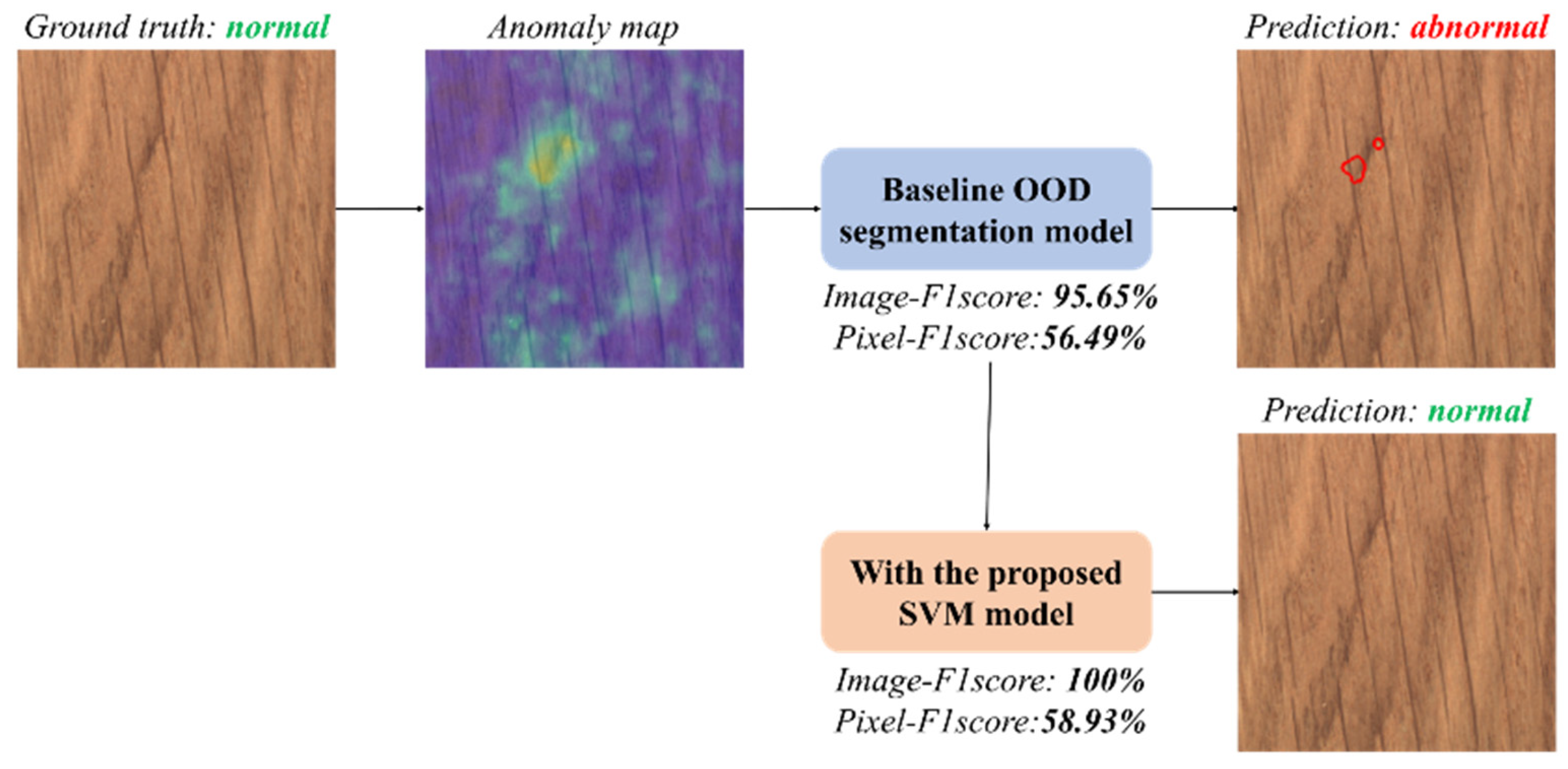
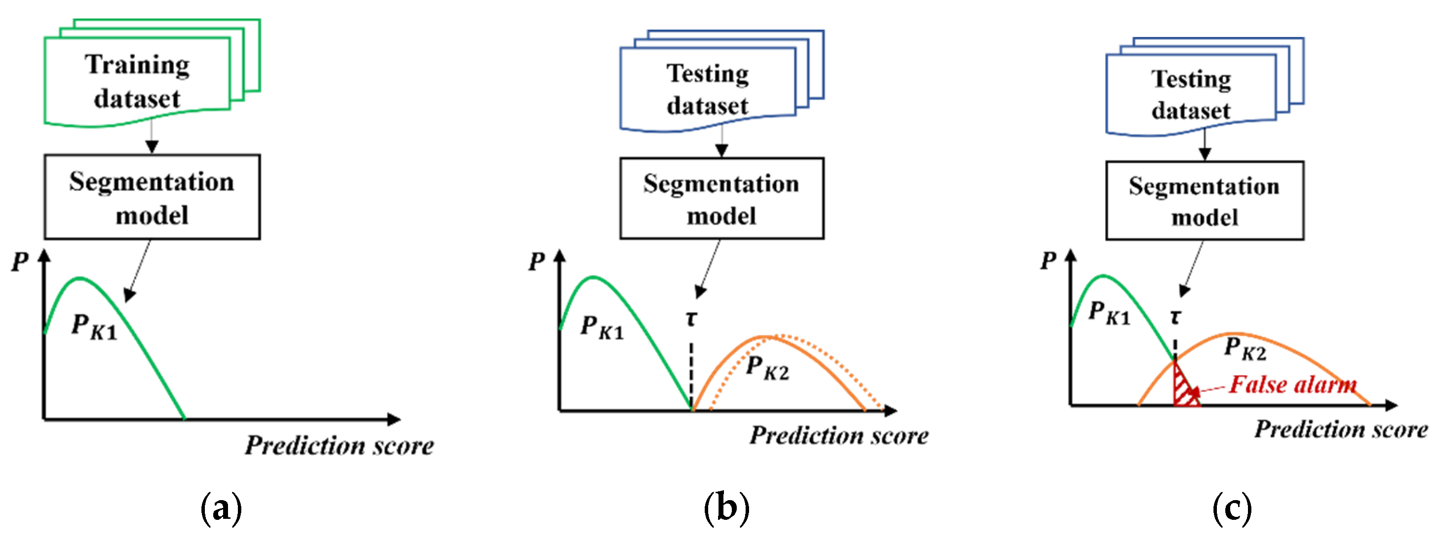
3.1. False Alarm in Unsupervised Anomaly Detection

Unsupervised anomaly detection falls into the OOD domain as detectors learn from the anomaly-free training dataset.
Given an anomaly-free training dataset with D images: χ = x 0 , x 1 , , x D , x i R H × W , the UAD model aims to train a neural network-enabled anomaly score learning function S : χ K that differentiates the anomalies from normal ones. The separation unit is an image, object, or pixel, depending on the granularity of the specific visual task. To investigate the cause of false alarms in OOD defect segmentation tasks, we may have a further statistical analysis of the pixel-wise transformed outputs S χ , which are prediction scores on anomaly maps K , and finally turn into segmentation mask via binary threshold τ . Generally, the score falls in 0 , 1 while a higher value indicates a higher likelihood of belonging to a defect.
The density probability distributions of prediction scores estimated by the OOD segmentation model in each phase are illustrated in Figure 2. During the training phase, depicted in Figure 2a, the model learns the feature distribution of anomaly-free images and trains its parameters to map the original images to the prediction score distribution corresponding to P K 1 . In principle, the mapped anomaly score should be lower than the default threshold, indicating a negative attribute. Figure 2b,c illustrate the segmentation process in ideal and real-world industrial anomaly detection scenarios, respectively. In an ideal scenario, the segmentation model should be capable of mapping normal pixels in the image to prediction scores P K 1 lower than the decision threshold τ , forming negative predictions. At the same time, it should map pixels corresponding to anomalies or faults to anomaly scores higher than the decision threshold, forming positive predictions P K 2 , as shown in Figure 2b, representing a perfect segmentation situation.
The discriminative ability of unsupervised models is challenged as the absence of defects from the training dataset, especially dealing with complex anomaly detection scenarios. In practical applications, anomaly-free images involve various adverse factors causing appearance differences, including lighting conditions, clutter background, product batch, slight in-service aging, and staff stamps. Therefore, the discrimination abilities of unsupervised detectors are usually incompatible with the complex classification boundary between defect and normal. The model may not accurately predict anomalous pixels on the image. Prediction scores for normal and defect pixels intersect, as shown in Figure 2c. When two distributions intersect, the resulting performance will have deficiencies no matter where the threshold τ locates. The binarization of the prediction score using τ results in the formation of false positives, represented by the portion of P K 2 above the threshold τ , which corresponds to false alarms in industrial anomaly detection.
Simply increasing τ to avoid the intersection with P K 1 may eliminate false alarms while causing positive defects to be ignored. Therefore, the false alarm problem comes from the inadequate discrimination ability to differentiate P K 1 and P K 2 . The performance can hardly optimize through existing parameter modification since there is no additional information on defects. To this end, we provide a post-processing optimization approach to incorporate fuzzy domain knowledge of defects to eliminate false alarms at the pixel level.

3.2. Proposed Post-Processing Optimization Method

Figure 3 illustrates our proposed optimization process for OOD segmentation models, in which an SVM classification model is integrated after the baseline defect detection model to filter out false alarms from positive prediction patches.
The detection process of the baseline OOD segmentation model is illustrated in Figure 3 with blue arrows. In this process, the model takes the input image χ and maps it to anomaly maps K , which are then transformed into a segmentation mask using a binary threshold τ .
The proposed method operates on the binary segmentation results during the testing phase, as illustrated by the red arrows. This conceptualization stems from an observation made during our experiments: a trained segmentation model tends to produce false positives exhibiting distribution patterns similar to those of high-score regions when provided with anomaly-free images as inputs. Such a scenario is commonplace in industrial settings, where images often follow specific acquisition patterns. Consequently, different positions in an image hold corresponding real-world significance, potentially aligning with a component of the system under inspection. Thus, we leverage the distribution characteristics of positive patches to eliminate false alarms.
During the testing phase, the baseline OOD model generates a binary candidate mask, where white pixels indicate positives. This candidate mask undergoes connected-component analysis, resulting in multiple subregions, namely positive patches. Bounding boxes are then generated for each patch. Following this, the devised classification model systematically identifies false alarms from these patches based on their distribution characteristics, specifically considering the centroid and scale of each bounding box. Positive patches exhibiting distribution characteristics consistent with those high-score regions in the anomaly maps of anomaly-free images are classified as false positives. Subsequently, their predictions are corrected to negative.
To underscore the effectiveness of post-processing using patch-level features in our work, the selection of the binary classification model primarily hinges on its efficiency rather than complex architecture. This choice is grounded in the recognition that the dimensionality of the input vectors is considerably limited compared to image data. The classification model is a soft-margin SVM model capturing the distribution characteristics of false alarm patches.
Donate the input vector as o n and the label indicating a false alarm or a defect as y n , and thus the distance between the closest sample to the hyperplane is:
m a r g i n w = min n = 1 , , N d i s t a n c e o n , w
Hence, the objective function of the classifier is:
max w m a r g i n w s . t .   y n w T x n > 0
The kernel of feature transformation is the radial basis function, also known as Gaussian kernel, which improves the computation efficiency of this quadratic programming problem. Kernel learning maps the original linear indivisibility distributions into separable higher dimensions with limited computation cost. The original input space consistent with n input samples may turn into the separable feature dimension with a maximum of n dimensions through transformation. Donating the mapping function as ϕ and width of the kernel as σ , the radial basis function is:
K o i , o j = ϕ o i ϕ o j = e x p | o i o j | 2 2 σ 2
During the testing stage, o n is automatically generated from positive patches identified on candidate masks by the segmentation model. The classification model assigns a false alarm probability score to each candidate patch. If the false alarm probability score of a positive patch exceeds the threshold of 0.5, it is classified as a false positive, triggering subsequent post-processing steps at both pixel and image levels.
Pixels associated with this patch undergo multiplication by a coefficient, c p , to attenuate their impact on the anomaly map, thereby aiding in the reduction in false alarms in the segmentation mask. Simultaneously, the image-level prediction score for this image decreases proportionally to the area ratio of this patch relative to the entire image.

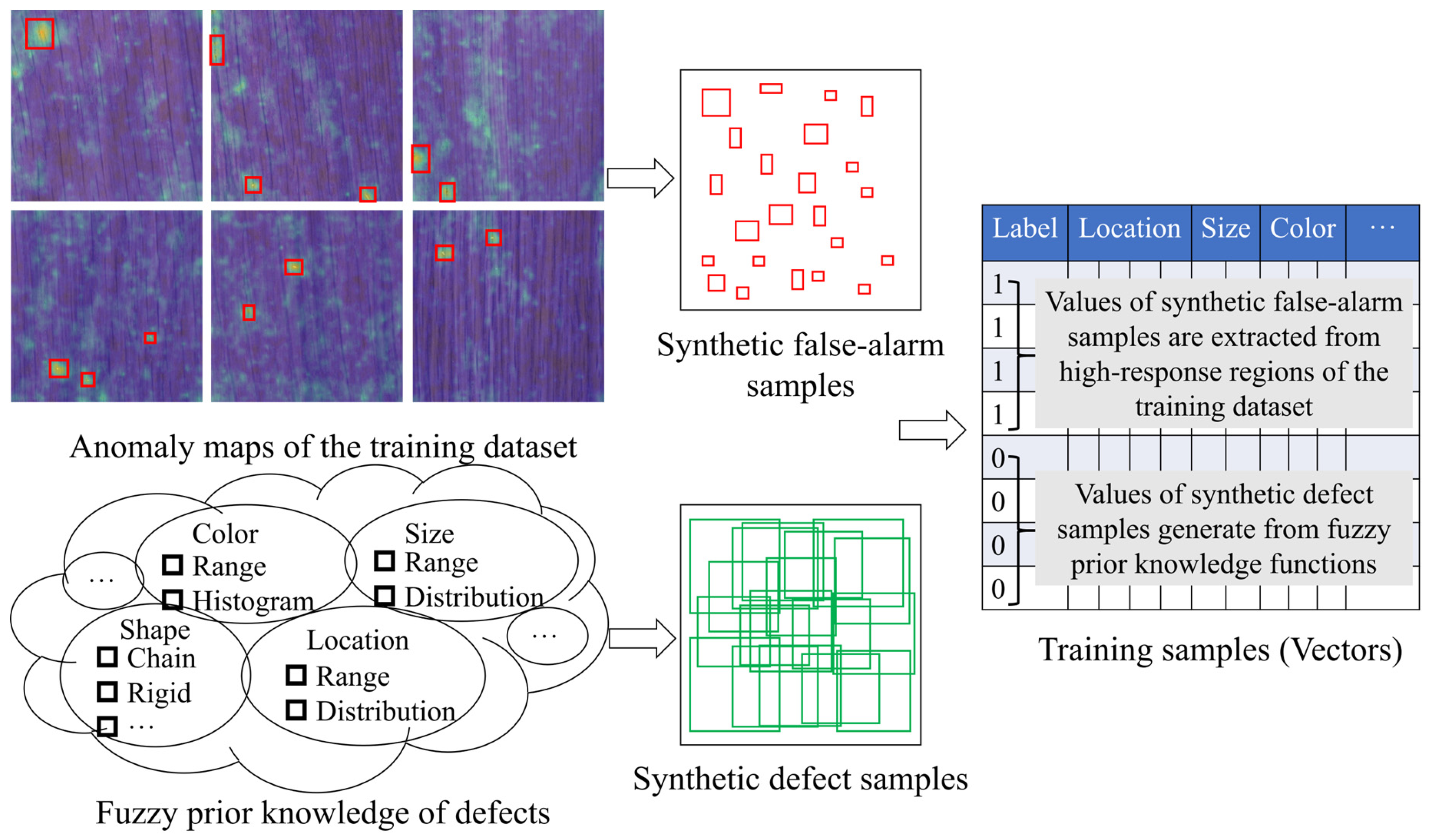
3.3. Unsupervised Sample Synthesis for Classifier Training

One of the challenges posed by our proposed method is the training sources of the classification model. To address this, we devise a sample synthesis strategy that generates training samples tailored to the specific detector and application. Note that the training samples for the classification model are not images but the vectors capturing distribution characteristics of false-positive and true-positive patches.
As previously mentioned, the distribution characteristics, specifically considering the centroid and scale of each bounding box, of false positives in the testing dataset are similar to high-score regions on the anomaly maps of anomaly-free images. This distribution characteristics can be further expanded into other patch-level features, such as color, texture, shape, and other features. The choice of patch-level features dictates the dimensions of our training samples (vectors), determined by the discriminative attributes relevant to the specific application.
As depicted in Figure 4, the training samples (vectors) are consistent with synthetic false alarm samples and synthetic defect samples. The synthetic false alarm samples originate from high-score patches on the anomaly maps of the trained segmentation detector for the anomaly-free training dataset. The synthetic defect samples come from fuzzy domain-specific knowledge.
The synthetic false alarm samples provide insights into the anomaly maps of the training dataset, particularly in regions where their high-score regions are similar to those of false alarm patches. To acquire information regarding false alarms, we closely examine the anomaly maps generated from the training dataset. The anomaly map serves as an intermediate output of pixel-wise predictions and reflects the detector’s estimations of anomaly levels within the input image. Even the anomaly maps of the training samples may manifest high-response regions when the trained detector demonstrates sub-optimal performance in intrinsic industrial scenarios. As pixel-wise predictions are derived from thresholding the anomaly map, regions highlighted in yellow or green in Figure 5 correspond to false alarms. This observation underscores the limited discrimination ability of the detector on the training dataset, leading to false alarms during the testing stage. By treating these high-response patches as synthetic false alarms, we can extract their patch-level features to form synthetic false alarm samples (vectors).
Synthetic defect samples are generated from fuzzy domain knowledge, encompassing intuitive patch-level features such as centroid, size, color, texture, and shape. For instance, when detecting faults related to a specific rigid component, the centroid and scale of the patch occupied by this component, like a common component tend to be relatively stable due to the fixed distance between the capturing camera and the surveillance target in industrial anomaly detection scenarios. In the case of missing faults, the patch corresponding to true defects aligns with the original centroid and scale of the component. For locally damaged faults, the pixels of the corresponding patch represent a subset of the originally occupied area of the component. In the case of foreign object faults, the distribution attributes of the image block can be inferred based on the common types of foreign objects and their typical attachment forms, utilizing latent images of foreign objects to extract shape and texture features.
The fuzzy prior knowledge is derived from the empirical understanding of fault categories in specific industrial settings. It eliminates the requirement for collecting real-world fault images, requiring only empirical and probabilistic summaries to generate synthetic defect samples (vectors). Specifically, the synthetic defect samples are generated by a defect sample generator, which is a random vector generator conforming to specified distributions determined by domain knowledge. The fuzzy prior knowledge guides the distribution type and corresponding parameters of each dimension. For example, the x-coordinate of the centroid of the image block follows a normal distribution with a mean of 100 and a standard deviation of 10, while the height follows a uniform distribution in the range [160, 200].
Patch-level features derived from domain-specific prior knowledge serve as a guiding framework for generating synthetic defect samples, acknowledging potential imprecision in comparison to real-world data. In binary classification models, the inclusion of synthetic false alarm samples plays a crucial role in fortifying the robustness, allowing it to withstand errors in the precision of training defect samples.
Furthermore, the training samples for the SVM classifier need to maintain a balance between the two classes, ensuring a similar quantity of synthetic defect samples and synthetic false alarm samples to avoid overfitting issues on either class. In practice, a common challenge arises from the limited quantity of training images, leading to an insufficient number of synthetic false alarm samples. In such cases, we employ basic augmentation techniques, including noise addition, positional translation, and symmetry adjustments, tailored to the specific requirements of the application.

4. Experiments

In this section, we conduct experiments using two advanced anomaly detection models as baseline models on two industrial applications to evaluate the performance of the proposed post-processing method against the baseline segmentation model. The parameters of baseline segmentation algorithms are constant in comparative experiments.

4.1. Experimental Settings

Experimental settings are delineated in this subsection. In following experiments, the classification is realized by harnessing the joint distribution of bounding box centroid and size. The threshold for the false alarm probability score and the false-positive pixel coefficient c p are set to 0.5; thus, any positive prediction will be negative. The reduction in the image-level prediction score is three times the elimination area ratio to entire image. Furthermore, in the SVM model’s training phase, we adopt a cross-validation methodology with a partition of 70% for training and 30% for validation. This is coupled with a grid search strategy, allowing for a systematic exploration of hyperparameter values to ensure the model’s optimal performance.

4.1.1. Experimental Dataset

Our experiments revolve around two distinct industrial applications: wood defect examination, utilizing the wood category within the MVTec AD dataset [15], and freight train monitoring, employing the TFDS-RP dataset.
The MVTec anomaly detection dataset is a widely recognized and publicly available industrial defect inspection dataset. Within the MVTec AD dataset, the wood category stands out, comprising 247 training images and 79 test images, all with a resolution of 1024 × 1024 pixels. Abnormal images in the testing dataset cover five types of defects: color, hole, liquid, scratch, and combined. These defects manifest as conspicuous alterations in texture, presenting varying sizes.
In contrast, the TFDS-RP dataset introduces a more complex application environment. This dataset consists of authentic images captured during the operation of railway freight trains. These images have been cropped to 128 × 128 pixels, focusing on a specific circular component, namely a brake pad locking ring. The absence or deformation of this component could potentially compromise the safety of the running vehicle, making it a relatively high-frequency fault. The TFDS-RP dataset comprises 387 training images and 100 test images, encompassing two fault types: locking ring deformation and locking ring loss.
Notably, images within the TFDS-RP dataset originate from outdoor settings by trackside cameras. Consequently, these images exhibit a wider range of lighting conditions and positional variations, rendering fine-grained detection significantly more challenging.

4.1.2. Baseline OOD Model

We selected two state-of-the-art defect detection algorithms, Fastflow [14] and Cflow [39], as our baseline models.
Fastflow is a 2D-normalizing flow designed for anomaly detection and localization. It leverages fully convolutional networks and a two-dimensional loss function to effectively model both global and local feature distributions. It is constructed with a lightweight network structure characterized by the alternating stacking of large and small convolution kernels. This design enhances its efficiency and allows for end-to-end inference. FastFlow is adaptable and can function as a plugin model with various feature extractors. In the following experiment, we retain the original design that uses the features of the last layer in the first three blocks and put these features into the 2D flow model to obtain their respective anomaly detection and localization results. The training process involves an Adam optimizer with a learning rate of 1 × 10⁻³, weight decay of 1× 10⁻⁵, 500 epochs, and a batch size of 32.
Cflow is based on conditional normalizing flows and shares similarities with CNNs in terms of feature map spatial dimensions. This similarity results in higher accuracy metrics and lower computational and memory requirements. The main idea behind CFLOW-AD is to learn the distribution of anomaly-free image patches and transform it into a Gaussian distribution. This transformation allows the model to separate in-distribution patches from out-of-distribution patches using a threshold. The training hyperparameters for CFLOW-AD include the use of the Adam optimizer with a learning rate of 1 × 10⁻⁴, 100 training epochs, and a mini-batch size of 32 for the encoder. Cosine learning rate annealing is applied with two warm-up epochs. The CFLOW-AD decoders are unable to feature map dimensions and have low memory requirements. Both training and testing phases involve the sampling of feature vectors.
Their source codes are publicly available. Experimental settings in the following sections are given in Table 1. We compare their performance with revised models that incorporate our proposed post-processing model.

4.1.3. Performance Evaluation

To achieve comprehensive assessments, we exploit the pixel-wise output of these algorithms and make comparisons with baseline algorithms using four metrics: image-level AUROC (area under the receiver operating characteristic), image-level F1-score, pixel-level AUROC, and pixel-level F1-score. All the performance metrics are evaluated based on the confusion matrix, which consists of four classes: true positive (TP), false positive (FP), false negative (FN), and true positive (TP). Note that the positive samples in the defect inspection task refer to images with defect regions or pixels in a defect area.
The AUROC is calculated as the area under the ROC curve. A ROC curve shows the trade-off between the true positive rate and false positive rate across different decision thresholds. For the following unsupervised binary image-wise or pixel-wise classification tasks, AUROC is more informative in telling the discrimination ability of the model considering the potential data imbalance, especially from the pixel level.
Moreover, F1-score leverages precision and recall into a single measure that captures both properties. The calculation process of the F1-score is obtained through Equations (4)–(6).
p r e c i s i o n = T P T P + F P × 100 %
r e c a l l = T P T P + F N × 100 %
F 1 - s c o r e = 2 × p r e c i s i o n × r e c a l l p r e c i s i o n + r e c a l l × 100 %

4.2. Quantitative Experimental Results

Our quantitative results, as presented in Table 2 and Table 3, provide comparisons of AUROC and F1-scores at both the image and pixel levels. These results confirm significant improvements over baseline algorithms.
On the MVTec-wood dataset, both baseline models achieve perfect image-level AUROC scores. This implies that, under reasonable image-level thresholds, they can correctly classify all images. However, from an image-level perspective, their predictions exhibit bias due to the default 0.5 threshold. According to the image-level post-processing strategy for determined false alarms, the filtered predictions of both trackers achieve perfect predictions for the two image-level metrics. Pixel-level metrics also validate the effectiveness of this paper’s approach. Specifically, the two metrics for Fastflow improve by 1.34% and 4.32%, respectively, compared to the unfiltered results. For Cflow, the corresponding improvements are 1.25% and 6.83%.
The TFDS-RP dataset also validates the effectiveness of the proposed method in removing false alarms and improving overall performance. Given the higher complexity of this scenario, baseline predictions perform inferiorly compared to the wood examination application. None of the methods achieve correct image-level predictions. Specifically, Fastflow’s image-level F1-score is improved by 40% through our method, as it correctly eliminates 24 image-level false positives. For Cflow, our method improves the image-level F1-score by 69.58%, as it correctly eliminates 16 image-level false positives. Despite the challenging lighting and complex background in this scenario, this paper’s method still makes significant progress in pixel-level metrics.

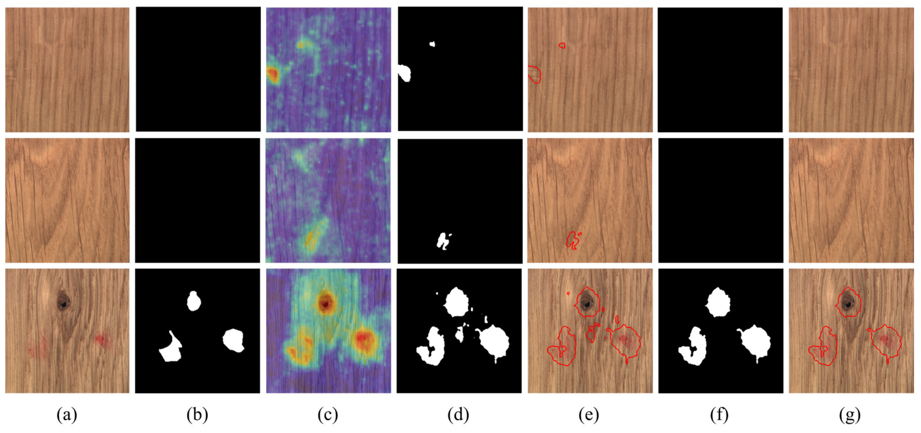
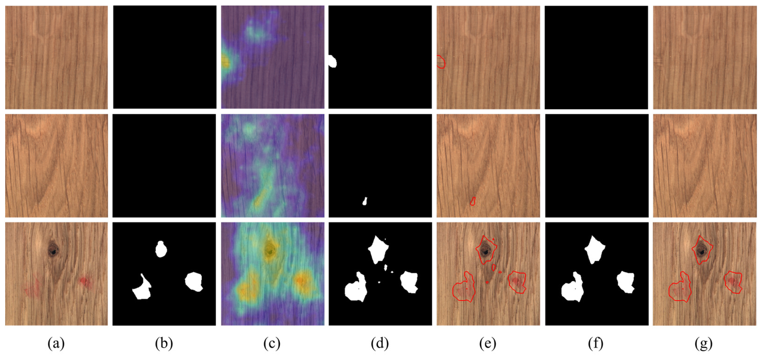
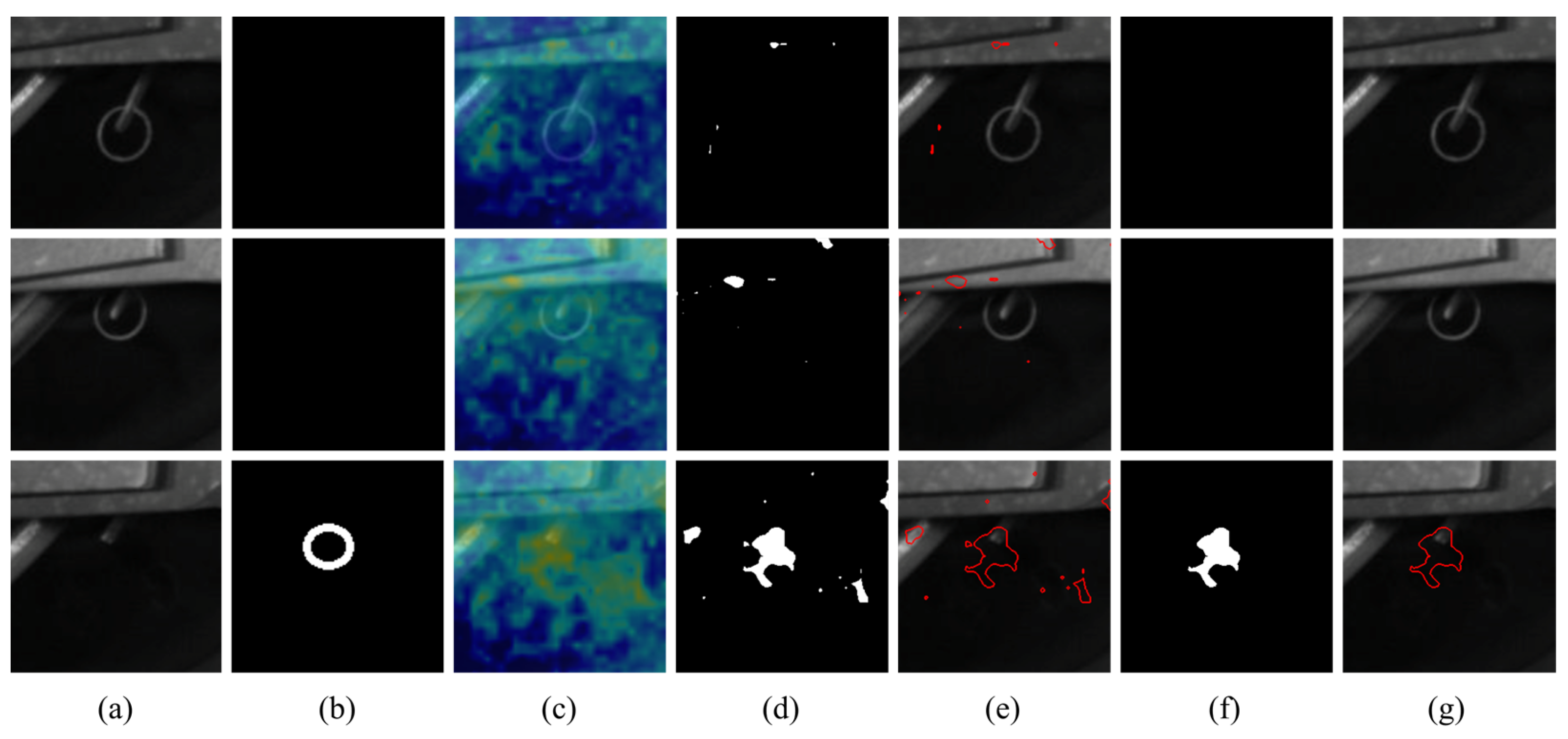
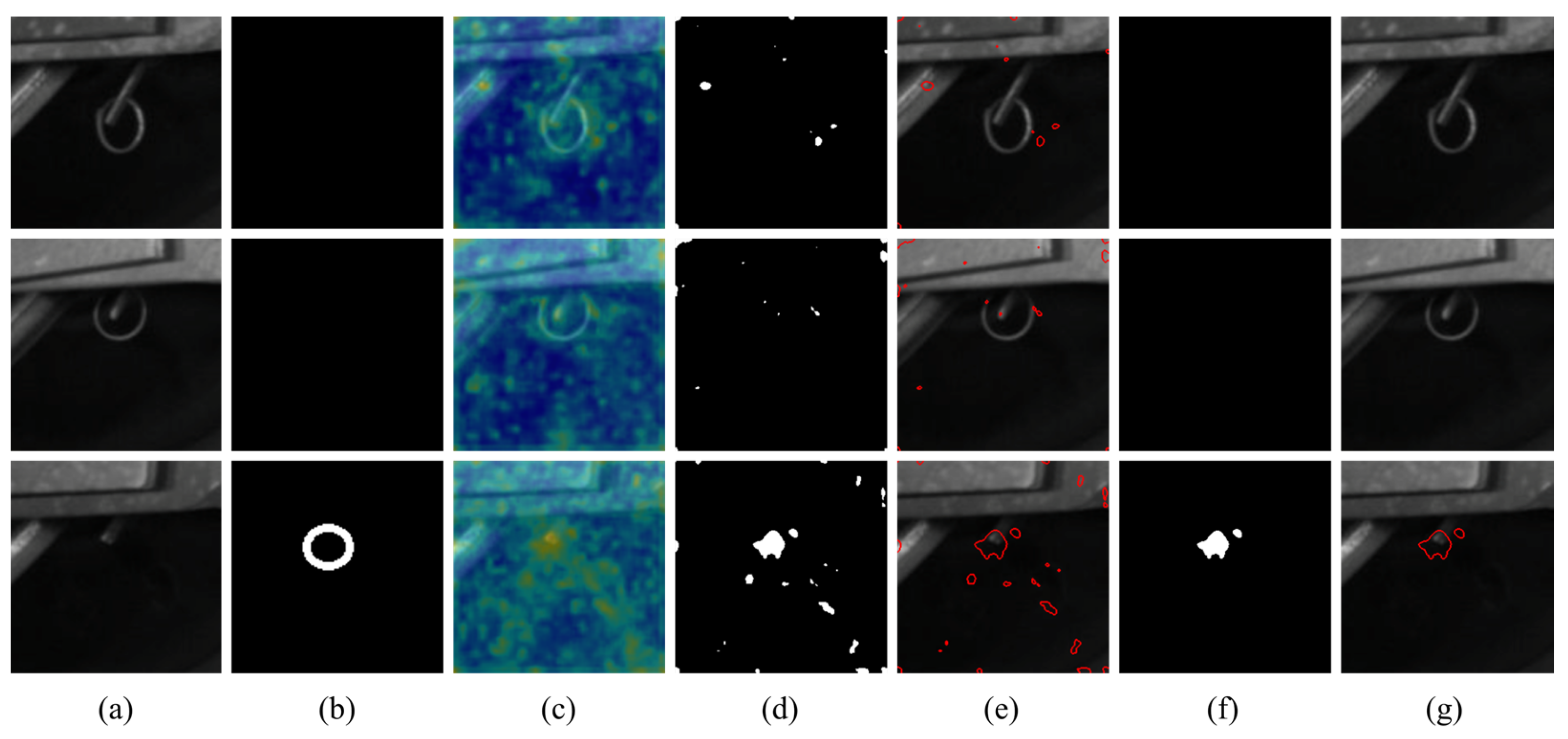
4.3. Visual Comparisons for Pixel-Wise Segmentation

As depicted in Figure 6, Figure 7, Figure 8 and Figure 9, the top two rows illustrate false alarms on anomaly-free images, and our proposed method effectively identifies and eliminates false alarm pixels. Despite the heterogeneity in the distribution of false alarms, our proposed method adaptively enhances the results. The bottom rows in these figures showcase defects in the test images after filtering, highlighting the discrimination capability of the post-processing model.
Figure 6, Figure 7, Figure 8 and Figure 9 provide intuitive examples of the impact of our method on two OOD models. These examples validate the points made in this paper, thoroughly confirming the effectiveness of the proposed approach. Since this paper primarily addresses the issue of false alarms in industrial anomaly detection, and the occurrence probability of anomalies themselves is exceedingly low, we have selected two examples from each experimental result: one showcasing the effects on anomaly-free images (negative) and one displaying the detection performance on a defect (positive) test image.
Specifically, in the first and second rows of Figure 6, the baseline FastFlow generates false alarms in the form of small blocks during prediction. These false alarms are successfully filtered out by our method. In the third row, which presents a combined defect image containing three abnormal regions, the baseline generates more predictions, many of which are disconnected small pixel blocks. It is evident that our method eliminates these small false positives while preserving true positive predictions, with no impact on the recall rate.
Similarly, Figure 7 illustrates the performance of Cflow on these three images. The false alarms generated by Cflow exhibit some similarity to those of Fastflow. One possible explanation is that both models employ feature extraction networks trained on large-scale models, possibly leading to strong responses to pixel changes in the corresponding regions of the image. As this phenomenon exists in both the training and test sets, our method effectively captures and eliminates this type of false alarm.
As indicated by the performance metrics in Table 3, false alarms are quite frequent in the TFDS-RP dataset, especially at the object level. In Figure 8, FastFlow generates numerous small predictions on defect-free images. These false alarms may be attributed to the complexity of the scene. In this scenario, pixel variations in some local regions may be caused by factors such as lighting differences, component aging, and complex backgrounds. However, FastFlow captures these drastic changes in adjacent pixels and predicts them as positive. In reality, these false positives are also abundant in the anomaly maps of the training set. Consequently, our method effectively captures and filters out this model and, as seen in the third row depicting images of pinhole loss defects, successfully eliminates false alarms, preserving regions corresponding to actual fault areas. It is worth noting that the annotation strategy used for the TFDS-RP dataset is the same as that of the MVTec dataset, which labels pixels that may differ from the normal state as anomalies. This labeling method may lead to low F1-score results for both methods, even if the predicted regions are approximately correct at the pixel level. This is a crucial reason for the low F1-score scores for both methods on this dataset.
Cflow’s performance in Figure 9 is similar, with Cflow’s false alarm regions being slightly larger compared to those of Fastflow. From the last two columns, it is evident that our method successfully removes most false positives in the example images. The preserved pixel blocks can provide location information about the fault areas to some extent.

4.4. Parameter Study on Proposed Augmentation Strategy

To further analyze the impact of augmentation methods on virtual samples in practical experiments, we executed a parameter study employing three distinct augmentation settings as depicted in Table 4. The comparative performance evaluation was conducted on the Cflow model using the TFDS-RP dataset. The three augmentation settings are delineated as follows:
Setting #1: Utilizing only synthesized false alarm samples generated from the anomaly maps of the anomaly-free training dataset at three binary thresholds [0.4, 0.45, 0.5].
Setting #2: Utilizing only synthesized false alarm samples generated from the anomaly maps of the anomaly-free training dataset at seven binary thresholds [0.4, 0.41, 0.42, 0.43, 0.44, 0.45, 0.5].
Setting #3: Employing synthesized false alarm samples generated from the anomaly maps of the anomaly-free training dataset at three binary thresholds [0.4, 0.45, 0.5] with additional Gaussian noise as augmentation.
Observations reveal that both Setting #2 and Setting #3 achieved notable improvements in detection results, effectively eliminating image-level false positives compared to Setting #1. This success can be attributed to the utilization of object-level semantic features in our method. Moreover, Setting #2 and Setting #3 achieve identical performance metrics, that is, the increment in threshold numbers or additional augmentation strategies may lead to stable filtering performance when the classifier’s training samples are sufficiently abundant.
Furthermore, all three settings exhibited significant enhancements compared to baseline performances, reaffirming the efficacy of our proposed method.
This comprehensive parameter analysis elucidates the performance variations across different augmentation settings, substantiating the robustness and effectiveness of our proposed synthesized strategy.

5. Conclusions

In this article, we introduce a novel approach to tackle the challenges faced by OOD segmentation algorithms in industrial anomaly detection. Our method revolves around a post-processing module, meticulously designed to discern intricate distinctions between false alarms and genuine defects within specific industrial applications.
Furthermore, we present an innovative false alarm sampling strategy for OOD segmentation models. This strategy empowers us to generate essential training samples without additional labeled images.
Our experimental results are comprehensive, entailing the evaluation of two advanced unsupervised anomaly detection algorithms, Cflow and FastFlow, across two distinct industrial applications. We also provide a parameter analysis experiment, shedding light on the augmentation settings employed on the two datasets. The results from these experiments unequivocally affirm the efficacy of the proposed method.
The proposed method is founded on the presumption of analogous patch-level false alarm patterns between the training and testing datasets. Consequently, its applicability is constrained by the specificity of this characteristic.
By addressing the challenges in industrial anomaly detection, our work contributes to the efficient false alarm elimination of unsupervised deep learning models. Our work specifically focuses on providing practical enhancements to anomaly detection tailored for industrial applications, leveraging the nuances of fuzzy domain knowledge. Future endeavors will extend to exploring false alarm elimination across a broader spectrum of state-of-the-art methods. We aim to delve into the underlying causes of high activations on anomaly maps, seeking a deeper understanding. Additionally, we will strive to enhance detection performance without relying on knowledge beyond the anomaly-free training dataset.

Author Contributions

J.Q.: conceptualization, methodology, software, validation, analysis, writing; H.S.: methodology, resources, analysis, writing, funding acquisition; Y.H.: conceptualization, methodology, analysis, validation; Z.Y.: methodology, supervision, funding acquisition. All authors have read and agreed to the published version of the manuscript.

Funding

This work was supported by the Fundamental Research Funds for the Central Universities (Science and technology leading talent team project 2022JBXT005), the State Key Laboratory of Advanced Rail Autonomous Operation (Contract No. RAO2023ZZ003), and the Technology Development Program of China Energy Investment Corporation (Grant GJNY-21-65 and Grant GJNY-20-139).

Institutional Review Board Statement

Not applicable.

Informed Consent Statement

Not applicable.

Data Availability Statement

Data are contained within the article.

Conflicts of Interest

The authors declare no conflict of interest.

References

  1. Sharma, M.; Lim, J.; Lee, H. The Amalgamation of the Object Detection and Semantic Segmentation for Steel Surface Defect Detection. Appl. Sci. 2022, 12, 6004. [Google Scholar] [CrossRef]
  2. Luo, H.; Cai, L.; Li, C. Rail Surface Defect Detection Based on An Improved YOLOv5s. Appl. Sci. 2023, 13, 7330. [Google Scholar] [CrossRef]
  3. Kang, G.; Gao, S.; Yu, L.; Zhang, D. Deep Architecture for High-Speed Railway Insulator Surface Defect Detection: Denoising Autoencoder with Multitask Learning. IEEE Trans. Instrum. Meas. 2019, 68, 2679–2690. [Google Scholar] [CrossRef]
  4. Liu, Y.; Garg, S.; Nie, J.; Zhang, Y.; Xiong, Z.; Kang, J.; Hossain, M.S. Deep Anomaly Detection for Time-Series Data in Industrial IoT: A Communication-Efficient On-Device Federated Learning Approach. IEEE Internet Things J. 2021, 8, 6348–6358. [Google Scholar] [CrossRef]
  5. Thombre, S.; Zhao, Z.; Ramm-Schmidt, H.; Garcia, J.M.V.; Malkamaki, T.; Nikolskiy, S.; Hammarberg, T.; Nuortie, H.; Bhuiyan, M.Z.H.; Sarkka, S.; et al. Sensors and AI Techniques for Situational Awareness in Autonomous Ships: A Review. IEEE Trans. Intell. Transp. Syst. 2022, 23, 64–83. [Google Scholar] [CrossRef]
  6. Jezequel, L.; Vu, N.-S.; Beaudet, J.; Histace, A. Efficient Anomaly Detection Using Self-Supervised Multi-Cue Tasks. IEEE Trans. Image Process. 2023, 32, 807–821. [Google Scholar] [CrossRef] [PubMed]
  7. Doorenbos, L.; Sznitman, R.; Márquez-Neila, P. Data invariants to understand unsupervised out-of-distribution detection. In Computer Vision—ECCV 2022; Part XXXI; Lecture Notes in Computer Science; Springer: Berlin/Heidelberg, Germany, 2022; Volume 13691, pp. 133–150. [Google Scholar]
  8. Ran, X.; Xu, M.; Mei, L.; Xu, Q.; Liu, Q. Detecting out-of-distribution samples via variational auto-encoder with reliable uncertainty estimation. Neural Netw. 2022, 145, 199–208. [Google Scholar] [CrossRef] [PubMed]
  9. Ruff, L.; Kauffmann, J.R.; Vandermeulen, R.A.; Montavon, G.; Samek, W.; Kloft, M.; Dietterich, T.G.; Muller, K.-R. A Unifying Review of Deep and Shallow Anomaly Detection. Proc. IEEE 2021, 109, 756–795. [Google Scholar] [CrossRef]
  10. Saha, S.; Bovolo, F.; Bruzzone, L. Change Detection in Image Time-Series Using Unsupervised LSTM. IEEE Geosci. Remote. Sens. Lett. 2022, 19, 1–5. [Google Scholar] [CrossRef]
  11. Zhang, Y.; Chen, Y.; Wang, J.; Pan, Z. Unsupervised Deep Anomaly Detection for Multi-Sensor Time-Series Signals. IEEE Trans. Knowl. Data Eng. 2023, 35, 2118–2132. [Google Scholar] [CrossRef]
  12. Rao, W.; Qu, Y.; Gao, L.; Sun, X.; Wu, Y.; Zhang, B. Transferable network with Siamese architecture for anomaly detection in hyperspectral images. Int. J. Appl. Earth Obs. Geoinf. 2022, 106, 102669. [Google Scholar] [CrossRef]
  13. Wang, H.; Zhang, A.; Zhu, Y.; Zheng, S.; Li, M.; Smola, A.J.; Wang, Z. Partial and Asymmetric Contrastive Learning for Out-Of-Distribution Detection in Long-Tailed Recognition. In Proceedings of the 39th International Conference on Machine Learning, Baltimore, MD, USA, 17–23 July 2022. [Google Scholar]
  14. Yu, J.; Zheng, Y.; Wang, X.; Li, W.; Wu, Y.; Zhao, R.; Wu, L. Fastflow: Unsupervised anomaly detection and localization via 2d normalizing flows. arXiv 2021, arXiv:2111.07677. [Google Scholar]
  15. Drost, B.; Ulrich, M.; Bergmann, P.; Hartinger, P.; Steger, C. Introducing mvtec—A dataset for 3d object recognition in industry. In Proceedings of the IEEE International Conference on Computer Vision Workshops, Venice, Italy, 22–29 October 2017; pp. 2200–2208. [Google Scholar]
  16. Jiang, J.; Zhu, J.; Bilal, M.; Cui, Y.; Kumar, N.; Dou, R.; Su, F.; Xu, X. Masked Swin Transformer Unet for Industrial Anomaly Detection. IEEE Trans. Ind. Inform. 2023, 19, 2200–2209. [Google Scholar] [CrossRef]
  17. Alvarenga, W.J.; Campos, F.V.; Costa, A.C.; Salis, T.T.; Magalhães, E.; Torres, L.C.; Braga, A.P. Time domain graph-based anomaly detection approach applied to a real industrial problem. Comput. Ind. 2022, 142, 103714. [Google Scholar] [CrossRef]
  18. Kong, F.; Li, J.; Jiang, B.; Wang, H.; Song, H. Integrated generative model for industrial anomaly detection via bidirectional lstm and attention mechanism. IEEE Trans. Ind. Inform. 2023, 19, 541–550. [Google Scholar] [CrossRef]
  19. Zayas-Gato, F.; Jove, E.; Casteleiro-Roca, J.; Quintián, H.; Piñón-Pazos, A.; Simić, D.; Calvo-Rolle, J.L. A hybrid one-class approach for detecting anomalies in industrial systems. Expert Syst. 2022, 39, e12990. [Google Scholar] [CrossRef]
  20. Zeiser, A.; Özcan, B.; van Stein, B.; Bäck, T. Evaluation of deep unsupervised anomaly detection methods with a data-centric approach for on-line inspection. Comput. Ind. 2023, 146, 103852. [Google Scholar] [CrossRef]
  21. Yu, L.; Wang, Y.; Zhou, L.; Wu, J.; Wang, Z. Residual neural network-assisted one-class classification algorithm for melanoma recognition with imbalanced data. Comput. Intell. 2023, 1–18. [Google Scholar] [CrossRef]
  22. Han, P.; Li, H.; Xue, G.; Zhang, C. Distributed system anomaly detection using deep learning-based log analysis. Comput. Intell. 2023, 39, 433–455. [Google Scholar] [CrossRef]
  23. Kerboua, A.; Kelaiaia, R. Fault Diagnosis in an Asynchronous Motor Using Three-Dimensional Convolutional Neural Network. Arab. J. Sci. Eng. 2023, 1–19. [Google Scholar] [CrossRef]
  24. Tran, T.M.; Vu, T.N.; Vo, N.D.; Nguyen, T.V.; Nguyen, K. Anomaly Analysis in Images and Videos: A Comprehensive Review. ACM Comput. Surv. 2023, 55, 1–37. [Google Scholar] [CrossRef]
  25. Shen, H.; Wei, B.; Ma, Y.; Gu, X. Unsupervised industrial image ensemble anomaly detection based on object pseudo-anomaly generation and normal image feature combination enhancement. Comput. Ind. Eng. 2023, 182, 109337. [Google Scholar] [CrossRef]
  26. Liu, K.; Chen, B.M. Industrial uav-based unsupervised domain adaptive crack recognitions: From database towards real-site infrastructural in-spections. IEEE Trans. Ind. Electron. 2023, 70, 9410–9420. [Google Scholar] [CrossRef]
  27. Tong, G.; Li, Q.; Song, Y. Two-stage reverse knowledge distillation incorporated and Self-Supervised Masking strategy for industrial anomaly detection. Knowl. Based Syst. 2023, 273, 110611. [Google Scholar] [CrossRef]
  28. Park, J.-H.; Kim, Y.-S.; Seo, H.; Cho, Y.-J. Analysis of training deep learning models for pcb defect detection. Sensors 2023, 23, 2766. [Google Scholar] [CrossRef] [PubMed]
  29. de Oliveira, D.C.; Nassu, B.T.; Wehrmeister, M.A. Image-based detection of modifications in assembled pcbs with deep convolutional autoencoders. Sensors 2023, 23, 1353. [Google Scholar] [CrossRef]
  30. Smith, A.D.; Du, S.; Kurien, A. Vision transformers for anomaly detection and localisation in leather surface defect classification based on low-resolution images and a small dataset. Appl. Sci. 2023, 13, 8716. [Google Scholar] [CrossRef]
  31. Kwon, J.; Kim, G. Distilling distribution knowledge in normalizing flow. IEICE Trans. Inf. Syst. 2023, 106, 1287–1291. [Google Scholar] [CrossRef]
  32. Lo, S.-Y.; Oza, P.; Patel, V.M.M. Adversarially robust one-class novelty detection. IEEE Trans. Pattern Anal. Mach. Intell. 2023, 45, 4167–4179. [Google Scholar] [CrossRef]
  33. Gyimah, N.K.; Gupta, K.D.; Nabil, M.; Yan, X.; Girma, A.; Homaifar, A.; Opoku, D. A discriminative deeplab model (ddlm) for surface anomaly detection and localization. In Proceedings of the IEEE 13th Annual Computing and Communication Workshop and Conference, Las Vegas, NV, USA, 8–11 March 2023; pp. 1137–1144. [Google Scholar]
  34. Rakhmonov, A.A.U.; Subramanian, B.; Olimov, B.; Kim, J. Extensive knowledge distillation model: An end-to-end effective anomaly detection model for real-time industrial applications. IEEE Access 2023, 11, 69750–69761. [Google Scholar] [CrossRef]
  35. Rudolph, M.; Wehrbein, T.; Rosenhahn, B.; Wandt, B. Asymmetric student-teacher networks for industrial anomaly detection. In Proceedings of the IEEE/CVF Winter Conference on Applications of Computer Vision, Waikoloa, HI, USA, 3–7 January 2023; pp. 2591–2601. [Google Scholar]
  36. Hermann, M.; Umlauf, G.; Goldlücke, B.; Franz, M.O. Fast and efficient image novelty detection based on mean-shifts. Sensors 2022, 22, 7674. [Google Scholar] [CrossRef] [PubMed]
  37. Avola, D.; Cascio, M.; Cinque, L.; Fagioli, A.; Foresti, G.L.; Marini, M.R.; Rossi, F. Real-time deep learning method for automated detection and localization of structural defects in manufactured products. Comput. Ind. Eng. 2022, 172, 108512. [Google Scholar] [CrossRef]
  38. Szarski, M.; Chauhan, S. An unsupervised defect detection model for a dry carbon fiber textile. J. Intell. Manuf. 2022, 33, 2075–2092. [Google Scholar] [CrossRef]
  39. Gudovskiy, D.; Ishizaka, S.; Kozuka, K. Cflow-ad: Real-time unsupervised anomaly detection with localization via conditional normalizing flows. In Proceedings of the IEEE Winter Conference on Applications of Computer Vision, Waikoloa, HI, USA, 3–8 January 2022; pp. 1819–1828. [Google Scholar]
  40. Rudolph, M.; Wandt, B.; Rosenhahn, B. Same same but differnet: Semi-supervised defect detection with normalizing flows. In Proceedings of the IEEE Winter Conference on Applications of Computer Vision, Waikoloa, HI, USA, 3–8 January 2021; pp. 1906–1915. [Google Scholar]
  41. Rudolph, M.; Wehrbein, T.; Rosenhahn, B.; Wandt, B. Fully convolutional cross-scale-flows for image-based defect detection. In Proceedings of the IEEE Winter Conference on Applications of Computer Vision, Waikoloa, HI, USA, 4–8 January 2022; Volume 5, pp. 829–1838. [Google Scholar]
Figure 1. Detection results of an OOD model without and with the proposed false-positive classifier on a wood defect detection task. The baseline segmentation model is Fastflow [14], consisting of a deep feature extraction backbone initialized with the ImageNet pre-trained weights and a normalizing flow network trained by the anomaly-free wood images. Parameters of baseline segmentation models freeze during the testing process.
Applsci 13 12655 g001
Figure 2. Density probability distributions of prediction scores. (a) depicts the distribution of anomaly-free targets P K 1 produced by the segmentation model in the training process. (b) shows the ideal condition of OOD models: When the distribution of the anomalies P K 2 is shown as a solid orange line, one threshold exists for successful detection with a perfect AUROC score. Similarly, more thresholds exist for distant distributions like the dotted orange line. (c) presents an actual condition that distributions intersect due to inferior discrimination ability. False alarms arise and are present in the red region.
Applsci 13 12655 g002
Figure 3. The proposed optimization workflow. Blue arrows describe the baseline defect detection processes that directly generate outputs from the baseline segmentation model. Orange arrows present workflows of the devised post-processing method, which filters out false alarms from candidate positive patches. Green arrows draw the sample synthesis and model training process of the SVM classification model depicted in Section 3.3.
Applsci 13 12655 g003
Figure 4. Sample synthesis workflow. Training samples for the classifier are represented as vectors, with their dimensions tailored to the selected discriminative prior knowledge descriptions. Synthetic defect samples are generated based on fuzzy knowledge, while synthetic false alarm samples are derived from high-response regions within the anomaly-free training dataset.
Applsci 13 12655 g004
Figure 5. Anomaly maps of anomaly-free images within a training dataset.
Applsci 13 12655 g005
Figure 6. Visualization of comparative experiments on wood defect examination using Fastflow. Columns correspond to: (a) the test image, (b) ground truth, (c) anomaly map from the baseline OOD model, (d) baseline defect mask, (e) baseline segmentation result, (f) filtered mask, and (g) filtered segmentation result.
Applsci 13 12655 g006
Figure 7. Visualization of comparison experiments on wood defect examination using Cflow. Columns correspond to: (a) the test image, (b) ground truth, (c) anomaly map from the baseline OOD model, (d) baseline defect mask, (e) baseline segmentation result, (f) filtered mask, and (g) filtered segmentation result.
Applsci 13 12655 g007
Figure 8. Visualization of comparison experiments on the round pin examination of a freight train using Fastflow. Columns correspond to: (a) the test image, (b) ground truth, (c) anomaly map from the baseline OOD model, (d) baseline defect mask, (e) baseline segmentation result, (f) filtered mask, and (g) filtered segmentation result.
Applsci 13 12655 g008
Figure 9. Visualization of comparison experiments on a round pin examination of a freight train using Cflow. Columns correspond to: (a) the test image, (b) ground truth, (c) anomaly map from the baseline OOD model, (d) baseline defect mask, (e) baseline segmentation result, (f) filtered mask, and (g) filtered segmentation result.
Applsci 13 12655 g009
Table 1. Experimental settings of the baseline OOD models.
ModelBackbonePretrainedDecoderFlow StepsLearning RateBatchImage Size
FastflowResnet18True-80.00132256
CflowWide_resnet50_2Truefreia-cflow-0.000132256
Table 2. Quantitative performances on MVTec-wood dataset.
ModelImage-Level MetricsPixel-Level Metrics
AUROCF1-ScoreAUROCF1-Score
Fastflow100.00%95.65%96.98%56.49%
Filtered Fastflow100.00%100.00%98.28%58.93%
Cflow100.00%91.67%97.41%58.11%
Filtered Cflow100.00%100.00%98.63%62.08%
Table 3. Quantitative performances on TFDS-RP dataset.
ModelImage-Level MetricsPixel-Level Metrics
AUROCF1-ScoreAUROCF1-Score
Fastflow72.36%28.57%91.13%7.85%
Filtered Fastflow94.74%40.00%91.36%15.24%
Cflow65.78%46.15%88.64%6.84%
Filtered Cflow81.05%78.26%93.58%13.39%
Table 4. Parameter analysis for settings of augmentation strategy.
SettingsImage-Level MetricsPixel-Level Metrics
AUROCF1-ScoreAUROCF1-Score
Cflow65.78%46.15%88.64%6.84%
Filtered Cflow #180.26%75.00%93.41%13.32%
Filtered Cflow #281.05%78.26%93.58%13.39%
Filtered Cflow #381.05%78.26%93.58%13.39%
Disclaimer/Publisher’s Note: The statements, opinions and data contained in all publications are solely those of the individual author(s) and contributor(s) and not of MDPI and/or the editor(s). MDPI and/or the editor(s) disclaim responsibility for any injury to people or property resulting from any ideas, methods, instructions or products referred to in the content.

