Article

Optimization of Data-Driven Soil Temperature Forecast—The First Model in Bangladesh

by
Lipon Chandra Das
1,2,
Zhihua Zhang
1,* and
M. James C. Crabbe
3
1
School of Mathematics, Shandong University, Jinan 250100, China
2
Department of Mathematics, University of Chittagong, Chittagong 4331, Bangladesh
3
Wolfson College, Oxford University, Oxford OX1 1NQ, UK
*
Author to whom correspondence should be addressed.
Appl. Sci. 2023, 13(23), 12616; https://doi.org/10.3390/app132312616
Submission received: 20 October 2023 / Revised: 20 November 2023 / Accepted: 21 November 2023 / Published: 23 November 2023
(This article belongs to the Section Earth Sciences)

Abstract

:
Soil temperature patterns are of great importance for any agro-based economy like Bangladesh since they significantly affect biological, chemical, and physical processes that take place in the soil. Unfortunately, there have been no forecast studies on soil temperature in Bangladesh until now. In this article, we used five tree-based models (decision tree, random forest, gradient boosting tree, a hybrid of decision tree and gradient boosting tree, and a hybrid of random forest and gradient boosting tree) to mine strong links among different meteorological factors and soil temperature at different time window sizes. We found that a hybrid of random forest and gradient boosting tree with all the meteorological factors and a five-day time window is optimal for forecasting soil temperature at depths of 10 cm and 30 cm for all lead times (one, three, or five days), whereas the random forest with the same input scenario and time window is optimal for forecasting soil temperature at a depth of 50 cm for long lead times (five days). Since our study includes the first soil temperature forecast model in Bangladesh, it provides valuable insights for agricultural soil management, fertilizer application, and water resource optimization in Bangladesh, as well as in other South Asian countries that share the same climate patterns as Bangladesh.

1. Introduction

Soil temperature influences the physical, chemical, and microbiological processes that take place in soil [1,2]. It significantly influences the operational seasons of water systems and exerts a profound impact on evapotranspiration, plant growth, development, oxygen availability, and health and yield of various grain crops [3,4,5,6]. A further increase in soil temperature in tropical regions would lead to more negative effects, including seedling death, smaller plants, higher water needs, and increased vulnerability to different plant diseases [7]. At the same time, since soil temperature records can be used to investigate the link between meteorological factors [8], soil temperature often plays a crucial role in numerical weather prediction and is a crucial indicator of climate change patterns [9,10,11,12]. Therefore, monitoring and predicting soil temperature can greatly support the development of sustainable agriculture by providing insights into soil health for seed germination, fruiting, flowering, and the growth of crop species.
Numerous scientific and technical fields have taken notice of the increasing use of machine learning [13,14], largely because of their superior accuracy to conventional forecast techniques and their effectiveness in cutting down on processing time [15,16]. The main advantage of machine learning models is that they are driven by unknown internal links embedded inside data, rather than necessarily taking into account complex physical mechanisms [17]. Schmidt et al. [18] investigated the predictive accuracy and usability of machine learning models in hydrological inference and revealed that machine learning models have high prediction accuracy but relatively low interpretability of inner mechanisms. Although machine learning excels in accuracy and efficiency, it is often opaque and lacks the transparency found in physics-based models. Okkan et al. [19] combined process-oriented, physics-based modeling with machine learning to enhance streamflow estimations and understand the inner mechanisms. Di Salvo [13] used a similar approach to improve existing groundwater numerical modeling. Compared with the process-oriented, physics-based model approach, machine learning can only provide limited insight into understanding soil dynamic changes, but due to the lack of observed data to drive process-oriented, physics-based models in poor countries, machine learning has become a more effective and low-cost approach compared to other models.
The direct measurements of long-term soil temperature changes in economically challenged countries are expensive and difficult to obtain at present. The latest Internet of Things (IoT) sensors are being applied to environmental pollution [20,21], water quality [22], and precision agriculture [23,24,25,26,27], so the large-scale implementation of IoT sensors is a potentially solution to improve future soil temperature observation in these economically challenged countries. Although different land surface models can simulate soil temperature well, these models need to be driven by many downscaled atmospheric forcing variables and soil parameters (e.g., soil thermal diffusive) [3]. These inputs are not available for developing countries, and the simulation process of physics-based models is time-consuming and expensive, leading to machine learning approaches playing a more important role in estimating soil temperature. Zounemat-Kermani [28] employed neural networks to forecast soil temperature in Wyoming, USA, by inputting three meteorological factors (air temperature, net radiation, and relative humidity) and two hydrological factors (precipitation and runoff). Aslay and Ozen [29] employed a similar approach to forecast the monthly average soil temperature at various depths in Turkey. Yener et al. [30] revealed that thermal conductivity, short-term climatic conditions, and moisture content have a significant impact on soil temperature in Turkey. Sattari et al. [31] investigated the performance of machine learning models in forecasting soil temperature at a single station in Turkey and found an optimal combination of input meteorological factors.
Bangladesh faces significant challenges in adapting to the impact of climate change and is often cited as one of the countries most vulnerable to climate change [32,33]. Soil temperature patterns are of great importance for an agro-based economy like Bangladesh because their changes threaten national economic and social development. Unfortunately, research on the soil temperature in Bangladesh is limited. Only Islam et al. [34] established a simple linear regression between soil temperature and air temperature. In this study, five tree-based models (decision tree, random forest, gradient boosting tree, a hybrid of decision tree and gradient boosting tree, and a hybrid of random forest and gradient boosting tree) were used to determine strong links among different meteorological factors and soil temperature at different time window sizes. We explored the optimal combination of model, input scenario, and time window for soil temperature forecast at depths of 10 cm, 30 cm, and 50 cm in Bangladesh.

2. Machine Learning Models

A tree model has many analogies in real life, and it has influenced a wide area of machine learning. The well-known tree-based models include decision trees (DT), random forest (RF), gradient boosted trees (GBT), and two kinds of hybrid trees (DT-GBT and RF-GBT).
Decision Trees (DT) are hierarchical structures with nodes that are used to estimate numerical target values or forecast class affiliations. DT models start at the root node and apply the splitting criteria based on distinct attributes at each node to forecast the class label for a record. Different attributes are analyzed at each internal node, and the one that offers the most significant information gain is chosen [35]. It is best to choose the ideal tree size adaptively. Various maximum depths can be attempted during the model optimization process to discover the best tree size for balance accuracy and model simplicity. As a result, the model’s forecast abilities are enhanced because over-fitting and under-fitting are prevented.
Random Forest (RF) creates a “forest” by using a bagging technique to combine several decision trees. Using bootstrap sampling, the RF model trains each tree using a random fraction of the initial training data. Since RF offers averaged estimations across several aggregations, it fundamentally differs from individual decision trees [36]. Two user-defined parameters, forest size, and predictor subsets, are essential for creating an RF model [37]. The RF model can overcome the disadvantage of a single decision tree in over-fitting the training data and can handle data with some missing values.
Gradient Boosted Trees (GBT) comprise an ensemble machine learning model that uses a boosting technique to combine a number of decision trees. The learning process in GBT follows a step-by-step progression and finally achieves a strong learner from sequentially connected weak learners (i.e., individual decision trees) [38]. Each added tree deals with the error from the previous set of trees, boosting a highly efficient and accurate forecast. The idea behind GBT is very different from that of RF. The RF builds all decision trees in parallel, and the output of RF is the average of prediction results from all decision trees, whereas GBT builds decision trees in the form of a sequence, and the output of GBT is the sum of forecast results from all decision trees [39].
Hybrid DT-GBT combines forecasts from two learners (DT and GBT) by using the vote operator and the nested subprocess. The vote operator comprises mainstream aggregation techniques to combine various forecasts to produce the best forecast. Both classification and regression scenarios can benefit from such a hybrid, which takes advantage of both GBT and DT. In classification, the class of an ambiguous instance is forecasted using a majority vote, while in regression, it calculates the average of forecasts produced from two learners to forecast a continuous value in regression problems.
Hybrid RF-GBT is a hybrid of RF and GBT. The advantages of both techniques are fully utilized in the hybrid method to improve forecast accuracy and stability. Stacking, in which forecasts from both models are used as features in a meta-model, and averaging, in which forecasts are merged to produce the output, are two mainstream operators in the hybrid RF-GBT model. This model has shown enhanced performance in comparison to using two models separately, making it a useful tool for managing various data patterns, capturing intricate linkages, and obtaining greater generalization on unobserved data.

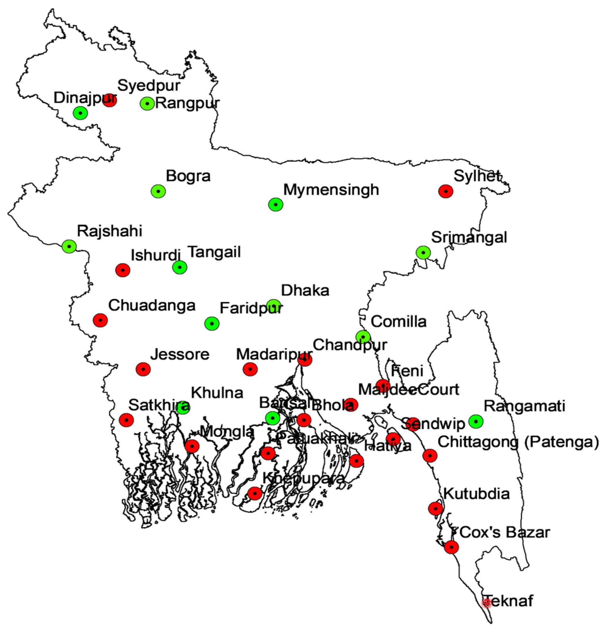
3. Study Region and Data

Bangladesh is a tropical country, situated mainly in the deltas of large rivers flowing from the Himalayas. The Brahmaputra River, known locally as the Jamuna, unites with part of the Ganges to form the Padma, which, after it merges with the third largest river, the Meghna, flows into the Bay of Bengal. No part of the delta area is more than 150 m above the sea level, with most of it being just a meter or two above sea level. During the rainy season, flood water covers most of the land surface, damaging crops and injuring the economy. The northwestern section of the country, drained by the Teesta River, is somewhat higher and less flat, but the only really hilly regions are in the east, notably in the Chittagong Hill Tracts to the southeast and the Sylhet district to the northeast. We collected observed data for soil temperature at different depths, air temperature, sunshine duration, rainfall, and humidity during 2001–2022 from 11 soil temperature observation stations in the Bangladesh Meteorological Department (Figure 1). Unfortunately, the observation of soil temperature is very limited in Bangladesh, which only takes place twice a day, so we could not simulate the diurnal temperature change in our study.

4. Forecast Experiment Design

In this study, we conducted a performance evaluation of five tree-based models (DT, RF, GBT, hybrid DT-GBT, and hybrid RF-GBT) in forecasting soil temperature at three depths (10 cm, 30 cm, and 50 cm) in Bangladesh. Our aim was to determine the optimal tree-based forecast model for soil temperatures in Bangladesh by inputting different meteorological factors. Since different lead times, time window sizes, and input scenarios play key roles in the accuracy of soil temperature forecasting in Bangladesh, we considered the following cases:
Three types of lead times: one day, three days, and five days.
Five sizes of time window: one day, two days, three days, four days, and five days.
Eight combinations of daily minimum temperature (MIN), i.e., daily maximum temperature (MAX), daily mean temperature (MEAN), daily sunshine duration (SUN), daily rainfall (RAIN), and daily humidity (HUM), were used as model inputs. In particular, the combinations were as follows: (1) MEAN, (2) MEAN-SUN, (3) MEAN-MAX-MIN, (4) MEAN-HUM-RAIN, (5) MEAN-MAX-MIN-SUN, (6) MEAN-MAX-MIN-SUN-RAIN, (7) MEAN-MAX-MIN-SUN-HUM, and (8) MEAN-MAX-MIN-SUN-HUM-RAIN.
In almost all machine learning studies, the partition of training and testing datasets follows a 70–30 split rule ([11]), so the soil temperature dataset in Bangladesh was divided as follows: the data covering the period from 1 January 2001 to 31 December 2015 were used for the training dataset, and the data covering the period from 1 January 2016 to 31 December 2022 were used for the testing dataset.

5. Results and Discussion

Bangladesh has 11 soil temperature observation stations. From 2001 to 2022, at a depth of 10 cm (ST10), the soil temperature ranged from 13.4 °C to 35.2 °C. At a 30 cm depth (ST30), it ranged from 15 °C to 34.7 °C, and at a 50 cm depth (ST50), it ranged from 15.1 °C to 34.6 °C. Affected by large oscillations in air temperature, the variability of ST10 was significantly larger than that of ST30 and ST50.
Figure 2 further illustrates the average daily soil temperature variations at three distinct depths across the 11 soil monitoring stations in Bangladesh. The average daily soil temperature at the 10 cm depth varies from 17.1 °C (Dhaka station) to 32.9 °C (Rajshahi station); at the 30 cm depth, it varies from 18.07 °C (Dinajpur station) to 32.7 °C (Dhaka station); and at the 50 cm depth, it varies from 18.6 °C (Dinajpur station) to 32.4 °C (Faridpur station). The overall range of average temperatures across the stations is from 18.2 °C to 31.3 °C for ST10, from 19.09 °C to 30.9 °C for ST30, and from 19.7 °C to 30.6 °C for ST50. Soil temperatures at Rangamati, Srimongal, Dhaka, and Barisal exhibit nearly identical temperatures across all depths, whereas soil temperatures at various depths at stations like Tangail and Bogra have significant differences. At most of the stations, the soil at the 10 cm depth has higher temperatures in January–August and lower temperatures in September–December compared to those at the 30 cm and 50 cm depths. The main reason for this is that surface soil temperature is more susceptible to temperature fluctuations. Specifically, the soil layer at the 10 cm depth exhibits greater sensitivity to short-term fluctuations and seasonal variations due to its proximity to the surface and limited thermal mass, whereas deeper soil layers at 30 cm and 50 cm exhibit more stable temperature trends due to their insulation from surface-level conditions. Aligning with the changing seasons, soil temperature at all depths shows increasing trends from January to April, and decreasing trends from September to December. The soil temperature from May to August is the highest in the whole year, which is consistent with the summer season. These temperature variations are primarily attributed to seasonal shifts in the solar insolation, daylight duration, and thermal inertia of the soil.

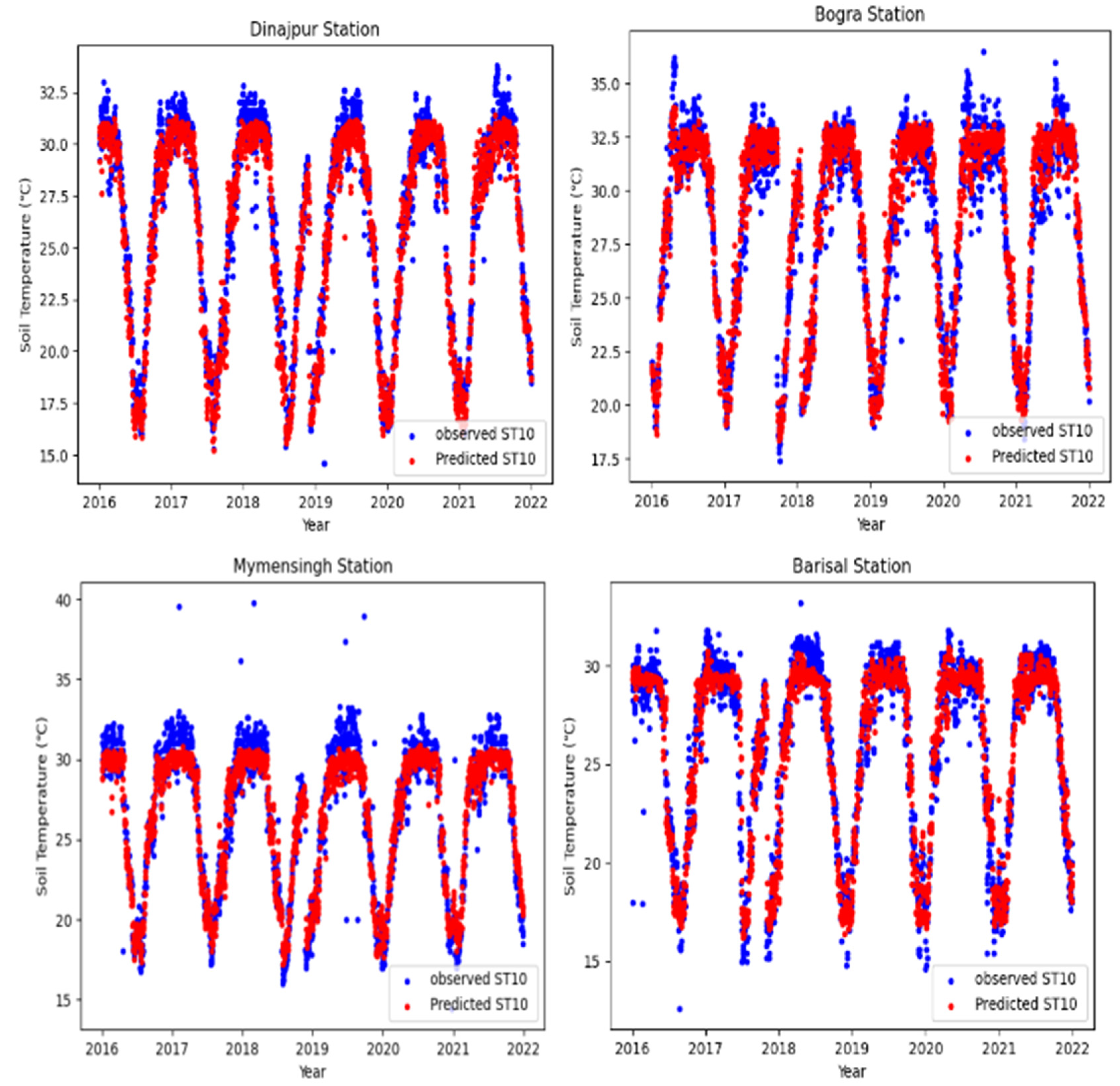
5.1. Forecasting Soil Temperature at 10 cm Depth in Bangladesh

We combined three types of lead times, five sizes of time windows, eight input scenarios, and five tree-based models to forecast soil temperature at the depth of 10 cm (ST10), and then revealed the optimal combination of the tree model, time window, and input scenario in forecasting ST10. The model performance was evaluated using the root mean squared error (RMSE) and Pearson correlation coefficient (R).

5.1.1. One-Day Lead-Time Forecast

In the context of one-day lead-time forecasting of soil temperature at 10 cm depth, Table 1 and Table 2 evaluate tree-based model performance across various scenarios, emphasizing accuracy based on low errors and strong correlations between forecast and actual values. This provided some insights into understanding the complex relationships between meteorological factors and soil temperature fluctuations.
Forecast by DT: In terms of average RMSE and R values, from Table 1 and Table 2, it is clear that the forecast accuracy of the testing datasets is a little worse than that of the training datasets. For the testing dataset, the DT model with the third input scenario achieved the best forecast, consistently showing the lowest average RMSE values (ranging from 2.086 °C to 2.126 °C) and the highest average R values (ranging from 0.932 to 0.936) across various time window sizes. The smallest time window and the simplest input scenario exhibited the lowest average R and highest average RMSE values. As the size of the time window increased, the forecast accuracy of the model increased. This means that the DT model is sensitive to the input parameters and time window sizes.
Forecast by RF: The forecast performance of the RF model with different input scenarios and different sizes of time window for the training dataset and testing datasets is demonstrated in Table 1 and Table 2, respectively. It is clear that the forecast accuracy of the testing datasets is a little worse than that of the training datasets. For the testing dataset, the eighth input scenario, which combined all meteorological factors, yielded the best forecast accuracy when the size of the time window was one day, two days, three days, or five days, whereas the seventh input scenario performed best when the size of the time window was four days. Compared with DT, the RF achieved a slight improvement in the RMSE and R values. The lowest average RMSE value (1.994 °C) was achieved with the combination of the eighth input scenario and the largest time window.
Forecast by GBT: The forecasting accuracy of the GBT model was consistent between the testing and training datasets, with the same optimal time window and input scenarios. For the testing dataset, the forecast by GBT showed a consistent trend where the average RMSE values increased with larger time windows, although the forecast performance varied with different input scenarios. The best GBT model utilizing all meteorological parameters (eighth scenario) and the largest time window achieved the lowest average RMSE (1.976 °C) and the highest average R value (0.945). When the size of the time window was reduced from five days to one day, the average RMSE value increased from 1.976 °C to 2.067 °C, and the average R value decreased from 0.945 to 0.937.
Forecast by Hybrid DT-GBT: The forecast accuracy of the training data was slightly higher than that of the testing dataset. For the testing dataset, the combination of all meteorological factors as the model input consistently led to the lowest average RMSE value and the highest average R value. The hybrid structure excels in capturing complex relationships, especially achieving the lowest average RMSE of 1.994 °C when the size of the time window was set to three days, and the highest average R value (0.944) when the size of the time window was set to five days.
Forecast by Hybrid RF-GBT: The results of the hybrid RF-GBT’s forecast performance in terms of the average RMSE and R values from all soil temperature observation stations are shown in Table 1 and Table 2. For the hybrid model, the prediction results were consistent for the testing and training datasets. The differences in terms of R and RMSE values indicated that the model’s performance was more robust in training processing. For the testing dataset, the eighth input scenario led to the best forecast under all time window sizes, achieving the best prediction with the lowest average RMSE (1.973 °C) and the highest average R (0.945) when the time window size was set to five.
Best combination for one-day lead-time forecast: The combination of hybrid RF-GBT, eighth input scenario, and five-day time window achieved the best forecast performance with the lowest average RMSE (1.973 °C) and the highest average R (0.945). Figure 3 demonstrates strong agreement between the optimal predictions and actual observations at the four soil temperature observation stations. When the time window was reduced to four days, the best forecast was achieved by the combination of GBT and the eighth input scenario. Similarly, at three-day, two-day, and one-day time windows, the best predictions were obtained using GBT, hybrid RF-GBT, and GBT, respectively. This underscored the best forecasting capability of the hybrid RF-GBT and GBT for soil temperature at a 10 cm depth. Generally, the best combination of model, input scenario, and time window can properly capture the oscillation patterns of soil temperature at the 10 cm depth in the frame of a one-day lead-time forecast, but it cannot capture some extreme high/low soil temperatures. At the same time, some outliers in the observed soil temperature data (e.g., unusually high and low soil temperatures at the Barisal station) are likely caused by measurement errors.

5.1.2. Three-Day Lead-Time Forecast

Table 3 shows the evaluation of the five tree-based models’ performance under various input scenarios and time windows on the testing datasets. For DT forecasts, the MEAN-MAX-MIN input scenario under a five-day time window achieved good accuracy. When the size of the time window decreased from five days to one day, the forecast accuracy increased an average RMSE from 1.849 °C to 1.885 °C and decreased the average R value from 0.918 to 0.915. For RF forecasts, the sixth input scenario performed better than other input scenarios, except for the one-day time window; in particular, it achieved the lowest average RMSE (1.759 °C) and the highest average R (0.926) under the five-day time window. The GBT forecasts showed improved performance when larger time windows were applied. The eighth input scenario consistently achieved the highest accuracy under all time windows, with the lowest average RMSE (1.755 °C) and the highest average R (0.926) demonstrating strong predictive capability. For the hybrid DT-GBT forecast, the sixth input scenario yielded the lowest average RMSE and the highest average R values under one/two/three-day time windows, whereas the eighth input scenario yielded the best forecast under a four-day time window. Under a five-day time window, the eighth input scenario yielded the lowest average RMSE and the highest average R value. The hybrid RF-GBT achieved the lowest average RMSE of 1.752 °C and the highest average R value of 0.927 under a five-day time window using all input factors.
Best combination for three-day lead-time forecast: The hybrid RF-GBT model utilizing all input factors under a five-day time window excelled among all combinations of model, input, and time widows. It achieved the lowest average RMSE (1.752 °C) and the highest average R value (0.927). In Figure 4, the soil temperature forecast by the hybrid RF-GBT model closely matched the observed data at the Dinajpur, Barisal, Mymensingh, and Bogra stations, especially most of the lowest soil temperature data were well captured using the hybrid RF-GBT. The observed extremely high soil temperature at the Mymensingh station was clearly bought by abnormal measuring instruments.

5.1.3. Five-Day Lead-Time Forecast

Similar to Section 5.1.1 and Section 5.1.2, we compare the forecast performance of five tree-based models under different input scenarios and time windows on the testing dataset. In order to avoid the repetition of similar tables, we only report the main results here. The DT model exhibited good performance in forecasting soil temperature, and the combination of the MEAN-MAX-MIN input scenario, and four-day time window demonstrated the lowest average RMSE of 1.995 °C and the highest average R value of 0.902. Although a one-day time window always exhibited lower accuracy with mean input parameters, the largest time window did not produce the best accuracy. For RF forecasts, the sixth input scenario performed the best under all time windows; in particular, the lowest average RMSE (1.910 °C) and highest average R (0.911) were reached under a four-day time window. The GBT model with the eighth input scenario achieved the highest accuracy under various time windows. Among them, the use of a four-day time window yielded the lowest average RMSE (1.915 °C) and the highest average R (0.910). In the forecast performance of the hybrid DT-GBT, the use of the sixth input scenario and a four-day time window achieved the lowest average RMSE (1.936 °C) and the highest average R (0.908) values. The best hybrid RF-GBT forecast consistently adopted the eighth input scenario for all time windows. The combination of the eighth input scenario and four-day time window achieved the lowest average RMSE value (1.908 °C) and the highest average R value (0.911).
Best combination for five-day lead-time forecast: The hybrid RF-GBT, utilizing all the input factors under a four-day time window, emerged as the optimal performing model with the largest average R value (0.911) and the lowest average RMSE value (1.908 °C). Figure 5 demonstrates that the forecast of the hybrid RF-GBT under a four-day time window offered a close fit with the observed values and superior accuracy at the Dinajpur, Borga, Mymensigh, and Bariasal stations. The hybrid RF-GBT model properly captured the oscillation patterns of soil temperature, but it provided a clear underestimate of extremely high soil temperatures. At the same time, some unusually high observed soil temperatures in Mymensingh were caused by measurement errors.

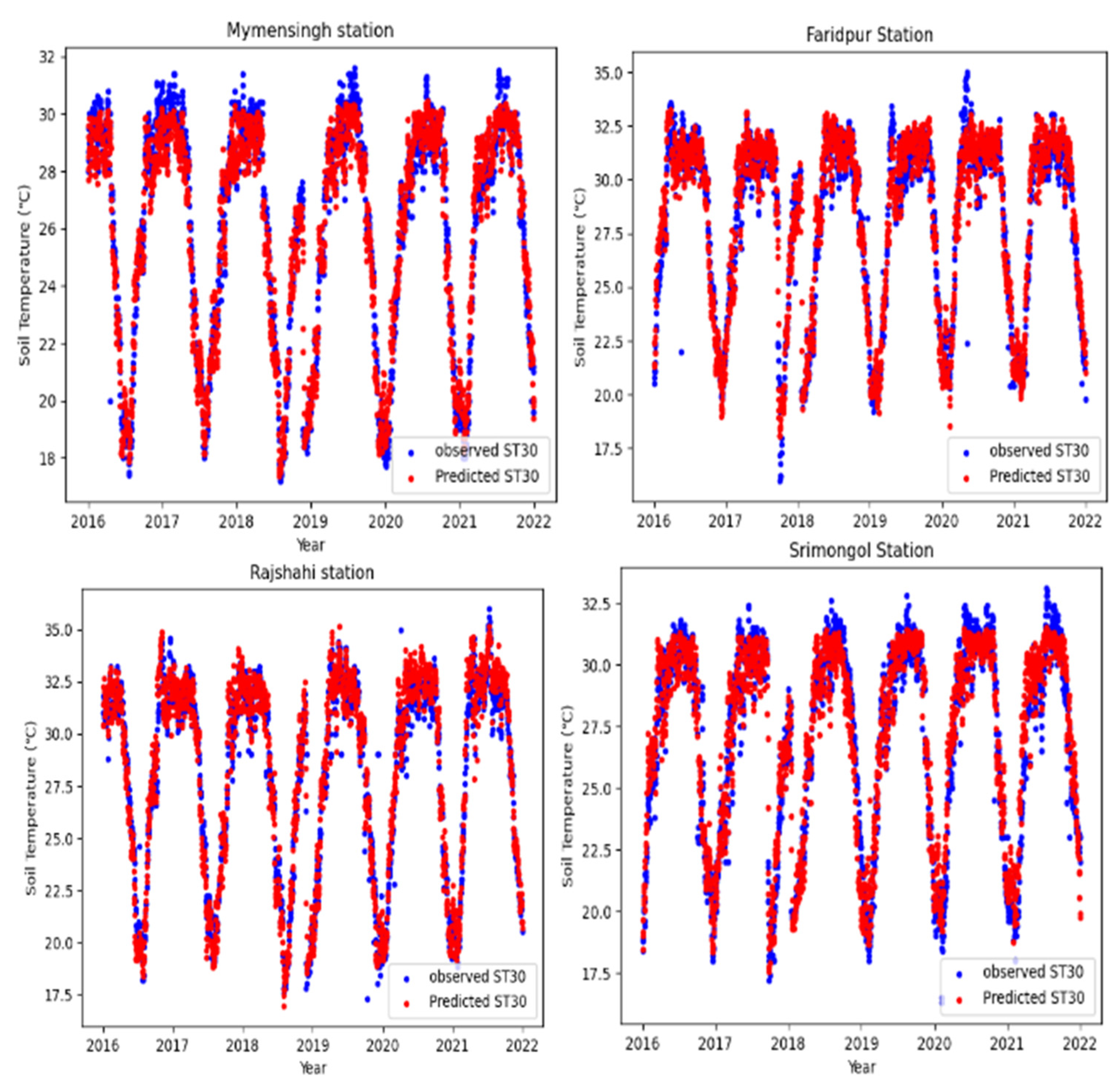
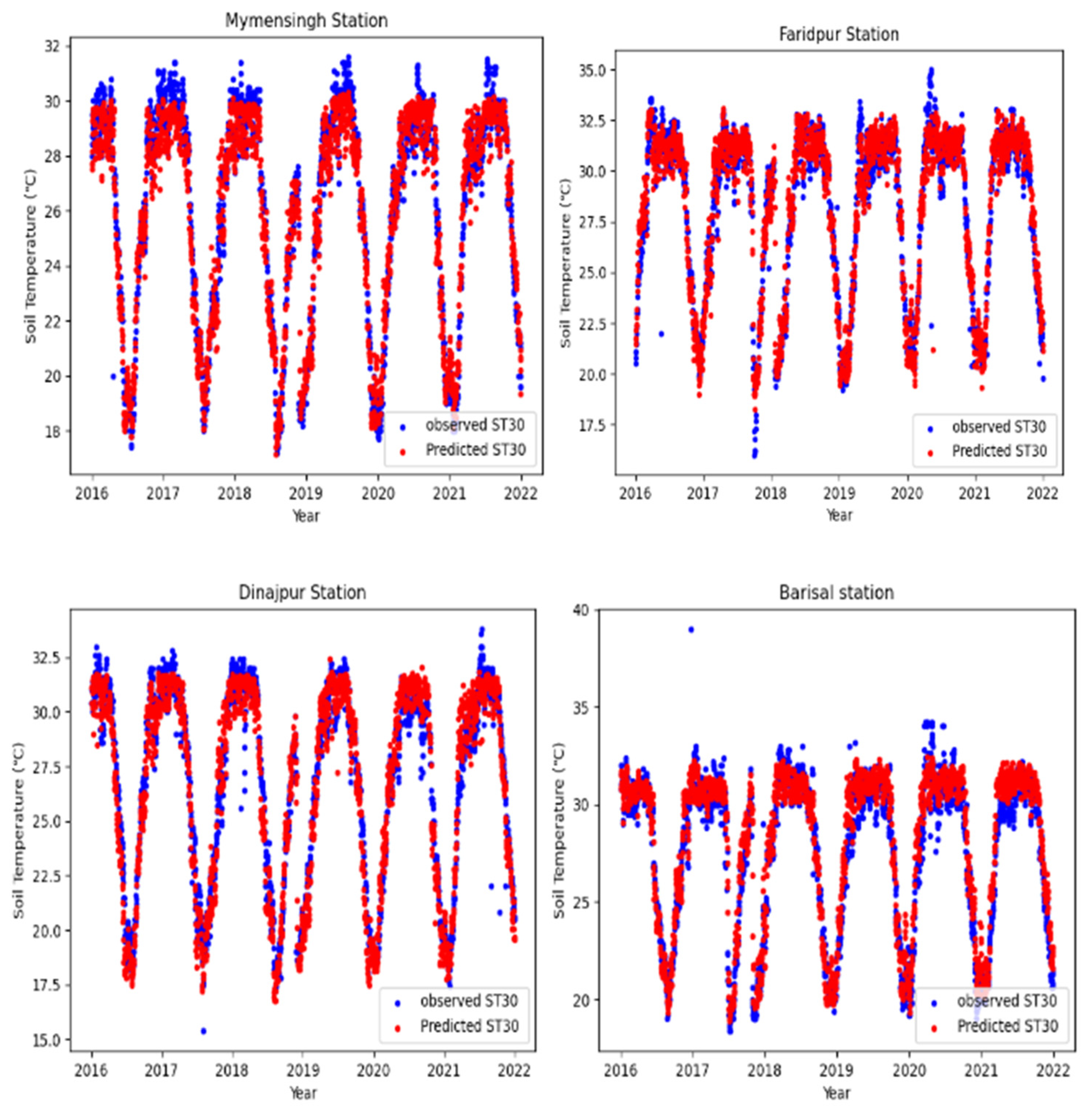
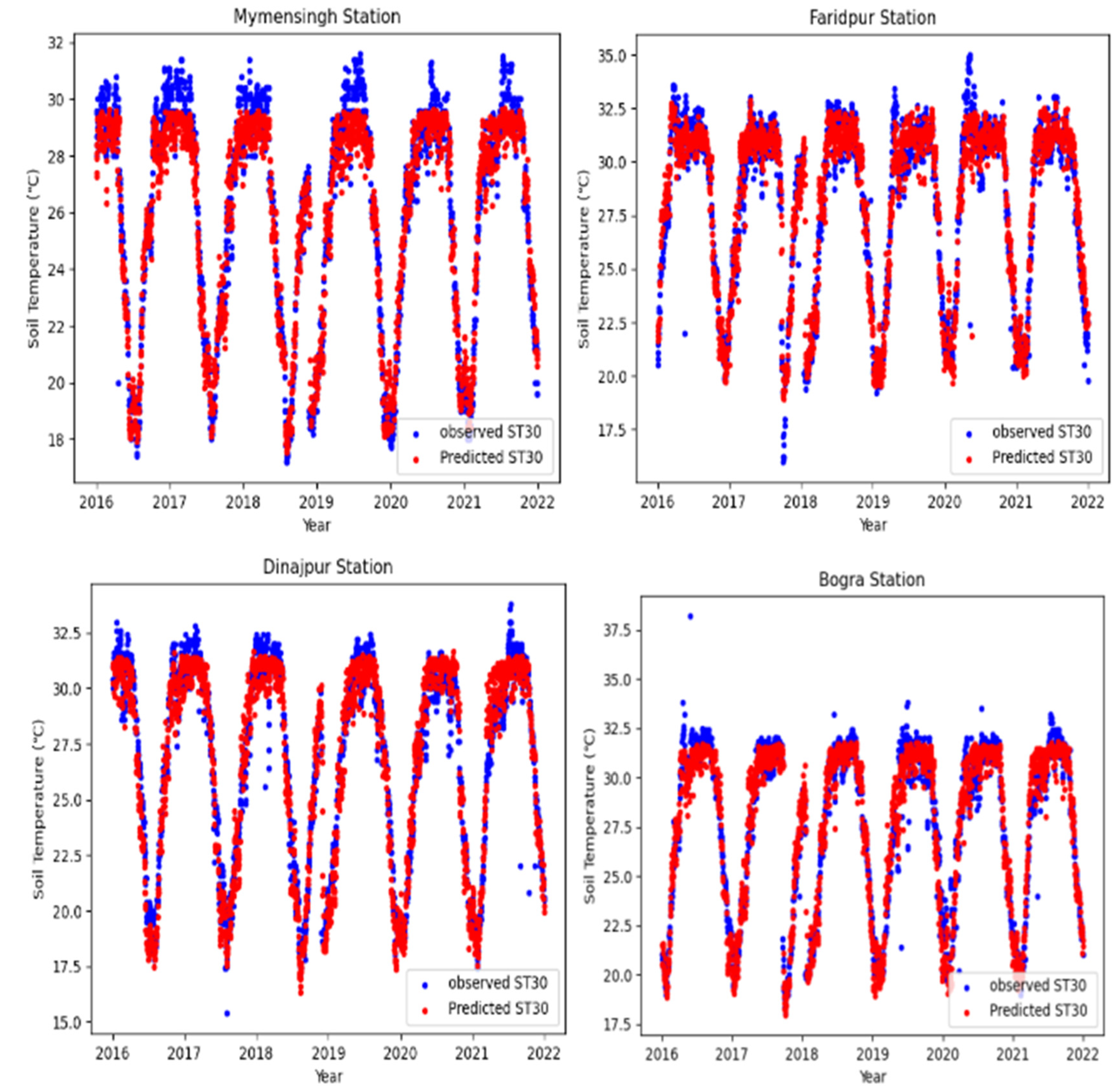
5.2. Forecasting Soil Temperature at 30 cm Depth in Bangladesh

Similar to Section 5.1, we combined the three types of lead times, five sizes of time windows, eight input scenarios, and five tree-based models to predict soil temperatures at the depth of 30 cm (ST30) in order to show the optimal combination of a tree model, time window, and input scenario in forecasting soil temperature. The model performance was also evaluated using root mean squared error (RMSE) and Pearson correlation coefficient (R).

5.2.1. One-Day Lead-Time Forecast

Table 4 demonstrates five tree-based models’ performance under various time windows and input scenarios on the testing dataset. The DT model achieved the best forecast with the MAX-MIN-MEAN input scenario under a five-day time window, showing the lowest average RMSE value (1.349 °C) and the highest average R value (0.950). Compared with DT, the RF achieved a slight improvement in terms of RMSE and R values; in particular, the use of a five-day time window achieved the lowest average RMSE (1.225 °C) and the highest average R (0.959). The forecast performance of GBT utilizing all meteorological parameters and the largest time window achieved the lowest average RMSE (1.193 °C) and the highest average R value (0.961). The hybrid models, DT-GBT and RF-GBT, consistently performed well using the combination of all meteorological factors as inputs, thereby achieving the lowest average RMSE and the highest average R values and demonstrating their effectiveness and complex relationship-capturing capabilities. The hybrid DT-GBT model achieved the lowest average RMSE (1.223 °C) and the highest average R value (0.959) when the size of the time window was set to four days. The hybrid RF-GBT, using the eighth input scenario and a five-day time window consistently resulted in the lowest average RMSE (1.188 °C) and the highest average R value (0.962).
Best combination for one-day lead-time forecast: The combination of hybrid RF-GBT, eighth input scenario, and five-day time window achieved the best forecast performance with the lowest average RMSE (1.188 °C) and the highest average R (0.962). The second-best forecast combination adopted the four-day time window, followed by three-day, two-day, and one-day time windows, using the eighth input scenario and the hybrid RF-GBT. This highlights the superior forecast capability of the hybrid RF-GBT for soil temperature at 30 cm depth. Figure 6 demonstrates a strong agreement between optimal predictions and actual observations of ST30 at four observation stations. Compared with forecasting ST10, extremely high temperature was captured better in ST30.

5.2.2. Three-Day Lead-Time Forecast

In parallel with the one-day lead-time forecast at a 30 cm depth, we assess the forecast performance of five tree-based models within a three-day lead-time framework. In order to avoid the repetition of similar tables, we only report the main accuracy results on the testing datasets. The DT model achieved the lowest average RMSE of 1.389 °C and the highest average R value of 0.946 under the combination of the third input scenario and a five-day time window. In the case of RF forecasts, the eighth scenario consistently performed better than other input scenarios across all time windows. The corresponding average RMSE ranged from 1.287 °C to 1.40 °C, the average R value ranged from 0.944 to 0.954, and the use of a five-day time window produced the best forecast results. The GBT showed improved performance with larger time windows, achieving the lowest average RMSE (1.261 °C) and the highest average R value (0.955) when using the eighth input scenario and a five-day time window. The hybrid DT-GBT model also performed well with the eighth input scenario and a five-day time window. The hybrid RF-GBTs exhibited the strongest performance, particularly achieving the lowest average RMSE of 1.260 °C and the highest average R value of 0.956 under a five-day time window and using all meteorological factors.
Best combination for three-day lead-time forecast: The hybrid models, especially RF-GBT, stood out for their strong performance, particularly with larger time windows and eighth input scenarios. It achieved the lowest average RMSE (1.260 °C) and the highest average R value (0.956). Figure 7 demonstrates a strong agreement between optimal predictions by RF-GBT and actual observations at four soil temperature observation stations. Such a visual comparison confirmed that the RF-GBT hybrid model is highly capable of providing accurate and reliable predictions.

5.2.3. Five-Day Lead-Time Forecast

Similar to Section 5.2.2, in order to avoid the repetition of similar tables, we only report the main accuracy results on the testing datasets. For DT forecasts, the MEAN-MAX-MIN input scenario under a four-day time window produced the highest accuracy with the lowest average RMSE of 1.496 °C and the highest average R value of 0.935. Interestingly, a one-day time window consistently exhibited lower accuracy with the mean input parameters, but the largest time window size did not produce the best prediction. For RF forecasts, the sixth scenario performed the best across all time windows except for the one-day time window, with the lowest average RMSE (1.407 °C) and the highest average R (0.943) under a five-day time window. The performance of GBT varied across different input scenarios and time windows, with the eighth input scenario demonstrating the highest accuracy, particularly with a four-day time window, resulting in the lowest average RMSE (1.399 °C) and the highest average R value (0.944). For the hybrid DT-GBT forecasts, the use of the sixth and eighth input scenarios produced the smallest RMSE and largest R values for each time window, with the most favorable results observed with a four-day time window, achieving the lowest average RMSE (1.427 °C) and the highest average R (0.941) value. The hybrid RF-GBT forecasts consistently favored the eighth input scenario for all time windows, except the four-day time window. The combination of the eighth input scenario and a five-day time window resulted in the lowest average RMSE (1.398 °C) and the highest average R (0.945) value.
Best combination for five-day lead-time forecast: The hybrid RF-GBT utilizing all input parameters under the five-day window emerged as the optimal forecast model in terms of the lowest average RMSE value (1.398 °C), and the largest average R value (0.945). This signifies the model’s strong ability to capture and predict soil temperature variations accurately. Figure 8 demonstrates that the hybrid RF-GBT under a five-day time window offered a close match with the observed values and exhibited superior accuracy. A closer analysis of the figures reveals that errors mainly occurred in the forecast of extremely high soil temperature.

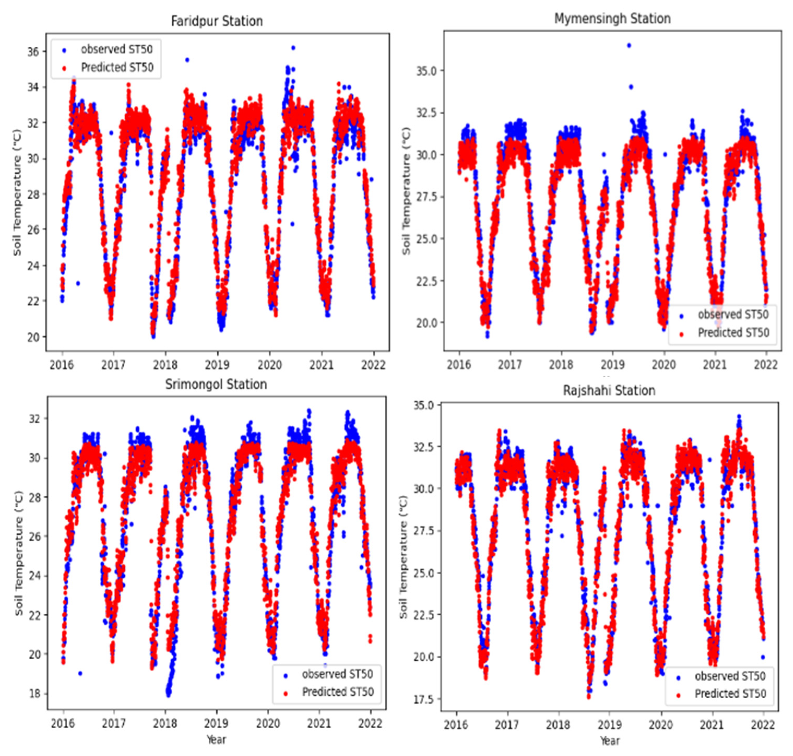
5.3. Forecasting Soil Temperature at 50 cm Depth in Bangladesh

In this subsection, based on the model performance of the testing dataset, we explored the optimal combination of tree-based models, time windows, and input scenarios in forecasting soil temperature at the depth of 50 cm (ST50).

5.3.1. One-Day Lead-Time Forecast

In the context of one-day lead-time soil temperature forecasting at 50 cm depth, Table 5 presents an evaluation of the performance of the tree-based model, emphasizing accuracy through low errors and strong correlations between the predicted and actual values. The DT model achieved the best forecast with the third and seventh input scenarios, consistently showing the lowest average RMSE values (2.001 °C to 2.139 °C) and the highest average R values (0.912 to 0.926) across various sizes of time windows. For the RF forecasts, the eighth input scenario was optimal for one-day, two-day, and three-day time windows, whereas the third and eighth input scenarios performed best for the five-day time window. It achieved slight improvement in terms of average RMSE (1.893 °C to 2.079 °C) and average R values (0.920 to 0.941) for each time window. In the case of the GBT, the third and eighth input scenarios achieved the lowest average RMSE (1.897 °C) and the highest average R value (0.941). When the size of the time window was reduced from five days to one day, the average RMSE value increased from 1.897 °C to 2.091 °C, and a decrease in the average R value declined from 0.941 to 0.919. The hybrid DT-GBT consistently achieved the lowest average RMSE with the third input scenario and the highest average R value with the eighth input scenario. Notably, under the five-day time window, the DT-GBT model demonstrated good RMSE (1.920 °C) and R (0.937). Similarly, the hybrid RF-GBT consistently favored the eighth input scenario for all time-window sizes, achieving the lowest average RMSE (1.888 °C) and the highest average R value (0.942) with a five-day time window.
Best combinations for one-day lead-time forecast: In a one-day lead-time forecasting of ST50, the combination of hybrid RF-GBT, eighth input scenario, and five-day time window achieved the best forecast performance with the lowest average RMSE (1.888 °C) and the highest average R (0.942). For four-day, three-day, and two-day time windows, the best predictions were obtained with the hybrid RF-GBT, and a one-day time window with the RF, respectively. This underscored the superior forecast capability of the hybrid RF-GBT and RF for soil temperature at 50 cm depth. Figure 9 illustrates successful one-day advanced soil temperature forecasting for four stations, showing strong alignment between model predictions and observed values. The optimal model properly captured main soil temperature changes; moreover, it accurately forecasted extremely high soil temperatures at the Faridpur and Rajshahi stations.

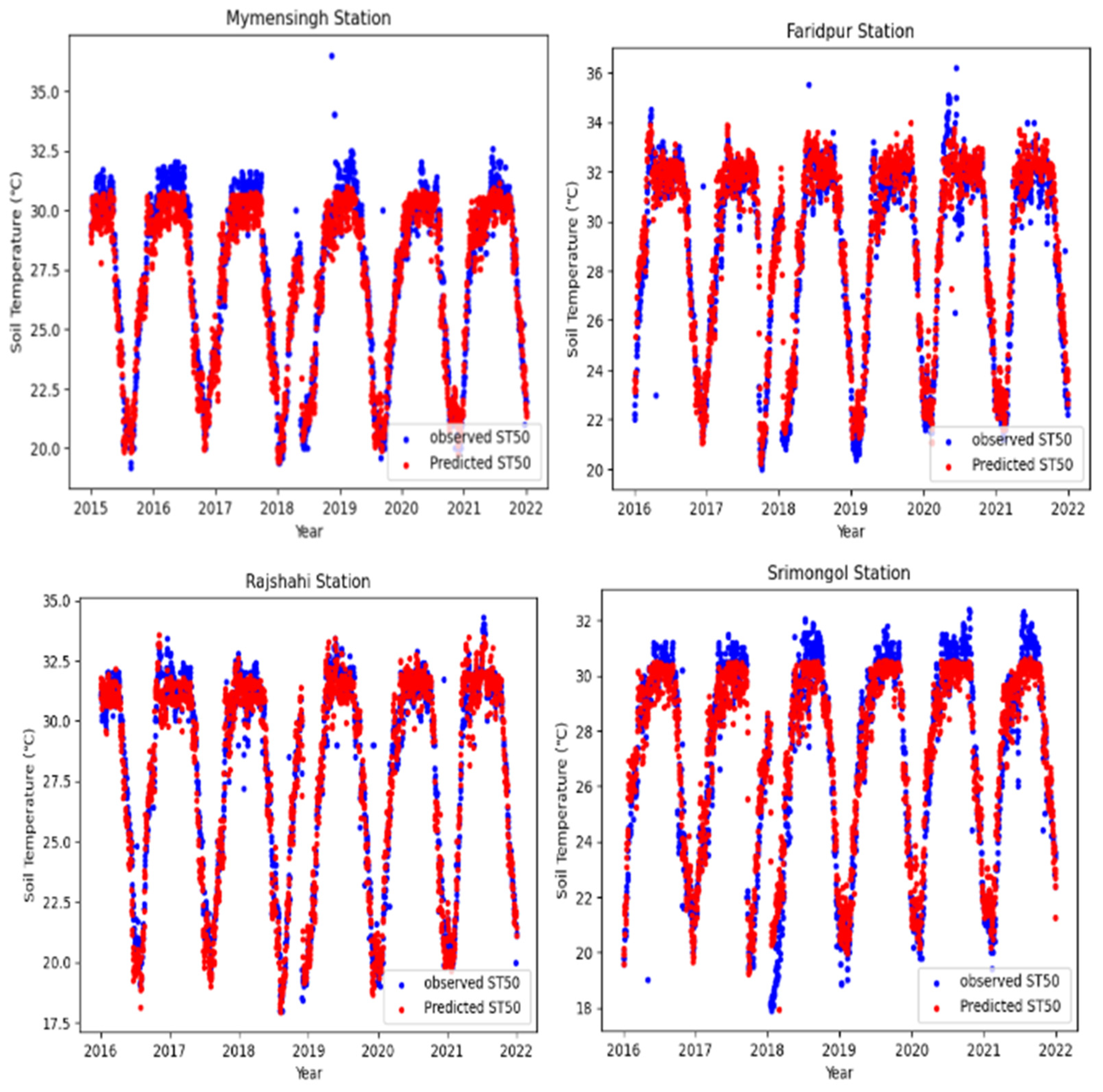
5.3.2. Three-Day Lead-Time Forecast

Similar to Section 5.3.1, in order to avoid the repetition of similar tables, we only report the main accuracy results on the testing datasets. The DT model produced good accuracy when the third input scenario and a five-day time window size were adopted. The RF forecasts using the third and eighth input scenarios consistently performed better than the other input scenarios. It achieved an average RMSE ranging from 1.906 °C to 2.04 °C and an average R value ranging from 0.925 to 0.940, where the five-day time window showed the best forecast results. The GBT with the third or eighth input scenario consistently achieved the highest accuracy under all time windows, with the lowest average RMSE (1.903 °C) and the highest average R (0.939). The performance of the hybrid DT-GBT consistently delivered the lowest average RMSE with the third input scenario and achieved the highest average R values with the eighth input scenario across all time windows. In particular, under a five-day time window, the third input scenario yielded the lowest average RMSE, and the eighth input scenario yielded the highest average R value. Similarly, the hybrid RF-GBT with the third and eighth input scenario led to the best forecast under all time-window sizes, achieving the best prediction with the lowest average RMSE (1.901 °C) and the highest average R value (0.940) when using a five-day time-window.
Best combination for three-day lead-time forecast: The combination of hybrid RF-GBT, third and eighth input scenario, and five-day time window achieved the best forecast performance of ST50 with the lowest average RMSE (1.901 °C) and the highest average R (0.940), respectively. This underscored the best forecast capability of the hybrid RF-GBT for soil temperature at 50 cm depth. These models, employing the third and eighth input parameter combination in the five-day time window, provided the best predictions. Figure 10 demonstrates a strong agreement between optimal predictions and actual observations at four soil temperature observation stations. In particular, the forecast at the Mymensingh station exhibited a minor underestimation, whereas the forecast at the Srimongal station demonstrated a combination of slight overestimation and underestimation.

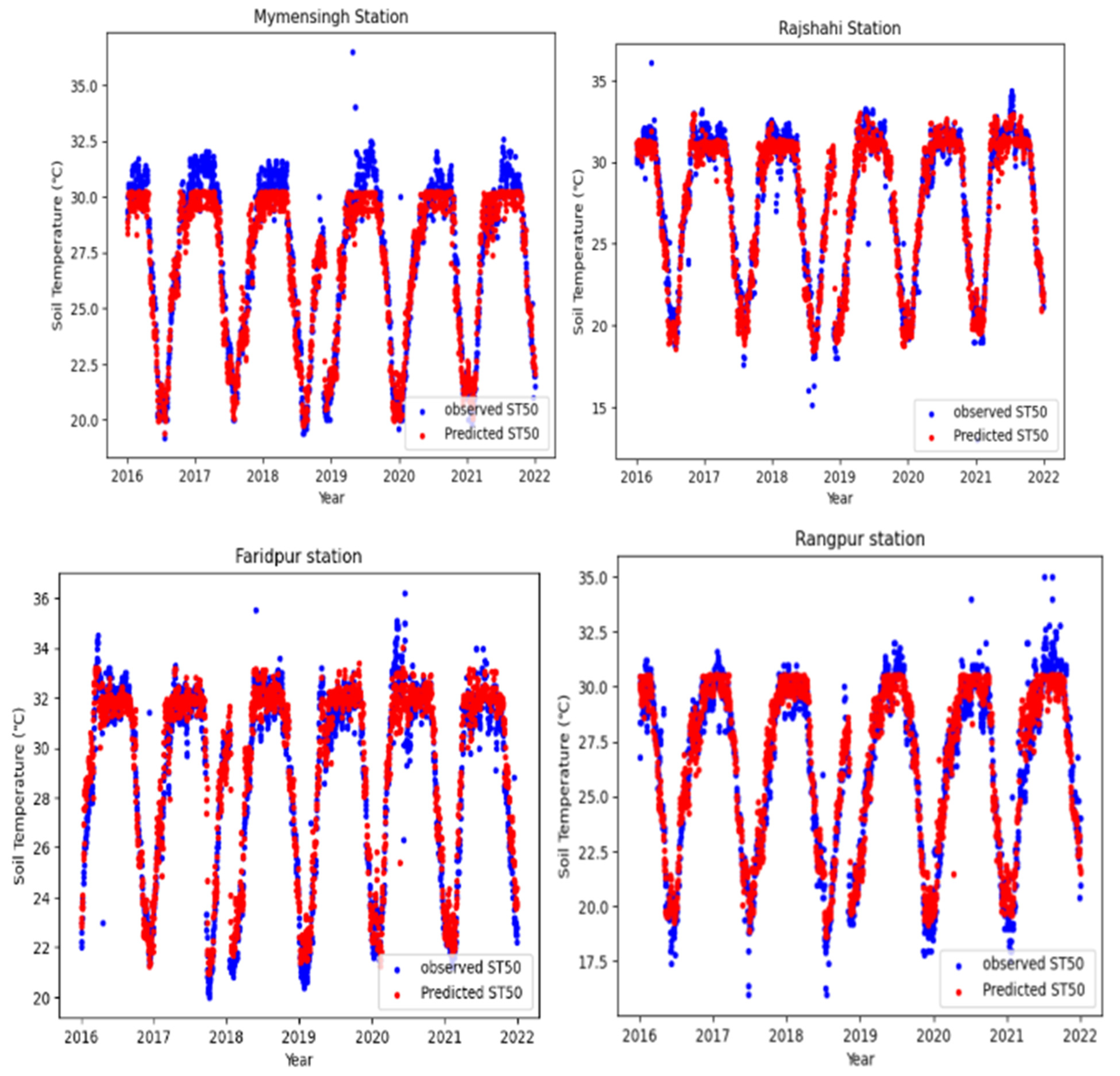
5.3.3. Five-Day Lead-Time Forecast

Similar to Section 5.3.1, in order to avoid the repetition of similar tables, we only report the main accuracy results on the testing datasets. The DT model achieved the lowest average RMSE (2.046 °C) and the highest average R value (0.921) under MEAN-MAX-MIN input scenario and a five-day time window. The RF model demonstrated the best performance under the third and eighth input scenarios, resulting in the lowest average RMSE (1.962 °C) and the highest average R (0.935). The GBT model using the third and eighth input scenarios achieved the highest accuracy under various time windows; in particular, a five-day time window achieved the lowest average RMSE (1.971 °C) and the highest average R value (0.931). In the case of the hybrid DT-GBT, the third and eighth input scenarios produced the smallest average RMSE and the largest average R values for each time window. Similarly, the hybrid RF-GBT consistently relied on the third and eighth input scenarios for all time windows. For RF-GBT forecast under a five-day time window, the third input scenario yielded the lowest average RMSE value (1.970 °C) and the eighth input scenario yielded the highest average R value (0.933).
Best combination for five-day lead-time forecast: The above comparison highlighted that the RF, utilizing third and eighth input factors under a five-day time window, emerged as the optimal forecasting model with the lowest average RMSE value (1.962 °C) and the largest average R value (0.935). Figure 11 demonstrates that the RF under a five-day time window offered a close fit with the observed values and superior accuracy at four stations. The main oscillation patterns of soil temperature were well captured, except for some of the highest/lowest soil temperature values.

6. Conclusions

Bangladesh faces significant challenges in adapting to the impact of climate change and is often cited as one of the most vulnerable countries to climate change ([32,33]). Since soil temperature complexities have far-reaching effects on agriculture, influencing anything from root development to microbial activity, change patterns of soil temperature are of great importance for an agro-based economy like Bangladesh. Soil properties, such as texture, moisture content, and organic matter, work together to determine the flow of heat through the Earth, influencing temperature changes. The process-oriented, physics-based models incorporate these soil properties into the forecasting process. Compared with this modeling approach, machine learning can only provide limited insight into understanding soil dynamic changes. However, due to the lack of enough observation datasets to drive process-oriented, physics-based models in poor countries like Bangladesh, machine learning has become a more effective and low-cost quantitative approach.
Choosing the optimal model for soil temperature forecasting is not one-size-fits-all. More input variables and more complex models cannot guarantee a high forecast performance. It must involve a careful evaluation of the specific requirements, resources, and constraints of the application to make an informed decision about which model is best suited for the task. In this study, we explored the combination of five tree-based models, eight input scenarios, and five sizes of time windows to forecast soil temperature at 10 cm/30 cm/50 cm depth under three types of lead times. The five tree-based models, including DT, GBT, RF, hybrid DTGBT, and hybrid RF-GBT, were evaluated for one-day, three-day, and five-day lead-time forecasts in terms of both RMSE and R values. The optimal combination to produce the best soil temperature forecast and related accuracy are shown in Table 6. The hybrid RF-GBT model with the eighth input scenario and five-day time window is optimal for forecasting soil temperature at the depth of 10 cm and 30 cm, whereas the RF model with the eighth input scenario and five-day time window is optimal for forecasting soil temperature at the depth of 50 cm when the lead time is long (five days). The best accuracy of soil temperature at depths of 10 cm, 30 cm, and 50 cm were RMSE:1.752 °C and R:0.945; RMSE: 1.188 °C and R: 0.962; RMSE: 1.888 °C and R: 0.942, respectively.
Since our study includes the first soil temperature forecast model from meteorological observations in Bangladesh, it will save the soil observation cost significantly, fill in missing soil temperature observations, and enhance the accessibility and accuracy of soil temperature data, making it especially valuable for research and informed decision-making in Bangladesh. At the same time, it provides valuable insights for agricultural soil management, fertilizer application, and water resource optimization in Bangladesh, as well as in other South Asian countries that share the same climate patterns as Bangladesh.

Author Contributions

L.C.D. and Z.Z. are co-first authors. Conceptualization, Z.Z.; methodology, Z.Z. and L.C.D.; software, L.C.D.; validation, L.C.D.; formal analysis, Z.Z. and L.C.D.; investigation, L.C.D.; resources, L.C.D.; data curation, L.C.D.; visualization, L.C.D.; writing—original draft preparation, Z.Z. and L.C.D.; writing—review and editing, Z.Z. and M.J.C.C. All authors have read and agreed to the published version of the manuscript.

Funding

The corresponding author was supported by the European Commission Horizon 2020 Framework Program No. 861584 and the Taishan Distinguished Professor Fund No. 20190910.

Institutional Review Board Statement

Not applicable.

Informed Consent Statement

Not applicable.

Data Availability Statement

Data will be available upon a formal request to the corresponding author.

Conflicts of Interest

The authors declare no conflict of interest.

References

  1. Hu, G.; Zhao, L.; Wu, X.; Li, R.; Wu, T.; Xie, C.; Qiao, Y.; Shi, J.; Cheng, G. An analytical model for estimating soil temperature profiles on the Qinghai-Tibet plateau of China. J. Arid. Land. 2016, 8, 232–240. [Google Scholar] [CrossRef]
  2. Yan, Y.; Yan, R.; Chen, J.; Xin, X.; Eldridge, D.J.; Shao, C.; Wang, X.; Lv, S.; Jin, D.; Chen, J.; et al. Grazing modulates soil temperature and moisture in a Eurasian steppe. Agric. For. Meteorol. 2018, 262, 157–165. [Google Scholar] [CrossRef]
  3. Kandasamy, J.; Xue, Y.; Houser, P.; Maggioni, V. Performance of Different Crop Models in Simulating Soil Temperature. Sensors 2023, 23, 2891. [Google Scholar] [CrossRef] [PubMed]
  4. Seyfried, M.S.; Flerchinger, G.N.; Murdock, M.D.; Hanson, C.L.; Van Vactor, S. Long-term soil temperature database, Reynolds Creek experimental watershed, Idaho, United States. Water Resour. Res. 2001, 37, 2843–2846. [Google Scholar] [CrossRef]
  5. Qi, J.; Zhang, X.; Cosh, M.H. Modeling soil temperature in a temperate region: A comparison between empirical and physically based methods in SWAT. Ecol. Eng. 2019, 129, 134–143. [Google Scholar] [CrossRef]
  6. Gharabaghi, B.; Safadoust, A.; Mahboubi, A.; Mosaddeghi, M.; Unc, A.; Ahrens, B.; Sayyad, G. Temperature effect on the transport of bromide and E. coli NAR in saturated soils. J. Hydrol. 2015, 522, 418–427. [Google Scholar] [CrossRef]
  7. Tenge, A.; Kaihura, F.B.; Lal, R.; Singh, B. Diurnal soil temperature fluctuations for different erosion classes of an oxisol at Mlingano, Tanzania. Soil Tillage Res. 1998, 49, 211–217. [Google Scholar] [CrossRef]
  8. Sanikhani, H.; Deo, R.C.; Yaseen, Z.M.; Eray, O.; Kisi, O. Non-tuned data intelligent model for soil temperature estimation: A new approach. Geoderma 2018, 330, 52–64. [Google Scholar] [CrossRef]
  9. Holmes, T.R.H.; Owe, M.; De-Jeu, R.A.M.; Kooi, H. Estimating the soil temperature profile from a single depth observation: A simple empirical heat flow solution. Water Resour. Res. 2008, 44, W02412. [Google Scholar] [CrossRef]
  10. Albergel, C.; Dutra, E.; Muñoz-Sabater, J.; Haiden, T.; Balsamo, G.; Beljaars, A.; Isaksen, L.; de Rosnay, P.; Sandu, I.; Wedi, N. Soil temperature at ECMWF: An assessment using ground-based observations. J. Geophys. Res. Atmos. 2015, 120, 1361–1373. [Google Scholar] [CrossRef]
  11. Li, K.; Zhang, J.; Wu, L.; Yang, K.; Li, S. The role of soil temperature feed backs for summer air temperature variability under climate change over East Asia. Earth’s Future 2022, 10, e2021EF002377. [Google Scholar] [CrossRef]
  12. Song, Y.; Huang, A.; Chen, H. The Persistence and Reemergence of Atmospheric Anomaly Signals in Soil Temperature. J. Geophys. Res. Atmos. 2022, 127, e2022JD037218. [Google Scholar] [CrossRef]
  13. Di Salvo, C. Improving Results of Existing Groundwater Numerical Models Using Machine Learning Techniques: A Review. Water 2022, 14, 2307. [Google Scholar] [CrossRef]
  14. Chen, C.; Zhang, H.; Shi, W.; Zhang, W.; Xue, Y. A novel paradigm for integrating physics-based numerical and machine learning models: A case study of eco-hydrological model. Environ. Model. Softw. 2023, 163, 105669. [Google Scholar] [CrossRef]
  15. Bhagat, S.K.; Tung, T.M.; Yaseen, Z.M. Development of artificial intelligence for modeling waste water heavy metal removal: State of the art, application assessment and possible future research. J. Clean. Prod. 2020, 250, 119473. [Google Scholar] [CrossRef]
  16. Tung, T.M.; Yaseen, Z.M. A survey on river water quality modelling using artificial intelligence models: 2000–2020. J. Hydrol. 2020, 585, 124670. [Google Scholar]
  17. Zhang, Z.; Li, J. Big Data Mining for Climate Change; Elsevier: Amsterdam, The Netherlands, 2020. [Google Scholar]
  18. Schmidt, L.; Heße, F.; Attinger, S.; Kumar, R. Challenges in Applying Machine Learning Models for Hydrological Inference: A Case Study for Flooding Events Across Germany. Water Resour. Res. 2020, 56, e2019WR025924. [Google Scholar] [CrossRef]
  19. Okkan, U.; Ersoy, Z.B.; Kumanlioglu, A.A.; Fistikoglu, O. Embedding machine learning techniques into a conceptual model to improve monthly runoff simulation: A nested hybrid rainfall-runoff modeling. J. Hydrol. 2021, 598, 126433. [Google Scholar] [CrossRef]
  20. Alam, S.S.; Islam, A.J.; Hasan, M.M.; Rafid, M.N.M.; Chakma, N.; Imtiaz, M.N. Design and development of a low-cost IoT based environmental pollution monitoring system. In Proceedings of the 2018 4th International Conference on Electrical Engineering and Information & Communication Technology (iCEEiCT), Dhaka, Bangladesh, 13–15 September 2018; pp. 652–656. [Google Scholar]
  21. Uddin, M.S.; Istiaq, F.; Rasadin, M.; Talukder, R. Freshwater shrimp farm monitoring system for Bangladesh based on internet of things. Eng. Rep. 2020, 2, e12184. [Google Scholar] [CrossRef]
  22. Hasan, M.S.; Khandaker, S.; Iqbal, M.S.; Kabir, M.M. A real-time smart wastewater monitoring system using IoT: Perspective of Bangladesh. In Proceedings of the 2020 2nd International Conference on Sustainable Technologies for Industry 4.0 (STI), Dhaka, Bangladesh, 19–20 December 2020; pp. 1–6. [Google Scholar]
  23. Pathak, A.; AmazUddin, M.; Abedin, J.; Andersson, K.; Mustafa, R.; Hossain, M.S. IoT based Smart System to Support Agricultural Parameters: A Case Study. Procedia Comput. Sci. 2019, 155, 648–653. [Google Scholar] [CrossRef]
  24. Placidi, P.; Morbidelli, R.; Fortunati, D.; Papini, N.; Gobbi, F.; Scorzoni, A. Monitoring Soil and Ambient Parameters in the IoT Precision Agriculture Scenario: An Original Modeling Approach Dedicated to Low-Cost Soil Water Content Sensors. Sensors 2021, 21, 5110. [Google Scholar] [CrossRef] [PubMed]
  25. Morais, R.; Mendes, J.; Silva, R.; Silva, N.; Sousa, J.J.; Peres, E. A Versatile, Low-Power and Low-Cost IoT Device for Field Data Gathering in Precision Agriculture Practices. Agriculture 2021, 11, 619. [Google Scholar] [CrossRef]
  26. Muangprathub, J.; Boonnam, N.; Kajornkasirat, S.; Lekbangpong, N.; Wanichsombat, A.; Nillaor, P. IoT and agriculture data analysis for smart farm. Comput. Electron. Agric. 2018, 156, 467–474. [Google Scholar] [CrossRef]
  27. Suanpang, P.; Jamjuntr, P. A Smart Farm Prototype with an Internet of Things (IoT) Case Study: Thailand. J. Adv. Agric. Technol. 2019, 6. Available online: http://www.joaat.com/uploadfile/2019/1220/20191220115115540 (accessed on 20 November 2023). [CrossRef]
  28. Zounemat-Kermani, M. Hydrometeorological Parameters in Prediction of Soil Temperature by Means of Artificial Neural Network: Case Study in Wyoming. J. Hydrol. Eng. 2013, 18, 707–718. [Google Scholar] [CrossRef]
  29. Aslay, F.; Ozen, U. Estimating Soil Temperature with Artificial Neural Networks Using Meteorological Parameters. J. Polytech. 2013, 16, 139–145. [Google Scholar]
  30. Yener, D.; Ozgener, O.; Ozgener, L. Prediction of soil temperatures for shallow geothermal applications in Turkey. Renew. Sustain. Energy Rev. 2017, 70, 71–77. [Google Scholar]
  31. Sattari, M.T.; Avram, A.; Apaydin, H.; Matei, O. Soil Temperature Estimation with Meteorological Parameters by Using Tree-Based Hybrid Data Mining Models. Mathematics 2020, 8, 1407. [Google Scholar] [CrossRef]
  32. IPCC. Summary for policymakers. In Climate Change 2013: The Physical Science Basis, Contribution of Working Group I to the Fifth Assessment Report of the Intergovernmental Panel on Climate Change; Cambridge University Press: Cambridge, UK; New York, NY, USA, 2013; pp. 3–29. [Google Scholar]
  33. Harmeling, S. Global Climate Risk Index 2009: Weather-related loss and their impacts on countries in 2007 and in a long term comparison. In Global Climate Risk Index; Germanwatch e.V. Publishing: Berlin, Germany, 2009. [Google Scholar]
  34. Islam, K.I.; Khan, A.; Islam, T. Correlation between Atmospheric Temperature and Soil Temperature: A Case Study for Dhaka, Bangladesh. Atmos. Clim. Sci. 2015, 5, 200–208. [Google Scholar] [CrossRef]
  35. Hastie, T.; Tibshirani, R.; Friedman, J. The Elements of Statistical Learning: Data Mining, Inference, and Prediction; Springer Science & Business Media: Berlin/Heidelberg, Germany, 2009. [Google Scholar]
  36. Sun, H.; Gui, D.; Yan, B.; Liu, Y.; Liao, W.; Zhu, Y.; Lu, C.; Zhao, N. Assessing the potential of random forest method for estimating solar radiation using air pollution index. Energy Convers. Manag. 2016, 119, 121–129. [Google Scholar] [CrossRef]
  37. Rad, M.R.P.; Toomanian, N.; Khormali, F.; Brungard, C.W.; Komaki, C.B.; Bogaert, P. Updating soil survey maps using random forest and conditioned Latin hypercube sampling in the loess derived soils of northern Iran. Geoderma 2014, 232–234, 97–106. [Google Scholar]
  38. Breiman, L.; Friedman, J.; Stone, C.J.; Olshen, R.A. Classification and Regression Trees; CRC Press: Boca Raton, FL, USA, 1984. [Google Scholar]
  39. Wu, Y.; Zhang, Z.; Crabbe, M.J.C.; Das, L.C. Statistical Learning-Based Spatial Downscaling Models for Precipitation Distribution. Adv. Meteorol. 2022, 2022, 3140872. [Google Scholar] [CrossRef]
  40. Brammer, H.; Antoine, J.; Kassam, A.H.; van Velthuizen, H.T. Land Resources Appraisal of Bangladesh for Agricultural Development. Technical Reports 1–7; BGD/81/035 Agricultural Development Advisor Project; FAO/UNDP: Dhaka, Bangladesh, 1988. [Google Scholar]
  41. Mukul, S.A.; Biswas, S.R.; Rashid, A.Z.M.M.; Miah, M.D.; Kabir, M.E.; Uddin, M.B.; Alamgir, M.; Khan, N.A.; Sohel, M.S.I.; Chowdhury, M.S.H.; et al. A new estimate of carbon for Bangladesh forest ecosystems with their spatial distribution and REDD+ implications. Intern. J. Res. Land-Use Sustain. 2014, 1, 33–41. [Google Scholar]
  42. Khan MA, S.A.; Uddin, M.B.; Uddin, M.S.; Chowdhury MS, H.; Mukul, S.A. Distribution and status of forests in the tropic: Bangladesh perspective. Proc. Pakistan Acad. Sci. 2007, 44, 145–153. [Google Scholar]
Figure 1. Distribution of 11 soil temperature observation stations in Bangladesh (in Green). Source: [40,41,42].
Applsci 13 12616 g001
Figure 2. Average daily changes in soil temperature at depths of 10 cm (red), 30 cm (blue), and 50 cm (green).
Applsci 13 12616 g002
Figure 3. Comparison of observed and optimal forecasted ST10 at four stations.
Applsci 13 12616 g003
Figure 4. Comparison of observed and optimal forecasted ST10 at four stations.
Applsci 13 12616 g004
Figure 5. Comparison of observed and optimal forecasted ST10 at four stations.
Applsci 13 12616 g005
Figure 6. Comparison of observed and optimal forecasted ST30 at four stations.
Applsci 13 12616 g006
Figure 7. Comparison of observed and optimal forecasted ST30 at four stations.
Applsci 13 12616 g007
Figure 8. Comparison of observed and optimal forecasted ST30 at four stations.
Applsci 13 12616 g008
Figure 9. Comparison of observed and optimal forecasted ST50 at four stations.
Applsci 13 12616 g009
Figure 10. Comparison of observed and optimal forecasted ST50 at four stations.
Applsci 13 12616 g010
Figure 11. Comparison of observed and optimal forecasted ST50 at four stations.
Applsci 13 12616 g011
Table 1. Average accuracy of ST10 forecast by tree-based models for the training dataset.
ModelTime Window SizeOneTwoThreeFourFive
ScenariosRMSERRMSERRMSERRMSERRMSER
DTMEAN1.6200.9361.5520.9411.5200.9441.5020.9451.4900.946
MEAN-SUN1.5380.9431.5060.9451.4840.9461.4740.9471.4650.948
MEAN-MAX-MIN1.4790.9471.4520.9491.4360.9501.4250.9501.4160.951
MEAN-HUM-RAIN1.4900.9461.4660.9481.4510.9491.4430.9491.4360.949
MEAN-MAX-MIN-SUN1.4710.9471.4480.9491.4330.9501.4220.9511.4140.951
MEAN-MAX-MIN-SUN-RAIN1.4610.9481.4420.9491.4290.9501.4180.9511.4120.951
MEAN-MAX-MIN-SUN-HUM1.4590.9481.4410.9491.4270.9501.4160.9511.4100.951
MEAN-MAX-MIN-SUN-HUM-RAIN1.4540.9491.4390.9501.4250.9501.4150.9511.4090.952
RFMEAN1.6160.9371.5240.9431.4790.9461.4500.9481.4290.950
MEAN-SUN1.5090.9451.4460.9491.4140.9511.3930.9521.3790.953
MEAN-MAX-MIN1.4400.9491.3900.9531.3610.9541.3420.9561.3290.956
MEAN-HUM-RAIN1.4470.9491.3930.9521.3670.9541.3500.9551.3390.956
MEAN-MAX-MIN-SUN1.4260.9511.3810.9531.3530.9551.3350.9561.3230.957
MEAN-MAX-MIN-SUN-RAIN1.4130.9511.3730.9541.3470.9551.3300.9561.3180.957
MEAN-MAX-MIN-SUN-HUM1.4040.9521.3650.9541.3400.9561.3230.9571.3120.958
MEAN-MAX-MIN-SUN-HUM-RAIN1.3970.9521.3620.9551.3380.9561.3220.9571.3110.958
GBTMEAN1.6090.9371.5090.9441.4560.9481.4220.9501.3960.952
MEAN-SUN1.4890.9461.4070.9521.3600.9551.3300.9561.3060.958
MEAN-MAX-MIN1.4070.9521.3400.9561.3020.9581.2740.9601.2550.961
MEAN-HUM-RAIN1.4180.9511.3400.9561.3000.9581.2720.9601.2540.961
MEAN-MAX-MIN-SUN1.3860.9531.3200.9571.2820.9601.2550.9611.2360.962
MEAN-MAX-MIN-SUN-RAIN1.3670.9541.3080.9581.2720.9601.2450.9621.2270.963
MEAN-MAX-MIN-SUN-HUM1.3500.9551.2880.9591.2530.9611.2260.9631.2080.964
MEAN-MAX-MIN-SUN-HUM-RAIN1.3370.9561.2810.961.2450.9621.2190.9631.2030.964
Hybrid DT-GBTMEAN1.6070.9381.4700.9471.4070.9521.3660.9541.3350.956
MEAN-SUN1.4460.9501.3460.9561.2950.9591.2620.9611.2380.962
MEAN-MAX-MIN1.3550.9551.2760.9601.2340.9631.2070.9641.1870.965
MEAN-HUM-RAIN1.3830.9541.2940.9591.2510.9621.2220.9631.2030.964
MEAN-MAX-MIN-SUN1.3240.9571.2490.9621.2090.9641.1820.9661.1620.967
MEAN-MAX-MIN-SUN-RAIN1.3090.9581.2410.9621.2030.9651.1750.9661.1570.967
MEAN-MAX-MIN-SUN-HUM1.2890.9601.2230.9631.1850.9661.1590.9671.1430.968
MEAN-MAX-MIN-SUN-HUM-RAIN1.2800.9601.2160.9641.1790.9661.1530.9671.1370.968
Hybrid RF-GBTMEAN1.6050.9381.4630.9481.3960.9521.3520.9551.3180.957
MEAN-SUN1.4380.9501.3290.9571.2740.9601.2380.9631.2120.964
MEAN-MAX-MIN1.3440.9561.2580.9611.2120.9641.1820.9661.1610.967
MEAN-HUM-RAIN1.3710.9541.2720.9601.2260.9631.1930.9651.1730.966
MEAN-MAX-MIN-SUN1.3110.9581.2290.9631.1850.9661.1550.9671.1330.968
MEAN-MAX-MIN-SUN-RAIN1.2950.9591.2200.9641.1780.9661.1470.9681.1270.969
MEAN-MAX-MIN-SUN-HUM1.2730.9601.1990.9651.1580.9671.1290.9691.1110.970
MEAN-MAX-MIN-SUN-HUM-RAIN1.2630.9611.1920.9651.1510.9671.1230.9691.1050.970
Table 2. Average accuracy of ST10 forecast by tree-based models for the testing dataset.
ModelTime Window SizeOneTwoThreeFourFive
ScenariosRMSERRMSERRMSERRMSERRMSER
DTMEAN2.2200.9222.1610.9282.1450.9302.1430.9302.1400.930
MEAN-SUN2.1920.9252.1610.9292.1470.9302.1420.9302.1360.930
MEAN-MAX-MIN2.1260.9322.1050.9342.0960.9352.0880.9362.0860.936
MEAN-HUM-RAIN2.2010.9252.1610.9282.1520.9292.1490.9292.1450.929
MEAN-MAX-MIN-SUN2.1260.9322.1040.9342.0960.9352.0900.9352.0870.935
MEAN-MAX-MIN-SUN-RAIN2.1280.9322.1080.9342.0990.9352.0940.9352.0900.934
MEAN-MAX-MIN-SUN-HUM2.1320.9312.1120.9332.1030.9342.0930.9352.0870.935
MEAN-MAX-MIN-SUN-HUM-RAIN2.1330.9312.1120.9332.1040.9342.0960.9352.0900.934
RFMEAN2.2120.9232.1280.9322.0970.9342.0850.9362.0730.937
MEAN-SUN2.1570.9282.0940.9342.0680.9372.0580.9382.0490.939
MEAN-MAX-MIN2.0880.9352.0430.9392.0190.9422.0090.9422.0010.943
MEAN-HUM-RAIN2.1580.9282.0860.9352.0600.9372.0510.9382.0420.939
MEAN-MAX-MIN-SUN2.0800.9362.0360.9402.0140.9422.0040.9421.9970.943
MEAN-MAX-MIN-SUN-RAIN2.0760.9362.0340.9402.0130.9422.0030.9431.9980.943
MEAN-MAX-MIN-SUN-HUM2.0750.9362.0330.9402.0100.9422.0010.9431.9940.943
MEAN-MAX-MIN-SUN-HUM-RAIN2.0720.9362.0310.9402.0110.9422.0020.9421.9940.944
GBTMEAN2.2150.9232.1340.9312.0980.9342.0840.9362.0720.937
MEAN-SUN2.1590.9282.0890.9352.0530.9382.0440.9392.0340.940
MEAN-MAX-MIN2.0910.9352.0370.9402.0050.9422.0060.9431.9970.944
MEAN-HUM-RAIN2.1570.9282.0750.9382.0390.9392.0320.9402.0220.941
MEAN-MAX-MIN-SUN2.0780.9362.0270.9401.9960.9431.9940.9441.9870.944
MEAN-MAX-MIN-SUN-RAIN2.0700.9372.0210.9411.9880.9431.9900.9441.9800.945
MEAN-MAX-MIN-SUN-HUM2.0750.9362.0260.9411.9960.9431.9910.9441.9830.944
MEAN-MAX-MIN-SUN-HUM-RAIN2.0670.9372.0170.9411.9860.9431.9850.9441.9760.945
Hybrid DT-GBTMEAN2.2190.9232.1460.9302.1030.9332.1050.9342.0950.927
MEAN-SUN2.1750.9272.1110.9332.0600.9352.0710.9372.0600.933
MEAN-MAX-MIN2.1060.9342.0630.9382.0200.9402.0270.9412.0210.942
MEAN-HUM-RAIN2.1720.9272.0930.9342.0440.9362.0580.9372.0500.935
MEAN-MAX-MIN-SUN2.0980.9342.0520.9382.0080.9402.0200.9412.0130.942
MEAN-MAX-MIN-SUN-RAIN2.0910.9352.0480.9392.0010.9412.0170.9422.0090.943
MEAN-MAX-MIN-SUN-HUM2.0940.9352.0470.9382.0000.9402.0130.9412.0050.943
MEAN-MAX-MIN-SUN-HUM-RAIN2.0860.9352.0420.9391.9940.9412.0120.9412.0020.944
Hybrid RF-GBTMEAN2.2160.9232.1580.9312.1020.9342.0860.9362.0740.929
MEAN-SUN2.1650.9282.0970.9352.0580.9382.0450.9392.0320.935
MEAN-MAX-MIN2.0940.9352.0240.9402.0190.9422.0030.9431.9960.943
MEAN-HUM-RAIN2.1590.9282.0580.9362.0420.9392.0270.9402.0200.937
MEAN-MAX-MIN-SUN2.0830.9352.0150.9402.0070.9421.9930.9431.9870.944
MEAN-MAX-MIN-SUN-RAIN2.0750.9362.0070.9411.9990.9431.9900.9441.9830.944
MEAN-MAX-MIN-SUN-HUM2.0770.9362.0060.9401.9980.9431.9860.9441.9780.945
MEAN-MAX-MIN-SUN-HUM-RAIN2.0670.9372.0000.9411.9920.9431.9820.9441.9730.945
Table 3. Average accuracy of ST10 forecast by tree-based models.
ModelTime Window SizeOneTwoThreeFourFive
ScenariosRMSERRMSERRMSERRMSERRMSER
DTMEAN1.9460.9101.9200.9121.9050.9131.890.9141.8870.915
MEAN-SUN1.9340.9111.9230.9111.9080.9131.8930.9141.8860.914
MEAN-MAX-MIN1.8850.9151.8720.9161.8660.9161.8510.9171.8490.918
MEAN-HUM-RAIN1.9200.9111.9080.9121.8960.9131.8810.9141.8760.915
MEAN-MAX-MIN-SUN1.8930.9141.8740.9161.8690.9161.8560.9171.8530.917
MEAN-MAX-MIN-SUN-RAIN1.8860.9151.8730.9161.8680.9161.8590.9161.8530.917
MEAN-MAX-MIN-SUN-HUM1.9010.9131.8860.9141.8780.9151.8620.9161.8570.916
MEAN-MAX-MIN-SUN-HUM-RAIN1.8970.9131.8860.9141.8770.9151.8640.9161.8580.916
RFMEAN1.9390.9101.8930.9141.8640.9171.8430.9181.8290.920
MEAN-SUN1.9020.9141.8640.9171.8410.9191.8200.9201.8080.922
MEAN-MAX-MIN1.8450.9191.8110.9211.7910.9231.7730.9241.7630.925
MEAN-HUM-RAIN1.8670.9161.8300.9191.8100.9211.7940.9221.7850.923
MEAN-MAX-MIN-SUN1.8410.9191.8080.9221.7900.9231.7730.9241.7630.925
MEAN-MAX-MIN-SUN-RAIN1.8290.9201.8000.9221.7830.9241.7680.9251.7590.926
MEAN-MAX-MIN-SUN-HUM1.8330.9191.8070.9221.7880.9231.7720.9241.7620.925
MEAN-MAX-MIN-SUN-HUM-RAIN1.8260.9201.8020.9221.7840.9231.7690.9251.7600.925
GBTMEAN1.9410.9101.9020.9141.8730.9161.8520.9171.8360.919
MEAN-SUN1.9100.9131.8760.9171.8430.9191.8220.9201.8080.922
MEAN-MAX-MIN1.8580.9171.8150.9211.8000.9221.7810.9231.7730.924
MEAN-HUM-RAIN1.8710.9161.8270.9201.8040.9211.7900.9221.7760.924
MEAN-MAX-MIN-SUN1.8460.9181.8110.9211.7930.9231.7740.9241.7680.925
MEAN-MAX-MIN-SUN-RAIN1.8280.9201.7970.9221.7750.9241.7630.9251.7560.926
MEAN-MAX-MIN-SUN-HUM1.8380.9191.8060.9221.7900.9231.7710.9251.7650.925
MEAN-MAX-MIN-SUN-HUM-RAIN1.8250.9201.7960.9231.7790.9241.7620.9251.7550.926
Hybrid DT-GBTMEAN1.9470.9101.9130.9131.8860.9141.8640.9171.8550.917
MEAN-SUN1.9220.9121.9100.9141.8660.9161.8430.9181.8300.919
MEAN-MAX-MIN1.8680.9161.8390.9191.8200.9211.8000.9221.7960.922
MEAN-HUM-RAIN1.8910.9141.8520.9171.8280.9191.8100.9211.8020.921
MEAN-MAX-MIN-SUN1.8660.9161.8370.9191.8200.9201.8020.9221.7940.922
MEAN-MAX-MIN-SUN-RAIN1.8510.9181.8190.9201.8050.9211.7970.9221.7820.923
MEAN-MAX-MIN-SUN-HUM1.8650.9161.8350.9191.8180.9201.7970.9221.7900.923
MEAN-MAX-MIN-SUN-HUM-RAIN1.8520.9171.8250.9201.8070.9211.7920.9221.7820.923
Hybrid RF-GBTMEAN1.9440.9101.9050.9191.8740.9161.8500.9181.8370.919
MEAN-SUN1.9130.9121.9000.9151.8450.9181.8210.9201.8060.921
MEAN-MAX-MIN1.8560.9171.8190.9221.7960.9221.7760.9241.7680.925
MEAN-HUM-RAIN1.8740.9151.8270.9211.8010.9211.7840.9231.7740.924
MEAN-MAX-MIN-SUN1.8500.9181.8170.9211.7950.9221.7770.9241.7660.925
MEAN-MAX-MIN-SUN-RAIN1.8340.9191.7970.9221.7790.9241.7680.9251.7530.926
MEAN-MAX-MIN-SUN-HUM1.8430.9181.8100.9221.7910.9231.770.9241.7610.925
MEAN-MAX-MIN-SUN-HUM-RAIN1.8290.9191.7970.9221.7770.9241.7620.9251.7520.927
Table 4. Average accuracy of ST30 forecast by tree-based models.
ModelTime Window SizeOneTwoThreeFourFive
ScenariosRMSERRMSERRMSERRMSERRMSER
DTMEAN1.6230.9261.5160.9361.4600.9411.4400.9431.4200.945
MEAN-SUN1.5950.9291.5040.9381.4580.9411.4380.9431.4150.945
MEAN-MAX-MIN1.4800.9381.4130.9441.3780.9471.3610.9491.3490.950
MEAN-HUM-RAIN1.5650.9311.4750.9391.4420.9421.4280.9441.4100.945
MEAN-MAX-MIN-SUN1.4770.9391.4140.9441.3780.9471.3630.9481.3500.949
MEAN-MAX-MIN-SUN-RAIN1.4710.9391.4130.9441.380.9471.3640.9481.3500.949
MEAN-MAX-MIN-SUN-HUM1.4800.9381.4140.9441.3810.9471.3650.9481.3510.949
MEAN-MAX-MIN-SUN-HUM-RAIN1.4750.9381.4120.9441.3810.9471.3660.9481.3540.949
RFMEAN1.6200.9261.4760.941.4000.9461.3600.9501.3290.953
MEAN-SUN1.5660.9321.4390.9431.3730.9491.3380.9521.3100.955
MEAN-MAX-MIN1.4420.9421.3410.951.2850.9551.2540.9571.2340.957
MEAN-HUM-RAIN1.5160.9351.3850.9471.3250.9521.2930.9551.2710.957
MEAN-MAX-MIN-SUN1.4370.9421.3370.9501.2820.9551.2520.9571.2330.957
MEAN-MAX-MIN-SUN-RAIN1.4270.9431.3310.9511.2790.9551.2500.9571.2310.957
MEAN-MAX-MIN-SUN-HUM1.4220.9431.3250.9511.2730.9551.2440.9581.2260.958
MEAN-MAX-MIN-SUN-HUM-RAIN1.4150.9441.3210.9521.2710.9561.2430.9581.2250.959
GBTMEAN1.6220.9261.4790.9401.4050.9461.3620.9501.3300.953
MEAN-SUN1.5660.9321.4410.9441.3740.9491.3350.9521.3030.955
MEAN-MAX-MIN1.4440.9411.3460.951.2850.9551.2520.9581.2290.960
MEAN-HUM-RAIN1.5130.9351.3750.9481.3110.9531.2740.9571.2490.958
MEAN-MAX-MIN-SUN1.4310.9421.3310.9511.2740.9551.2440.9581.2190.960
MEAN-MAX-MIN-SUN-RAIN1.4190.9431.3190.9521.2640.9561.2330.9591.2100.960
MEAN-MAX-MIN-SUN-HUM1.4140.9431.3150.9521.2560.9561.2230.9591.1980.961
MEAN-MAX-MIN-SUN-HUM-RAIN1.4040.9441.3050.9521.2460.9571.2150.9591.1930.961
Hybrid DT-GBTMEAN1.6250.9261.4940.9381.4180.9451.3400.9521.3530.950
MEAN-SUN1.5800.9311.4530.9421.3860.9481.3240.9531.3230.952
MEAN-MAX-MIN1.4530.9411.3570.9491.3020.9541.2470.9581.2530.957
MEAN-HUM-RAIN1.5280.9341.3960.9461.3380.9511.2820.9551.2840.955
MEAN-MAX-MIN-SUN1.4460.9411.3510.9491.2980.9531.2410.9571.2440.957
MEAN-MAX-MIN-SUN-RAIN1.4310.9421.3410.951.2880.9541.2370.9581.2390.958
MEAN-MAX-MIN-SUN-HUM1.4270.9421.3340.9501.2800.9541.2290.9581.2300.958
MEAN-MAX-MIN-SUN-HUM-RAIN1.4150.9431.3230.9511.2730.9551.2230.9591.2270.958
Hybrid RF-GBTMEAN1.6240.9261.4810.9391.4010.9471.3580.951.3260.953
MEAN-SUN1.5710.9321.4340.9441.3610.951.3240.9531.2930.955
MEAN-MAX-MIN1.4420.9411.3350.9511.2760.9561.2410.9581.2190.960
MEAN-HUM-RAIN1.5130.9351.3690.9481.3020.9541.2640.9571.2420.959
MEAN-MAX-MIN-SUN1.4360.9421.3280.9511.2690.9551.2340.9581.2100.960
MEAN-MAX-MIN-SUN-RAIN1.4190.9431.3150.9521.2570.9561.2270.9591.2030.961
MEAN-MAX-MIN-SUN-HUM1.4110.9441.3060.9521.2480.9571.2160.9591.1920.961
MEAN-MAX-MIN-SUN-HUM-RAIN1.3970.9451.2950.9531.2410.9571.2100.9601.1880.962
Table 5. Average accuracy of ST50 forecast by tree-based models.
ModelTime Window SizeOneTwoThreeFourFive
ScenariosRMSERRMSERRMSERRMSERRMSER
DTMEAN2.2830.8952.1960.9072.1370.9142.1060.9172.0830.920
MEAN-SUN2.2600.8992.2000.9052.1480.9122.1310.9152.1050.918
MEAN-MAX-MIN2.1390.9102.0710.9172.0370.9222.0150.9242.0010.926
MEAN-HUM-RAIN2.2090.9032.1520.9122.1080.9172.0890.9182.0770.920
MEAN-MAX-MIN-SUN2.1470.9112.0930.9172.0580.9212.0420.9232.0160.926
MEAN-MAX-MIN-SUN-RAIN2.1410.9112.0910.9172.0560.9212.0400.9232.0180.926
MEAN-MAX-MIN-SUN-HUM2.1390.9122.0930.9172.0550.9212.0360.9242.0190.926
MEAN-MAX-MIN-SUN-HUM-RAIN2.1420.9112.0940.9172.0560.9212.0380.9232.0190.926
RFMEAN2.2770.8962.1680.9112.0910.9202.0430.9262.0080.929
MEAN-SUN2.2300.9042.1410.9152.0760.9232.0350.9282.0050.931
MEAN-MAX-MIN2.1010.9172.0140.9271.9570.9331.9190.9371.8930.940
MEAN-HUM-RAIN2.1740.9102.0760.9222.0090.9291.9690.9331.9410.936
MEAN-MAX-MIN-SUN2.1020.9172.0200.9271.9670.9331.9320.9371.9060.940
MEAN-MAX-MIN-SUN-RAIN2.0940.9182.0170.9281.9640.9331.9310.9371.9040.940
MEAN-MAX-MIN-SUN-HUM2.0850.9202.0070.9291.9560.9351.9220.9381.8960.941
MEAN-MAX-MIN-SUN-HUM-RAIN2.0790.9202.0040.9291.9560.9351.9210.9381.8960.941
GBTMEAN2.2770.8962.1670.9102.0910.9202.0440.9252.0060.930
MEAN-SUN2.2290.9042.1370.9152.0790.9232.0390.9282.0070.931
MEAN-MAX-MIN2.1090.9162.0230.9251.9620.9321.9260.9361.8970.939
MEAN-HUM-RAIN2.1780.9092.0610.9232.0010.931.9580.9341.9220.938
MEAN-MAX-MIN-SUN2.1050.9162.0240.9261.9690.9321.9370.9361.9080.939
MEAN-MAX-MIN-SUN-RAIN2.0950.9182.0160.9271.9620.9331.9310.9371.9040.940
MEAN-MAX-MIN-SUN-HUM2.1020.9182.0320.9271.9770.9331.9430.9371.9130.940
MEAN-MAX-MIN-SUN-HUM-RAIN2.0910.9192.0170.9281.9660.9341.9340.9381.9070.941
Hybrid DT-GBTMEAN2.2830.8952.1790.9082.1050.9172.0570.9232.0250.926
MEAN-SUN2.2460.9012.1520.9122.0890.9202.0560.9252.0220.929
MEAN-MAX-MIN2.1210.9132.0330.9231.9780.9291.9450.9331.9200.936
MEAN-HUM-RAIN2.1860.9072.0830.9202.0180.9261.9810.9301.9570.933
MEAN-MAX-MIN-SUN2.1250.9142.0450.9231.9920.9291.9580.9331.9300.936
MEAN-MAX-MIN-SUN-RAIN2.1150.9152.0360.9241.9840.9301.9580.9331.9280.936
MEAN-MAX-MIN-SUN-HUM2.1080.9172.0370.9251.9840.9311.9540.9341.9280.936
MEAN-MAX-MIN-SUN-HUM-RAIN2.1030.9162.0280.9261.9770.9311.9490.9341.9250.937
Hybrid RF-GBTMEAN2.2810.8952.1710.9102.0910.9192.0390.9252.0040.929
MEAN-SUN2.2350.9032.1360.9152.0700.9232.0270.9281.9940.932
MEAN-MAX-MIN2.1080.9152.0170.9261.9540.9321.9170.9371.8890.940
MEAN-HUM-RAIN2.1760.9092.0600.9231.9880.9301.9460.9341.9160.938
MEAN-MAX-MIN-SUN2.1120.9162.0230.9261.9630.9321.9260.9361.8980.940
MEAN-MAX-MIN-SUN-RAIN2.1010.9172.0130.9271.9560.9341.9230.9371.8940.940
MEAN-MAX-MIN-SUN-HUM2.0930.9192.0100.9281.9550.9341.9200.9381.8930.941
MEAN-MAX-MIN-SUN-HUM-RAIN2.0840.9192.0000.9291.9460.9351.9140.9381.8880.942
Table 6. Best model configures for soil temperature forecast in Bangladesh.
Soil DepthLead TimeInput Scenario + Time Window Size + ModelRMSE (°C)R
10 cmOne-day8thFive-dayHybrid RF-GBT1.9730.945
Three-day8thFive-dayHybrid RF-GBT1.7520.927
Five-day8thFour-dayHybrid RF-GBT1.9080.911
30 cmOne-day8thFive-dayHybrid RF-GBT1.1880.962
Three-day8thFive-dayHybrid RF-GBT1.2600.956
Five-day8thFive-dayHybrid RF-GBT1.3980.945
50 cmOne-day8thFive-dayHybrid RF-GBT1.8880.942
Three-day3rdFive-dayHybrid RF-GBT1.9010.939
8thFive-dayHybrid RF-GBT1.9050.940
Five-day3rdFive-dayRF1.9620.933
8thFive-dayRF1.9710.935
Disclaimer/Publisher’s Note: The statements, opinions and data contained in all publications are solely those of the individual author(s) and contributor(s) and not of MDPI and/or the editor(s). MDPI and/or the editor(s) disclaim responsibility for any injury to people or property resulting from any ideas, methods, instructions or products referred to in the content.

