
Spatial and Temporal Changes of Typical Vegetation in the Yellow River Delta Based on Zhuhai-1 Hyperspectral Data


Abstract
:1. Introduction
2. Study Area and Data
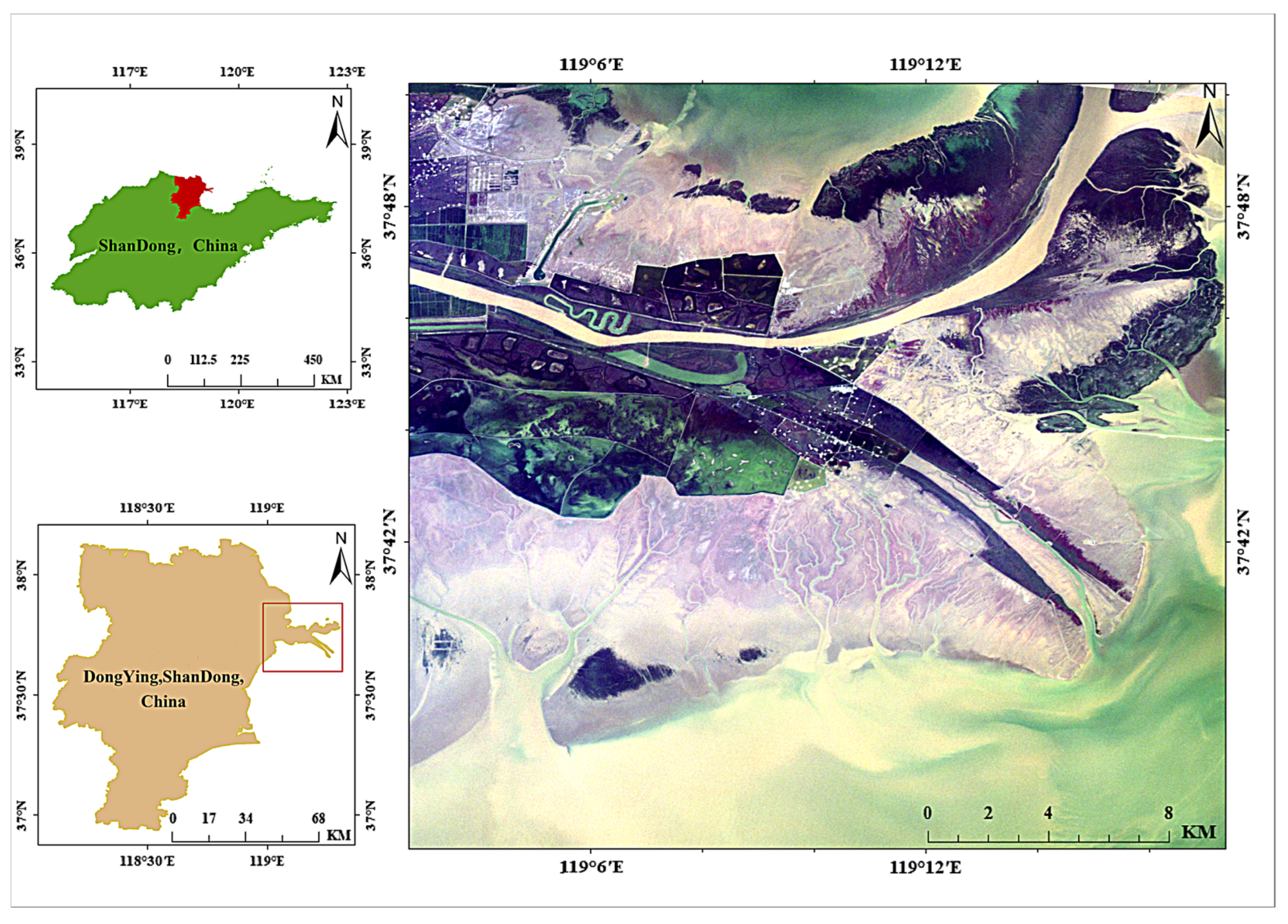
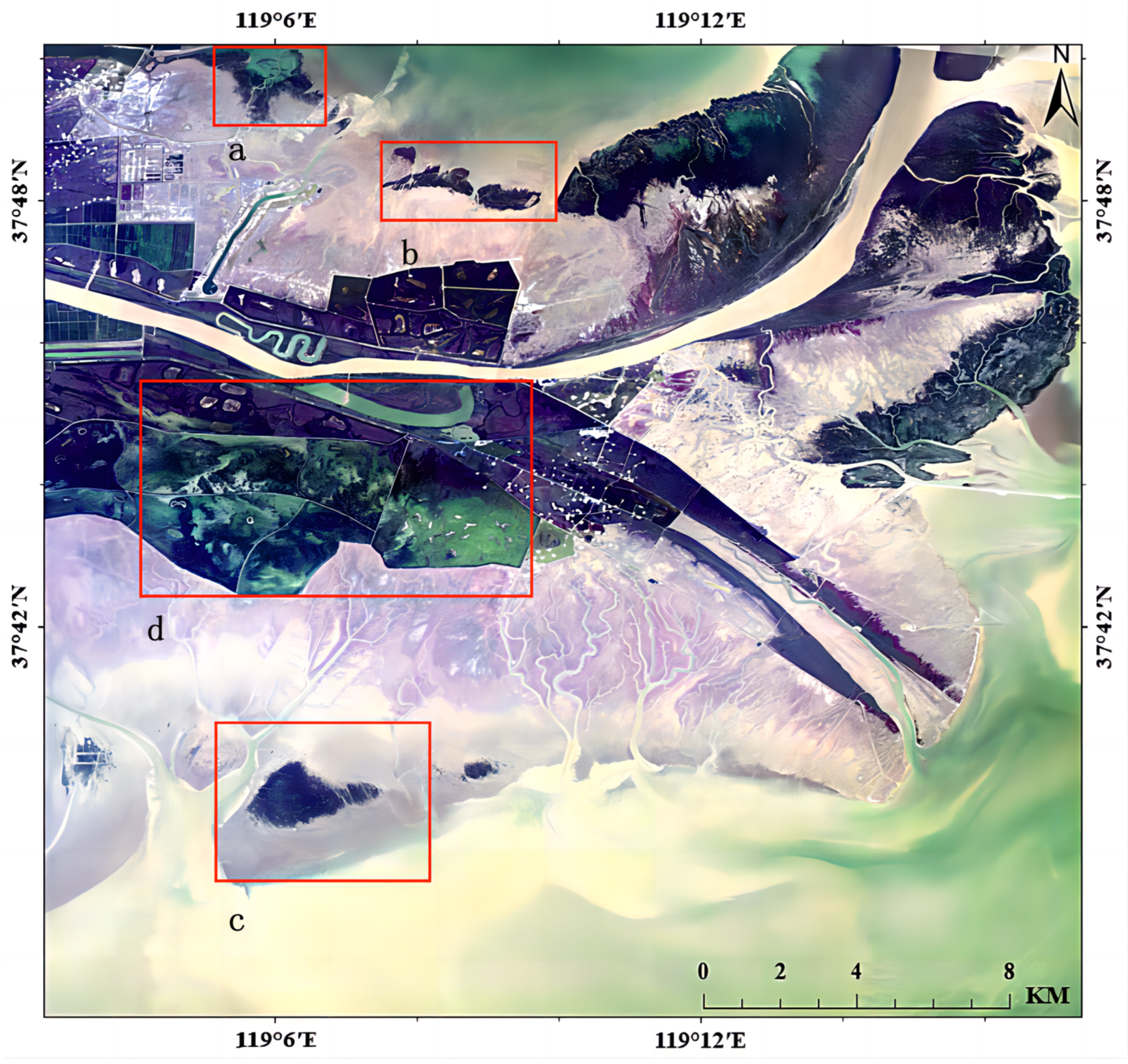
2.1. Overview of the Study Area
2.2. Data Sources and Preprocessing
3. Research Methods
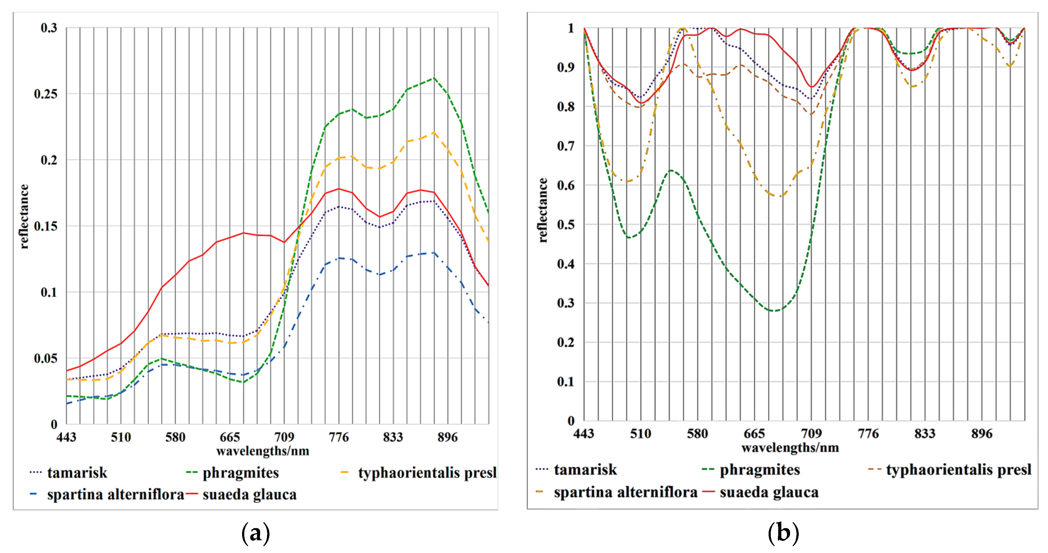
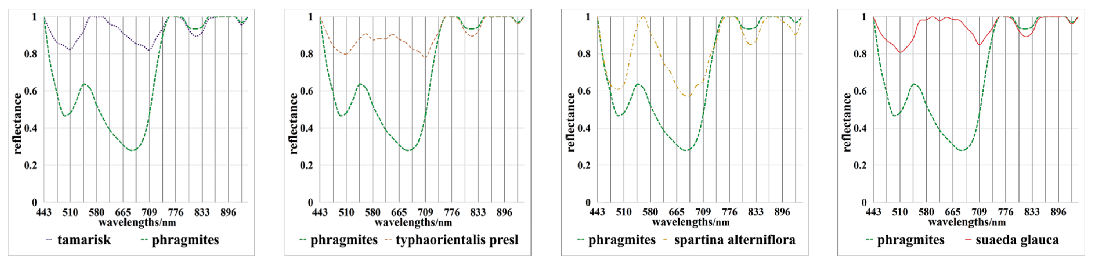
3.1. Continuum Removal
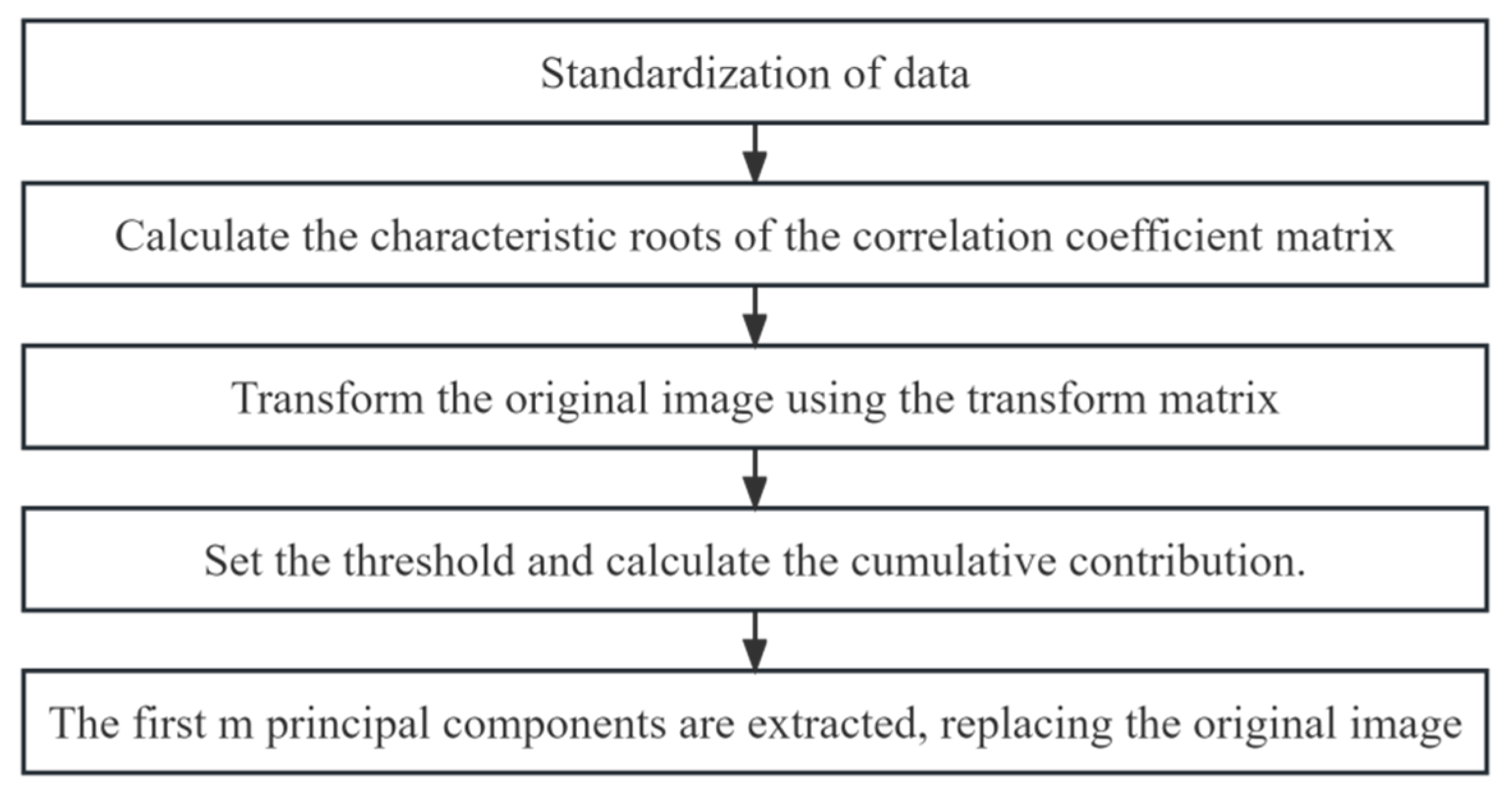
3.2. Principal Component Analysis (PCA)
3.3. Random Forest
3.4. Accuracy Evaluation
3.5. NDVI, NDWI, NDVIre
4. Results and Analysis
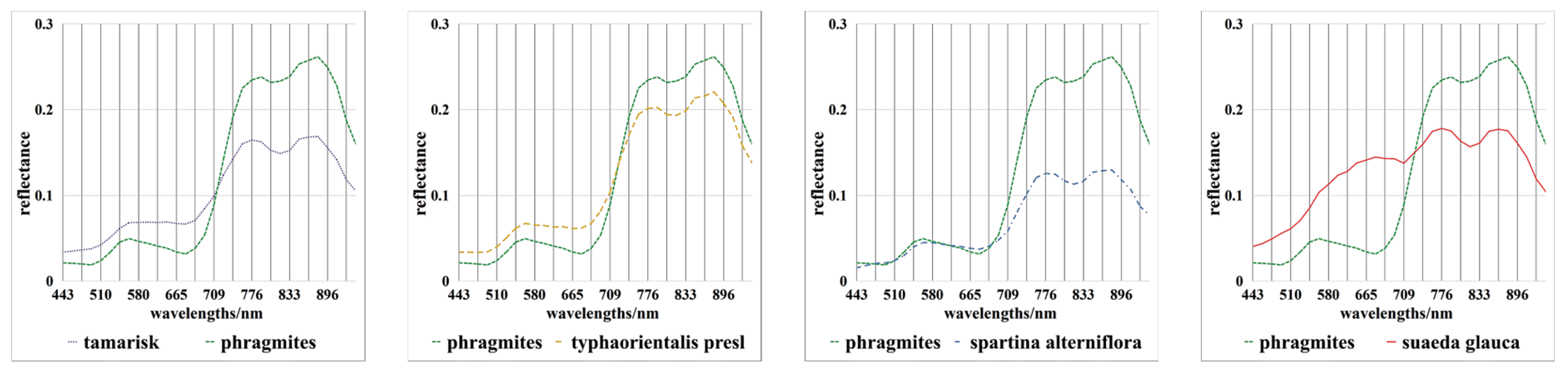
4.1. Characteristic Band Selection Analysis
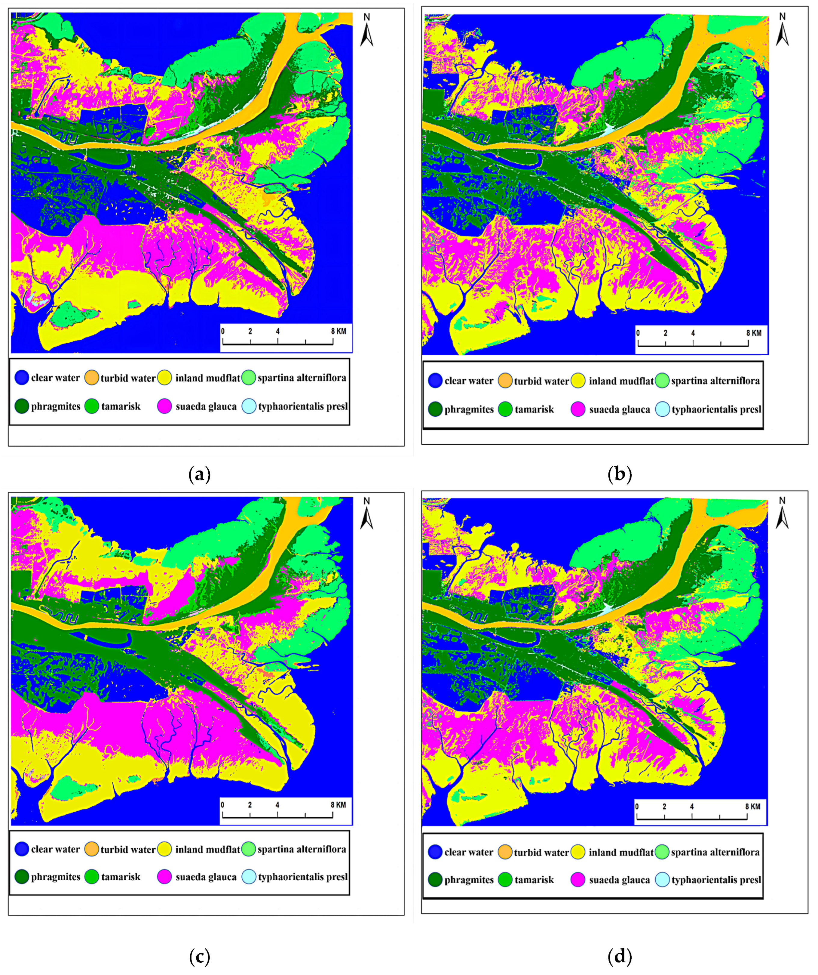
4.2. Vegetation Classification and Accuracy Verification
4.3. Analysis of Vegetation Area Changes
5. Conclusions
Author Contributions
Funding
Institutional Review Board Statement
Data Availability Statement
Conflicts of Interest
References
- Liu, L.; Han, M.; Liu, Y.B.; Pan, B. Spatial distribution of wetland vegetation biomass and its influencing factors in the Yellow River Delta Nature Reserve. J. Ecol. 2017, 37, 4346–4355. [Google Scholar]
- Zhang, C.; Chen, S.; Li, P.; Liu, Q. Current spatiotemporal dynamic remote sensing monitoring of typical wetland vegetation in Yellow Estuary Reserve. J. Oceanogr. 2022, 44, 125–136. [Google Scholar]
- Cui, B.; He, Q.; Gu, B.; Bai, J.; Liu, X. China’s Coastal Wetlands: Understanding Environmental Changes and Human Impacts for Management and Conservation. Wetlands 2016, 36, 1–9. [Google Scholar] [CrossRef]
- Han, M.; Zhang, X.; Liu, L. Progress in Yellow River Delta wetlands. Ecol. Environ. 2006, 872–875. [Google Scholar] [CrossRef]
- Chang, X.; Zeng, H.; Liu, M. Vegetation type, biomass and their relationship with soil environmental factors in the Yellow Sea and Bohai Sea coastal wetlands. J. Ecol. 2018, 37, 3298–3304. [Google Scholar] [CrossRef]
- Mol, J.; Cao, Y.; Hu, Y.; Liu, M.; Xia, D. Object-oriented remote sensing classification of wetland landscape—Take the south bank area of Hangzhou Bay as an example. Wetl. Sci. 2012, 10, 206–213. [Google Scholar] [CrossRef]
- Zomer, R.J.; Trabucco, A.; Ustin, S.L. Building spectral libraries for wetlands land cover classification and hyperspectral remote sensing. J. Environ. Manag. 2007, 90, 2170–2177. [Google Scholar] [CrossRef]
- Chen, Y.; Kuang, R.; Zeng, S. Analysis of typical vegetation identification in Poyang Lake wetland based on hyperspectral data. People Yangtze River 2018, 49, 19–23. [Google Scholar] [CrossRef]
- Huang, J.; Sun, Y. It is suitable for hyperspectral vegetation index screening of 5 plant species in Honghe wetland. Wetl. Sci. 2016, 14, 888–894. [Google Scholar] [CrossRef]
- Zhang, Y.; Na, X.; Zang, S. Fine classification of wetlands based on HJ-1A hyperspectral images. Prog. Geogr. Sci. 2018, 37, 1705–1712. [Google Scholar] [CrossRef]
- Gao, C.; Jiang, X.; Zhen, J.; Wang, J.; Wu, G. Distribution of mangrove species, coupled to WorldView-2 and Zhuhai 1 images. J. Remote Sens. 2022, 26, 1155–1168. [Google Scholar] [CrossRef]
- Bian, F.; Wang, X.; Yang, Z.; Fan, D. Mangrove remote sensing extraction method for hyperspectral data of Zhuhai-1 satellite. Spacecr. Eng. 2021, 30, 182–187. [Google Scholar] [CrossRef]
- Li, R. Progress in hyperspectral forestry. Agric. Sci. Anhui Prov. 2014, 42, 2801–2805. [Google Scholar] [CrossRef]
- Li, C.; Wang, J.; Wu, G.; Li, Q. Classification of agricultural regional plants based on leaf spectral characteristics. J. Shenzhen Univ. 2018, 35, 307–315. [Google Scholar] [CrossRef]
- Liu, P. Research on Plant Classification and State Monitoring Method Based on Hyperspectral Technology. Master’s Thesis, Hangzhou Dianzi University, Hangzhou, China, 2020. [Google Scholar]
- Yang, H.; Du, J.; Ruan, P.; Zhu, X.; Liu, H.; Wang, Y. Classification method of desert grassland vegetation based on UAV remote sensing and random forest. J. Agric. Mach. 2021, 52, 186–194. [Google Scholar] [CrossRef]
- Xiao, Y.; Zhou, D.; Gong, H.; Zhao, W. Global sensitivity analysis of canopy reflection spectrum on physicochemical parameters of vegetation. J. Remote Sens. 2015, 19, 368–374. [Google Scholar] [CrossRef]
- Ma, X.; Wang, A.; Fu, S.; Yue, X.; Qiu, D.; Sun, L.; Wang, F.; Cui, B. Invasive ecological effect of the Yellow estuary on Zostera japonica. Environ. Ecol. 2020, 2, 65–71. [Google Scholar]
- Sun, D.-B.; Li, Y.-Z.; Yu, J.-B.; Yang, J.-S.; Du, Z.-H.; Sun, D.-D.; Ling, Y.; Ma, Y.-Q.; Zhou, D.; Wang, X.-H.; et al. Spatial distribution of soil nutrient elements and their ecological stoichiometry under different vegetation types in the Yellow River Delta wetland. Environ. Sci. 2022, 43, 3241–3252. [Google Scholar] [CrossRef]
- Zou, Y.; Li, X.; Zhang, X.; Ling, Y.; Li, Y.; Wang, X.; Yang, J.; Guan, B.; Ma, Y.; Song, X. Composition and Structure of Emerging Wetland Plant Communities in the Yellow River Estuary. J. Ecol. 2023, 1–10. Available online: http://kns.cnki.net/kcms/detail/21.1148.Q.20230907.1250.012.html (accessed on 5 November 2023).
- Ba, Q.; Wu, Z.; Zhang, S.; Wu, X.; Wang, H.; Bi, N. The spatial and temporal changes of vegetation in the Yellow Estuary wetland and its influencing factors. J. Ocean. Univ. China (Nat. Sci. Ed.) 2022, 52, 81–94. [Google Scholar] [CrossRef]
- Dong, Y.; Dong, M.; Shan, Y. Tree species identification based on hyperspectral remote sensing. J. N. China Univ. Sci. Technol. 2020, 42, 11–16. [Google Scholar] [CrossRef]
- Wang, Z.; Liu, S.; Peng, H.; Yang, Q. Hyperspectral characteristics of common tree species in Guizhou province based on envelope removal. Mt. Agric. Biol. J. 2020, 39, 15–22. [Google Scholar] [CrossRef]
- Wang, T.; Yu, C.; Zhang, N.; Wang, F.; Bai, T. Based on deenvelope and continuous projection algorithm. Agric. Res. Arid Areas 2019, 37, 193–199+217. [Google Scholar] [CrossRef]
- Song, H.; Chen, G.; Yang, W. Hyperspectral remote-sensing image classification based on PCA. Surv. Mapp. Eng. 2017, 26, 17–20+26. [Google Scholar] [CrossRef]
- Dou, S.; Chen, Z.; Xu, Y.; Zheng, H.; Miao, L.; Song, Y. Hyperspectral image classification based on multi-feature fusion and a canonical dimensionality reduction approach. Mapp. Bull. 2022, 32–36+50. [Google Scholar] [CrossRef]
- Tian, Y.; Zhao, C.; Ji, Y. Application of principal component analysis in dimension reduction of hyperspectral remote sensing images. J. Nat. Sci. Harbin Norm. Univ. 2007, 58–60. [Google Scholar]
- Yang, Y.; Liu, R.; Cao, L.; Yang, M.; Chen, J. Land use information extraction of Zhuhai 1 based on random forest algorithm. Explor. Technol. 2021, 43, 818–824. [Google Scholar] [CrossRef]
- Liu, Y.; Han, Z.; Li, R. Study on vegetation information extraction from tidal flats based on principal component analysis and vegetation index. Remote Sens. Inf. 2010, 45–50. [Google Scholar] [CrossRef]
- Zhang, Y.; Ren, H. Remote sensing extraction of GF-6 images integrating feature optimization and random forest algorithm. J. Remote Sens. 2023, 27, 2153–2164. [Google Scholar] [CrossRef]


| Botanical Name | Latin Name | Subjects | Field Survey Photos |
|---|---|---|---|
| Suaeda glauca | Suaeda glauca(Bunge) Bunge | Chenopodiaceae |  |
| Tamarisk | Tamarix chinensis Lour | Tamarixaceae | 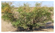 |
| Spartina alterniflora | Spartina alternifloraLoisel | Poaceae |  |
| Typha orientalis Presl | Typha orientalis Presl | Typha orientalis | 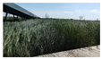 |
| Phragmites | Phragmites australis (Cav.) Trin. ex Steu | Poaceae | 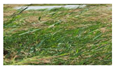 |
| Satellite | Treatment Level | Imaging Time | Number of Bands | Spectral Range | Spectral Resolution | Spatial Resolution |
|---|---|---|---|---|---|---|
| OHS-2C | L1B | 18 September 2020 | 32 | 400~1000 nm | 2.5 nm | 10 m |
| OHS-2C | L1B | 18 September 2020 | 32 | 400~1000 nm | 2.5 nm | 10 m |
| OHS-3B | L1B | 24 July 2022 | 32 | 400~1000 nm | 2.5 nm | 10 m |
| OHS-3B | L1B | 24 July 2022 | 32 | 400~1000 nm | 2.5 nm | 10 m |
| Phragmites | Suaeda Glauca | Tamarisk | Typha Orientalis Presl | Spartina Alterniflora | |
|---|---|---|---|---|---|
| Phragmites |  | 466~709 | 466~730 | 466~700, 806~833 | 490~700, 806~833 |
| Suaeda glauca | 443~686, 746~940 |  | 510~560, 620~709 | 560~730 | 443~531, 580~746, 820~850, 896~940 |
| Tamarisk | 490~686, 746~940 | 560~709 |  | 490~730 | 443~550, 580~730, 806~833 |
| Typha orientalis Presl | 490~686, 760~896 | 560~709, 760~926 | 760~940 |  | 443~580, 620~746, 820~850, 896~926 |
| Spartina alterniflora | 746~940 | 510~896 | 510~686, 746~896 | 746~926 |  |
| Characteristic Variable | Short Title | Description of Features |
|---|---|---|
| Spectral features | Band | B2–B17, B23–B25 |
| Vegetation index | NDVI | (B27–B13)/(B27 + B13) |
| Water index | NDWI | (B27–B13)/(B27 + B13) |
| Red edge index | NDVIred1 | (B27–B15)/(B27 + B15) |
| NDVIred2 | (B27–B16)/(B27 + B16) | |
| NDVIred3 | (B27–B17)/(B27 + B17) | |
| NDVIred4 | (B27–B18)/(B27 + B18) | |
| NDVIred5 | (B27–B19)/(B27 + B19) |
| Characterization Schemes | Combination of Highest Separating Features | Average JM Distance |
|---|---|---|
| Scheme 1 | Band + NDVI + NDWI | 1.6040 |
| Scheme 2 | Band + NDVIred3 | 1.7162 |
| Scheme 3 | Band + NDVI + NDWI + NDVIred3 | 1.8178 |
| Classification | 2020 | 2022 | ||||||||||
|---|---|---|---|---|---|---|---|---|---|---|---|---|
| RF | SVM | MLE | RF | SVM | MLE | |||||||
| PA/% | UA/% | PA/% | UA/% | PA/% | UA/% | PA/% | UA/% | PA/% | UA/% | PA/% | UA/% | |
| Phragmites | 82.00 | 79.35 | 81.33 | 78.21 | 76.00 | 73.08 | 83.33 | 89.29 | 78.67 | 83.10 | 76.00 | 73.08 |
| Suaeda glauca | 78.67 | 83.10 | 80.00 | 82.19 | 74.67 | 76.71 | 80.67 | 80.13 | 76.00 | 78.62 | 74.67 | 76.71 |
| Typha orientalis Presl | 83.33 | 73.53 | 73.33 | 66.67 | 67.33 | 61.21 | 78.00 | 83.57 | 73.33 | 72.85 | 67.33 | 61.21 |
| Tamarix | 79.33 | 79.33 | 78.00 | 78.52 | 78.00 | 78.52 | 82.67 | 77.02 | 80.00 | 78.43 | 72.67 | 73.15 |
| Spartina alterniflora | 85.33 | 85.91 | 84.67 | 83.01 | 70.00 | 68.63 | 86.67 | 82.28 | 84.67 | 84.11 | 70.00 | 68.63 |
| Inland mudflat | 90.00 | 90.00 | 80.00 | 83.92 | 80.00 | 83.92 | 85.33 | 80.00 | 82.00 | 72.35 | 73.33 | 76.92 |
| Clear water | 94.00 | 100.00 | 96.67 | 100.00 | 96.67 | 100.00 | 99.33 | 100.00 | 97.33 | 100.00 | 96.67 | 100.00 |
| Turbid water | 95.33 | 100.00 | 95.33 | 100.00 | 95.33 | 100.00 | 94.00 | 100.00 | 94.67 | 100.00 | 95.33 | 100.00 |
| Overall accuracy | 85.92 | 83.67 | 79.75 | 86.25 | 83.33 | 78.25 | ||||||
| Kappa coefficient | 0.84 | 0.81 | 0.76 | 0.84 | 0.809 | 0.75 | ||||||
| 2020 Raw Images | 2022 Raw Images | Classification Results for 2020 | Classification Results for 2022 | Major Changes in Vegetation | |
|---|---|---|---|---|---|
| a | 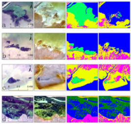 | Spartina alterniflora | |||
| b | Spartina alterniflora | ||||
| c | Spartina alterniflora, Suaeda glauca | ||||
| d | Phragmites | ||||
Disclaimer/Publisher’s Note: The statements, opinions and data contained in all publications are solely those of the individual author(s) and contributor(s) and not of MDPI and/or the editor(s). MDPI and/or the editor(s) disclaim responsibility for any injury to people or property resulting from any ideas, methods, instructions or products referred to in the content. |
© 2023 by the authors. Licensee MDPI, Basel, Switzerland. This article is an open access article distributed under the terms and conditions of the Creative Commons Attribution (CC BY) license (https://creativecommons.org/licenses/by/4.0/).
Share and Cite
Jiang, J.; Tian, H.; Fu, P.; Meng, F.; Tong, H. Spatial and Temporal Changes of Typical Vegetation in the Yellow River Delta Based on Zhuhai-1 Hyperspectral Data. Appl. Sci. 2023, 13, 12614. https://doi.org/10.3390/app132312614
Jiang J, Tian H, Fu P, Meng F, Tong H. Spatial and Temporal Changes of Typical Vegetation in the Yellow River Delta Based on Zhuhai-1 Hyperspectral Data. Applied Sciences. 2023; 13(23):12614. https://doi.org/10.3390/app132312614
Chicago/Turabian StyleJiang, Junyi, Hao Tian, Pingjie Fu, Fei Meng, and Hongju Tong. 2023. "Spatial and Temporal Changes of Typical Vegetation in the Yellow River Delta Based on Zhuhai-1 Hyperspectral Data" Applied Sciences 13, no. 23: 12614. https://doi.org/10.3390/app132312614
APA StyleJiang, J., Tian, H., Fu, P., Meng, F., & Tong, H. (2023). Spatial and Temporal Changes of Typical Vegetation in the Yellow River Delta Based on Zhuhai-1 Hyperspectral Data. Applied Sciences, 13(23), 12614. https://doi.org/10.3390/app132312614