Characterizing the Vibration Responses of Flexible Workpieces during the Turning Process for Quality Control

Featured Application

This study represents a breakthrough in the engineering of turning processes for manufacturing. By examining dynamic properties and vibration response during turning, it provides key insights for real-time machining system monitoring. The findings can improve surface quality and stability, particularly for slender, flexible shafts. Industries such as automotive, aerospace, and heavy equipment manufacturing can leverage these insights to optimize machine performance, reduce downtime, and boost productivity. This marks a significant stride towards more efficient manufacturing.

Abstract

The chatter that occurs during the turning operation, especially when cutting a slender and flexible shaft, determines the surface quality of the workpiece and the stability of the machining system. However, when building a dynamic model of a slender workpiece with a chuck and tailstock, it is generally regarded as a cantilever or simply supported beam, without consideration of the axial force and supported stiffness effect. In this work, a dynamic model for thin and flexible workpieces with different clamping boundary conditions was first built. Then, a finite element analysis (FEA) was used to study the influence of the axial force and supporting stiffness on the mode frequencies of the workpiece. A further analysis found that the relationship between support stiffness, axial force, and the dynamic response of the workpiece is nonlinear and far more complex than that of the simply supported beam model. The clamping force directly influenced the magnitude of the vibration response with the decrease of shaft stiffness during the turning process. These results were verified experimentally by measuring the vibrational response of slender shafts with different clamping modes using an on-rotor sensing (ORS) system. It proved that the proposed model shows advantages for the identification of dynamic vibration and quality control when machining slender workpieces.

1. Introduction

Turning is a common manufacturing process that is used to create revolved parts by eliminating unwanted materials. Vibration occurs during the cutting processes in rotational machinery, particularly in the turning of slender workpieces. Many studies have been conducted to measure its dynamic characteristics, reduce its magnitude, and improve the quality and stability of machining [1,2], in particular, by chatter avoidance [3,4]. Chen et al. [5] analysed the stability of the system during the cutting of a flexible workpiece supported by a tailstock; they studied the effect of the static deformation of the workpiece rather than the dynamics of the tool alone. Liu et al. [6] investigated the dynamic characteristics of a tool-holder by simplifying it as a cantilever beam and formulated the natural frequency based on the Euler–Bernoulli beam theory. Chanda et al. [7] conducted a nonlinear dynamic analysis of a flexible workpiece and tool, obtaining the fundamental frequencies of a shell model of a thin cylindrical workpiece via finite element analysis (FEA). Lu et al. [8] developed a model to predict chatter during the turning of slender workpieces. They considered the changes in the cutting position while the workpiece was supported by a tailstock; dynamic behaviour during chatter could be inferred from their model by considering linear stability and stiffness distribution. Tang et al. [9] optimised process parameters such as cutting forces, cut depth, feed, and tool life for two-tool parallel turning but did not provide a theoretical dynamic model. All these stability studies of turning focused on the interaction of the workpiece and tool; they usually also simplified the tailstock-supported workpiece by representing it as a cantilever beam or as a simple supported beam, which deteriorates the estimation accuracy of the workpiece frequency and modal stiffness of the turning system.

However, a slender workpiece located in a turning dynamic system (see Figure 1) is generally regarded as a combination of a cantilever and a simply supported beam, shown in Figure 2a. The mathematical models developed in these studies usually assumed certain ideal boundary conditions [10]: supported beams were treated as pinned–pinned, fixed–free (cantilever), fixed–pinned, or fixed–fixed. However, when a workpiece is clamped into a machining system, the loss of stiffness lowers the natural frequency of the first bending mode of the shaft compared to what it would be with any of these ideal boundary conditions [11]. This dramatically affects the dynamic response, especially for the resonant vibration response during machining process. Beri B et al. [12] constructed a one degree-of-freedom mechanical model considering the varying modal stiffness of the workpiece and improved the stability properties of turning a slender workpiece by applicating a compressive force at the tailstock. Research has been conducted to evaluate the dynamic responses of the beam model with different boundary conditions under moving loads [13]. Some theoretical and experimental studies of parallel turning stability have represented the tools by springs and damping elements [14]. For example, Saffury and Altus [15] studied the forced harmonic motion of a non-uniform beam with dynamic vibration analytically, using the functional perturbation method [16]. This method can be applied to a cutting tool holder by optimising the real part of the frequency response function to enhance its ability to resist regenerative chatter. The natural frequencies and modes in the turning-point frequency range under various boundary conditions have been studied in this way for shells of revolution [17]. Sun Y et al. established a two-dimensional (2D) dynamic model of the tool and part considering flexible boundary constraints [18]. They found that the dynamics and stability of a slender workpiece were affected by the connection stiffness of boundary constraints (chuck, tool nose, and tailstock). Additionally, vibration is a contributing factor to many problems, such as workpiece surface quality, noise, tool wear, and chatter in machinery. Therefore, it is urgent to establish a more accurate dynamic response model, which comprehensively takes into account the flexible boundary conditions and forces, especially for a slender workpiece.

The finite element method (FEM) is an effective and widely used numerical method that yields results very close to the experimental values [19,20,21,22]. Shang et al. [23] presented an enriched finite element formulation (more efficient than conventional FEA) for analysing the dynamics of one-dimensional bars and Euler–Bernoulli beams. Saju and Deepak designed an FEA system using MATLAB to conduct modal analysis of cantilever beams [24]. In their analysis of the effects of various parameters on diametral error during turning with a follower rest, the authors of [25] used a beam element to create a mesh for a slender bar. This approach yielded both a stiffness matrix and a mass matrix. However, they simplified the model by representing the chuck, tailstock, acting point, and follower rest as four nodes, treating them as hinges.

The remainder of this paper is organised as follows: Section 2 presents the dynamic model of a flexible workpiece with a tailstock. Section 3 establishes the numerical matrix of the dynamic model using FEA. Section 4 presents the effects of the axial force and supporting stiffness on the natural frequency of the shaft. Section 5 presents the experimental results obtained from a general lathe and shows that they are consistent with the theoretical model. Finally, Section 6 describes our conclusions.

2. Dynamic Model of Turning a Slender Shaft

When a slender shaft is turned, one end is fixed to the lathe with a three-jaw chuck, the other end is usually supported by a tailstock centre to increase the stability of the processing and ensure the surface quality of the turning shaft [26,27] (see Figure 1).

A dynamic model for the slender shaft with one end fixed by the three-jaw chuck and the other end pinned by the tailstock, shown in Figure 1, was developed in this study by setting the end pinned by the tailstock as a flexible boundary, shown in Figure 2b. The three-jaw chuck, which limits the deflection and angle of the shaft, is approximated as a fixed support. The tailstock typically has two pairs of thrust bearings to withstand the axial force from the workpiece, as well as a radial bearing to support transverse loads; the thrust bearing enables the apex to provide a preloaded axial force [28] to the slender shaft, whereas the radial bearing provides lateral support. Therefore, the force on the pinned end is approximated as an axial force P and the bearing support is assumed as a spring that provides the model with external stiffness support $\mathit{K}\mathit{t}$ in the Y direction.

Since this model addresses the turning process of slender shafts, axial vibration, shear stress, and rotational inertia are not considered in this simplified model, therefore, the slender shafts are assumed to be continuous Eulerian–Bernoulli beam models [23]. In turning a shaft with high flexibility, it is common to assume the tool as rigid, and the workpiece as a single degree of freedom (SDOF) model, shown in Figure 2b. For a flexible workpiece, the modal stiffness of the workpiece is significantly larger in the axial direction than that in the bending direction. Hence, the vibration of transverse bending is the most significant dynamic response [29]. Thus, the workpiece vibration of transverse bending in the X direction is established as follows:

$$M(x)\frac{{\partial }^{2}w\left(x,t\right)}{\partial t^2}+\frac{{\partial }^2}{\partial x^2}\left[EI\left(x\right)\frac{{\partial }^{2}w\left(x,t\right)}{\partial x^2}\right]=F_c\left(x,t\right)+P(l,t)$$

(1)

where $E$ is workpiece modulus of elasticity, $M\left(x\right)$ is the equivalent mass matrix per unit length, and $I\left(x\right)$ is the moment of inertia at point $x$ of the SDOF model. The mass matrix $M$ and the moment of inertia $I\left(x\right)$ are considered as homogenous and constant. For convenience of formulation, the mass $M\left(x\right)$ and moment of inertia $I\left(x\right)$at each node are directly expressed as $M$ and $I$. $w(x,t)$ is the lateral displacement for each point $x$ of workpiece. $P(l,t)$ is the axial force acting at the pinned end at point $l$, for convenience, it is subsequently expressed as $P$. $F_c\left(x,t\right)$ is the cutting force at time $t$ and at point $x$ in the turning system and can be expressed as [30]

$$F_c\left(x,t\right)=k_s(\mathrm{D}\mathrm{O}\mathrm{C}-\mathrm{D}\left(t\right)+\mathrm{D}(t-\mathrm{T}\left)\right)a_p$$

(2)

where $k_s$ is cutting factor, DOC is the depth of cut, $\mathrm{D}\left(t\right),\mathrm{D}(t-\mathrm{T})$ are the current cutting diameter and the workpiece diameter of the previous turning, respectively. $a_p$ is the feed rate. Substituting Equation (2) into Equation (1), Equation (1) is then normalized as

$$\ddot{w\left(x,t\right)}+2{\mathit{\omega }}_{\mathit{n}}\dot{\zeta w\left(x,t\right)}+{\mathit{\omega }}_{\mathit{n}}^{2}w\left(x,t\right)=k_f\left(\mathrm{D}\left(t-\mathrm{T}\right)-\mathrm{D}\left(t\right)\right)+F$$

(3)

where ${\mathit{\omega }}_{\mathit{n}}$ is the natural frequency of the system, $\zeta$ is the damping ratio, ${\mathit{\omega }}_{\mathit{n}}=\sqrt{\frac{k}{m}}, \zeta =\frac{C}{2{\mathit{\omega }}_{\mathit{n}}}$, $F$ is static component of the total cutting force, $F=\frac{-{\mathit{\omega }}_{\mathit{n}}^2{k}_s{a}_{p}DOC}{\mathit{K}}$,${ k}_f\left(\mathrm{D}\left(t-\mathrm{T}\right)-\mathrm{D}\left(t\right)\right)$ is the dynamic exciting force which is determined by the diameter error, i.e., the surface quality of the workpiece, $k_f=\frac{-{\mathit{\omega }}_{\mathit{n}}^2{k}_s{a}_p}{\mathit{K}}$. To determine the main vibration response, the excitation force in Equation (3) consists of significant random factors, such as nonuniformity of material, inhomogeneous heat treatment, and irregular distributions of hard inclusions, as well as the combined coupling of multiple machining system components. Consequently, it induces significant vibration responses around the natural frequency, especial for the first nth order mode of the slender workpiece. Thus, characterizing these modal responses in resonances is the key way to improve the surface quality and stability of the machining system.

3. Finite Element Analysis Considering Support Stiffness and Axial Force

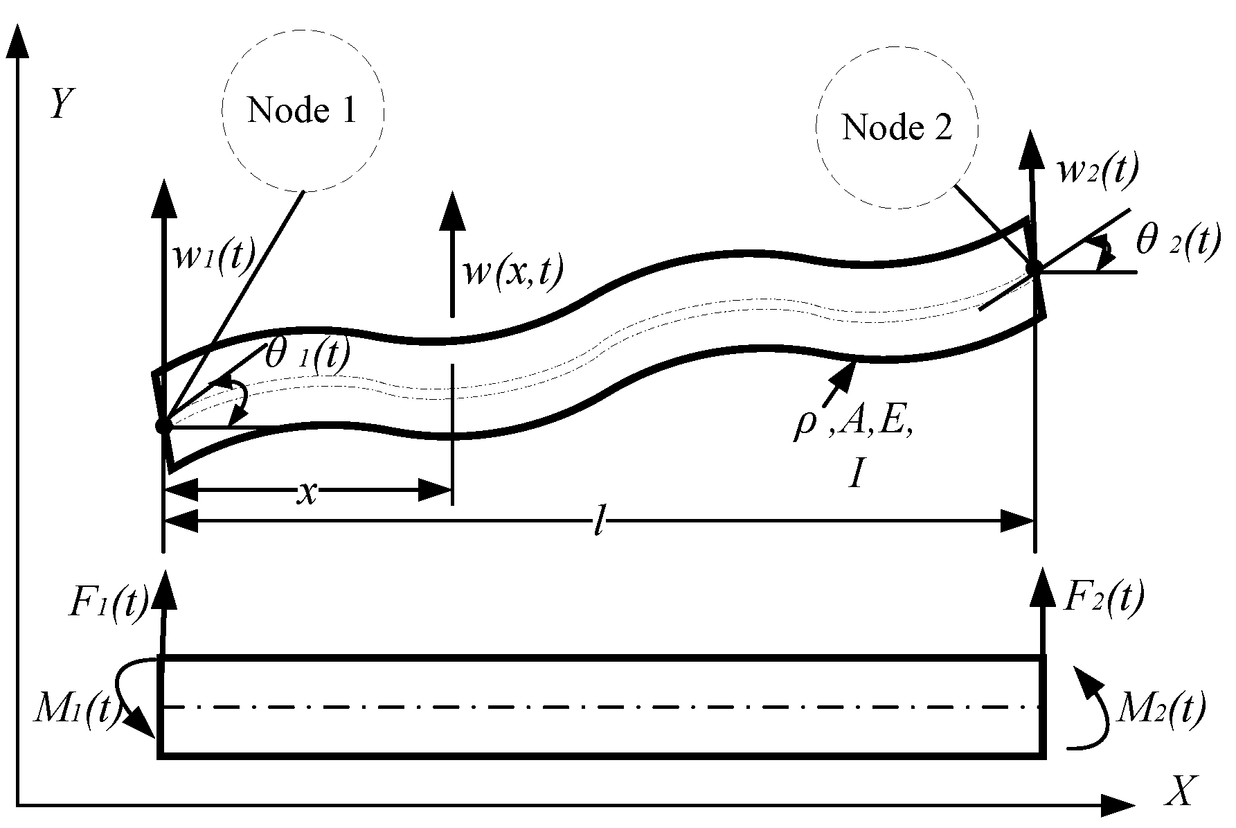
3.1. Stiffness and Mass Matrices of the Shaft Element

FEA, which is widely used to solve structural vibration response [17,18], was used in this study to calculate the natural frequencies of the turning workpiece. In order to solve the modal response of the finite element model, we used MATLAB to build finite elements. In this model, the effects of shear deformation and moment of inertia were ignored because the ratio of the diameter to the length was very small; thus, an Euler–Bernoulli beam element was used [23]. The finite elements are uniformly distributed, and the model converges rapidly through iterative solution. Therefore, only 6 units were set up in this model, each unit had 4 nodes and 4 degrees of freedom.

A typical transversely vibrating element of the shaft is shown in Figure 3. The transverse displacement $w\left(x,t\right)$ of each point in the element is assumed to be consistent with the static deformation curve of the beam along the $x$ direction, obeying the cubic equation [31]

$$w\left(x,t\right)=a\left(t\right)+b\left(t\right)x+c\left(t\right)x^2+d\left(t\right)x^3,$$

(4)

where $a\left(t\right),b\left(t\right),c\left(t\right)\mathrm{a}\mathrm{n}\mathrm{d}d\left(t\right)$ are constants.

The displacement of each node must satisfy the boundary conditions

$$\begin{array}{c}w\left(0,t\right)=w_1\left(t\right),\frac{\partial w}{\partial x}\left(0,t\right)={\theta }_1\left(t\right) ;\\ w\left(l,t\right)=w_2\left(t\right),\frac{\partial w}{\partial x}\left(l,t\right)={\theta }_2\left(t\right).\end{array}$$

(5)

Thus, $a\left(t\right),b\left(t\right),c\left(t\right),d\left(t\right)$ can be determined as

$$\begin{array}{c}a\left(t\right)=w_1\left(t\right),\\ b\left(t\right)={\theta }_1\left(t\right),\\ c\left(t\right)=\frac{1}{l^2}\left(-3w_1\left(t\right)-2{\theta }_1\left(t\right)l+3w_2\left(t\right)-{\theta }_2\left(t\right)l\right),\\ d\left(t\right)=\frac{1}{l^2}\left(2w_1\left(t\right)+{\theta }_1\left(t\right)l-2w_2\left(t\right)+{\theta }_2\left(t\right)l\right).\end{array}$$

(6)

From Equations (6) and Figure 3, $w\left(x,t\right)$ can be expressed as

$$\begin{array}{c}w(x,t)=\left(1-3\frac{x^2}{l^2}+2\frac{x^3}{l^3}\right)w_1\left(t\right)+\left(\frac{x}{l}-2\frac{x^2}{l^2}+\frac{x^3}{l^3}\right)l{\theta }_1\left(t\right)\\ +\left(3\frac{x^2}{l^2}-2\frac{x^3}{l^3}\right)w_2\left(t\right)+\left(-\frac{x^2}{l^2}+\frac{x^3}{l^3}\right)l{\theta }_2\left(t\right),\end{array}$$

(7)

or more conveniently as

$$w\left(x,t\right)={\sum }_{i=1}^4 N_i\left(x\right)\mathit{w}\left(t\right),$$

(8)

where $\mathit{w}\left(t\right)={\left[\begin{array}{c}{w}_1\left(t\right)\hspace{0.25em}\hspace{0.25em}\hspace{0.25em}\hspace{0.25em}{\theta }_1\left(t\right)\hspace{0.25em}\hspace{0.25em}\hspace{0.25em}\hspace{0.25em}{w}_2\left(t\right)\hspace{0.25em}\hspace{0.25em}\hspace{0.25em}\hspace{0.25em}{\theta }_2\left(t\right)\end{array}\right]}^T$. Each element is determined by two nodes, each of which introduces two constraints (for a total of four). Therefore, the shape function $N_i\left(x\right)$ is

$$\begin{array}{c}{N}_1\left(x\right)=1-3{\left(\frac{x}{l}\right)}^2+2{\left(\frac{x}{l}\right)}^3,\\ N_2\left(x\right)=x-2l{\left(\frac{x}{l}\right)}^2+l{\left(\frac{x}{l}\right)}^3,\\ N_3\left(x\right)=3{\left(\frac{x}{l}\right)}^2-2{\left(\frac{x}{l}\right)}^3,\\ N_4\left(x\right)=-l{\left(\frac{x}{l}\right)}^2+l{\left(\frac{x}{l}\right)}^3.\end{array}$$

(9)

The kinetic and deformation energies of each element can be expressed as

$$\begin{array}{c}T(t)=\frac{1}{2}{\int }_0^l \rho A{\left[\frac{\partial w\left(x,t\right)}{\partial t}\right]}^{2}dx=\frac{1}{2}\dot{\mathit{w}}(t{)}^T\mathit{M}\dot{\mathit{w}}\left(t\right),\\ V(t)=\frac{1}{2}{\int }_0^l EI{\left[\frac{{\partial }^{2}w\left(x,t\right)}{\partial x^2}\right]}^{2}dx=\frac{1}{2}\mathit{w}(t{)}^T\mathit{K}\mathit{w}\left(t\right),\end{array}$$

(10)

where $\rho$ is the mass density, $E$ is the Young’s modulus of the material, $I$ is the moment of inertia of the cross section, $A$ is the cross-sectional area, and $\dot{\mathit{w}}\left(t\right)={\left[\begin{array}{c}d{w}_1\left(t\right)/dt\hspace{0.25em}\hspace{0.25em}\hspace{0.25em}\hspace{0.25em}d{\theta }_1\left(t\right)/dt\hspace{0.25em}\hspace{0.25em}\hspace{0.25em}\hspace{0.25em}d{w}_2\left(t\right)/dt\hspace{0.25em}\hspace{0.25em}\hspace{0.25em}\hspace{0.25em}d{\theta }_2\left(t\right)/dt\end{array}\right]}^T$.

After substituting Equation (7) into Equation (10), the mass and stiffness matrices of the transverse vibration of the shaft are obtained by the Rayleigh-Lietz energy method [32]

$$\mathit{M}\mathit{s}=\frac{\rho Al}{420}\left[\begin{array}{cccc}156& 22l& 54& -13l\\ 22l& 4l^2& 13l& -3l^2\\ 54& 13l& 156& -22l\\ -13l& -3l^2& -22l& 4l^2\end{array}\right],$$

(11)

$$\mathit{K}\mathit{s}=\frac{EI}{l^3}\left[\begin{array}{cccc}12& 6l& -12& 6l\\ 6l& 4l^2& -6l& 2l^2\\ -12& -6l& 12& -6l\\ 6l& 2l^2& -6l& 4l^2\end{array}\right].$$

(12)

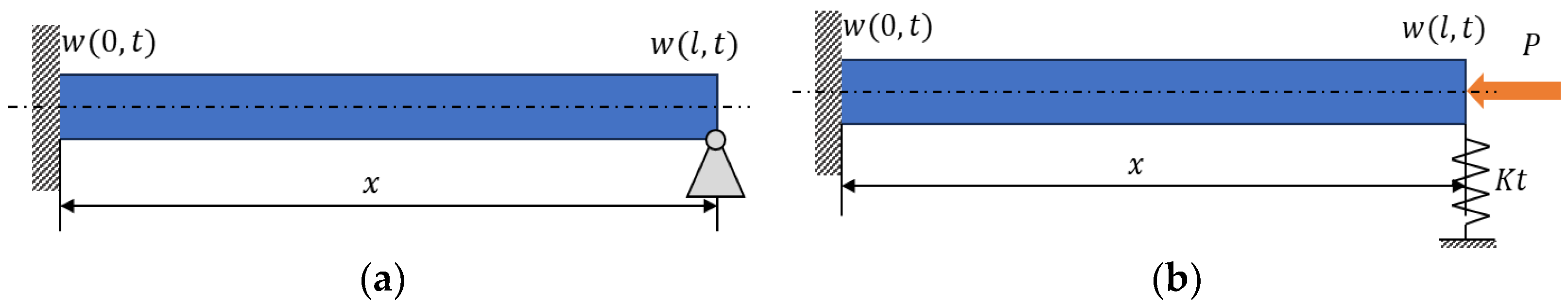
3.2. Support Stiffness of the Tailstock

As shown in Figure 4, an external stiffness support $\mathit{K}\mathit{t}$ exists at the right end of the shaft. From Equation (5), the transverse linear displacement of node 2 at the right end of the shaft is $w_2\left(t\right)=w(l,t)$. Therefore, the deformation energy of the equivalent spring is $\frac{1}{2}kt\cdot w(l,t{)}^2$ and the stiffness support supplied by the spring may be written in matrix form:

$$\mathit{K}\mathit{t}=\left[\begin{array}{cc}\begin{array}{cc}0& 0\\ 0& 0\end{array}& \begin{array}{cc}0& 0\\ 0& 0\end{array}\\ \begin{array}{cc}0& 0\\ 0& 0\end{array}& \begin{array}{cc}kt& 0\\ 0& 0\end{array}\end{array}\right].$$

(13)

The total deformation energy of the shaft element with tailstock is then

$$V(t)=\frac{1}{2}\mathit{w}(t{)}^T\mathit{K}\mathit{s}\cdot \mathit{w}(t)+\frac{1}{2}\mathit{K}\mathit{t}\cdot w_2(t{)}^2,$$

(14)

and the stiffness matrix of the shaft with tailstock support is

$${\mathit{K}}^{\prime }=\mathit{K}\mathit{s}+\mathit{K}\mathit{t}.$$

(15)

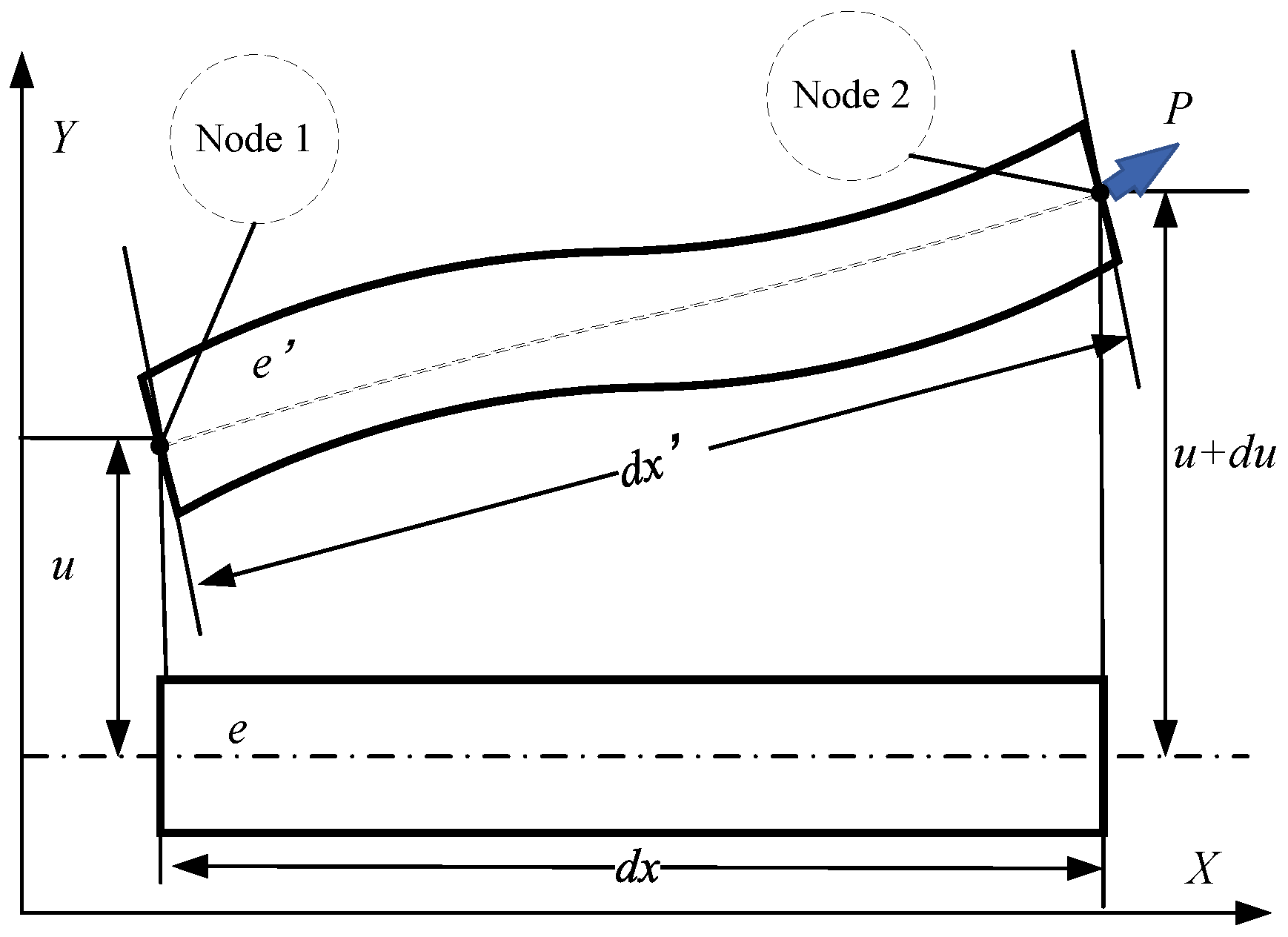
3.3. Influence of Axial Force on Stiffness Matrix

It is assumed that the axial force is not affected by the transverse displacement (Figure 4). Under the action of an axial force, the transverse displacement of the left node 1 is $w_1\left(t\right)=u$, and that of the right node 2 is $w_2\left(t\right)=u+du$. Therefore, the length of the shaft element $e$ after deformation is

$$\begin{array}{c}d{x}^{\prime }=\sqrt{d{x}^2+d{u}^2}\\ =dx\sqrt{1+{\left(\frac{du}{dx}\right)}^2}\approx dx+\frac{1}{2}{\left(\frac{du}{dx}\right)}^2\cdot dx,\end{array}$$

(16)

and the additional strain cause by the axial force on the element is

$${\epsilon }_{x^{\prime }}=\frac{1}{2}{\left(\frac{du}{dx}\right)}^2=\frac{1}{2}{\left(\frac{\partial w(x,t)}{\partial x}\right)}^2,$$

(17)

where $\partial w(x,t)/\partial x$ is the derivative of the transverse displacement curve $w(x,t)$ with respect to $x$ without considering the influence of the axial force.

The additional stress caused by the axial force is denoted ${\sigma }_x$. When the axial force corresponds to the pressure acting on the shaft, it should be negative:

$${\sigma }_x=-P/A.$$

(18)

According to Equations (17) and (18) the additional deformation energy caused by the axial force is

$$\begin{array}{c}{V}_P=\frac{1}{2}\iiint {\sigma }_x{\left(\frac{du}{dx}\right)}^{2}dV=\frac{1}{2}{\int }_0^l P{\left(\frac{du}{dx}\right)}^{2}dx\\ =\frac{1}{2}{\int }_0^l P{\left(\frac{\partial w(x,t)}{\partial x}\right)}^{2}dx=\frac{1}{2}\mathit{w}(\mathit{t}{)}^T\cdot \mathit{K}\mathit{p}\cdot \mathit{w}\left(\mathit{t}\right),\end{array}$$

(19)

where $\mathit{K}\mathit{p}$ denotes an additional stiffness matrix; it may be found by inserting Equation (7) into Equation (19):

$$\mathit{K}\mathit{p}=-\frac{P}{30l}\left[\begin{array}{cccc}36& 3l& -36& 3l\\ 3l& 4l^2& -3l& -l^2\\ -36& -3l& 36& -3l\\ 3l& -l^2& -3l& 4l^2\end{array}\right].$$

(20)

Combing the stiffness matrix of the uniform shaft, the stiffness matrix of the tailstock radial bearing, and the additional stiffness matrix of the shaft under axial force, the total stiffness matrix of the transversely vibrating element of the shaft can be obtained:

$$\mathit{K}=\mathit{K}\mathit{s}+\mathit{K}\mathit{t}+\mathit{K}\mathit{p}.$$

(21)

For an Euler–Bernoulli shaft, the critical axial load of a slender compression bar can be calculated using Euler’s formula:

$$P_{cri}=\frac{{\pi }^{2}EI}{(\mu l{)}^2},$$

(22)

where $\mu$ is the length coefficient of the slender compression bar.

4. Simulation Results Using FEA Method

The main issue in the turning process is the interaction of the lathe system with the bar as the shaft diameter diminishes; this is described by coupled differential equations. It has been proven that using the finite element method to solve these equations produces numerical stiffness values close to the analytical results [17], especially for the first natural frequency.

The key parameters of the shaft in this study are shown in

Table 1. Shaft parameters.

Shaft Material	Initial Diameter	Length	Young’s Modulus E	Mass Density ρ
Q235	22 mm	215 mm	200 GPa	7850 kg m−3

.

4.1. Influence of Tailstock Radial Stiffness on the Shaft’s Mode Frequency

First, we analysed the influence of the tailstock’s radial stiffness on the natural frequency of the shaft using FEA. The results of keeping the diameter of the shaft and the magnitude of the axial force constant and changing $Kt$ are shown in Figure 5. The bearing stiffness had a significant effect on the natural frequency of the shaft. With an increase in the support stiffness, the transverse vibration frequency increased nonlinearly. According to the numerical and experimental results, the natural frequency of the shaft supported by the tailstock was approximately 600 Hz; therefore, the tailstock stiffness was set as $6\times {10}^5 \mathrm{N}/\mathrm{m}$.

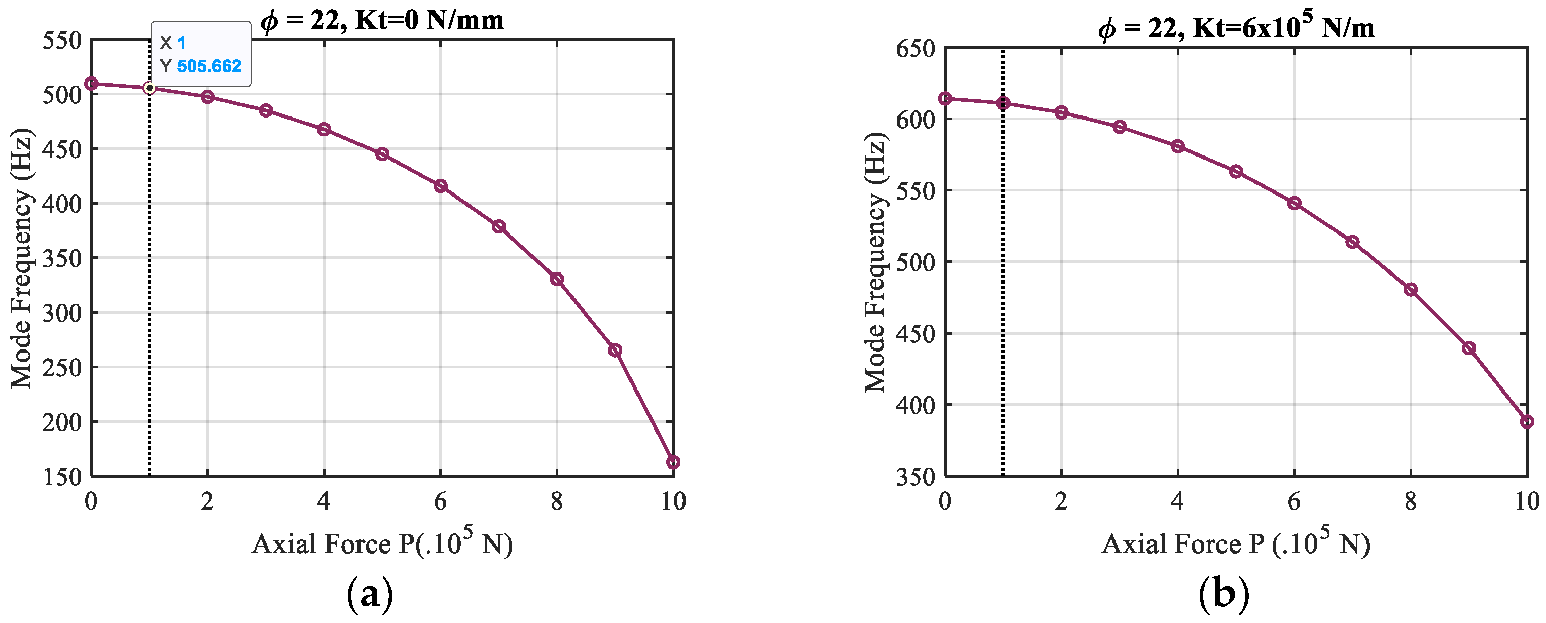
4.2. Influence of Axial Force on Shaft’s Mode Frequency

The results of keeping the shaft diameter $\varnothing$ and the tailstock radial-bearing stiffness $Kt$ constant and changing the axial force $P$ are shown in Figure 6. The natural frequency of the shaft decreased nonlinearly under the action of the axial pressure. According to the numerical and experimental results, the pre-tightening force of the tailstock corresponded to an axial force of $1\times {10}^5 \mathrm{N}$. Therefore, we set $P=1\times {10}^5 \mathrm{N}$.

4.3. Influence of Shaft Diameter on Mode Frequency

During the cutting process, the diameter of the shaft decreases constantly. Therefore, the behaviour of the transverse vibration frequency of the shaft with a decrease in its diameter was analysed for a fixed bearing-support stiffness and axial pressure at the tailstock.

According to Figure 7, when the tailstock support stiffness was $Kt=0 \mathrm{N}/\mathrm{m}$, and the axial pressure was$P={10}^5 \mathrm{N}$, plotting transverse-vibration natural frequency of the shaft against diameter resulted in a curve that was concave downward with positive slope. When the tailstock support stiffness was $Kt={10}^5 \mathrm{N}/\mathrm{m}$ and the axial pressure was $P={10}^5 \mathrm{N}$, the curve was concave upward with a clear minimum between 10 and 12 mm. When the tailstock support stiffness was raised to $Kt=6\times {10}^5 \mathrm{N}/\mathrm{m}$ and the axial pressure was kept the same, the transverse vibration natural frequency of shaft first decreased until the diameter fell to a certain value, then increased rapidly with the diameter decrease; the rate of increase was much higher than the rate of decrease. When the tailstock support stiffness was $Kt={14\times 10}^5 \mathrm{N}/\mathrm{m}$ and the axial pressure was $P={10}^5 \mathrm{N}$, the natural frequency increased with decreasing shaft diameter.

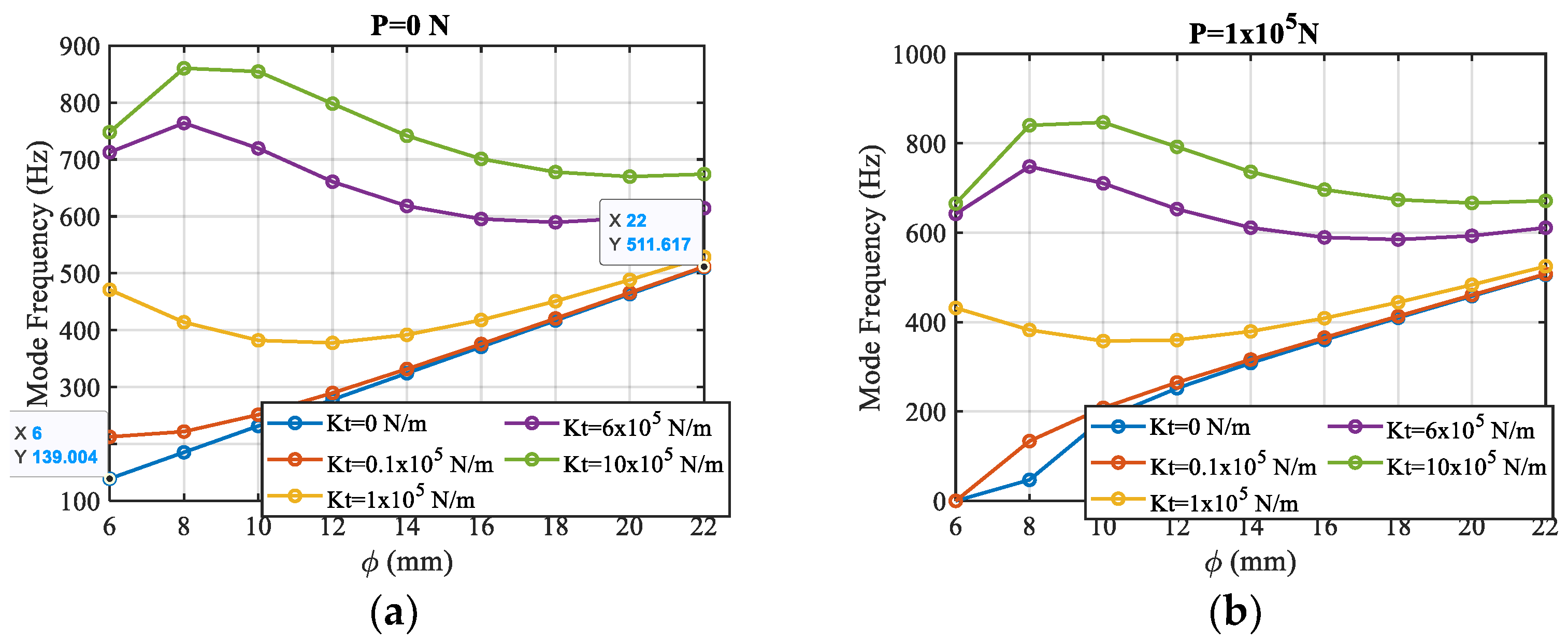
4.4. Influence of Coupling of Shaft Diameter and Tailstock Stiffness

According to the results in Section 4.3, the stiffness determines the natural-frequency curve as the shaft diameter decreases. Therefore, in this section, the variation of the natural frequency with decreasing diameter is analysed for different support stiffnesses and constant axial forces.

As shown in Figure 8, when the support stiffness was very small, the natural frequency of the transverse vibration decreased with a decrease in diameter; this is similar to the results of the cantilever beam model and is consistent with the theoretical results. However, when the support stiffness increased to approximately $1\times {10}^5 \mathrm{N}/\mathrm{m}$, the natural frequency of the shaft first decreased but then increased with decreasing diameter. This is because the mass of the workpiece continued to decrease as the diameter decreased during turning process, and the tailstock support stiffness $Kt$ was much larger compared with the shaft stiffness $Ks$, and tailstock support stiffness influence exceeded that of the shaft itself. Consequently, when the diameter decreased to a certain value, it increased. As the support stiffness continued to increase, its effect became greater than that of the diameter, and the natural frequency exhibited little change as the diameter decreased. The natural frequency decreased sharply only when the diameter reached such a small value that the shaft became unstable, and at the same time, therefore, the ideal boundary conditions of fixed-fixed model [9] is no longer suitable under such large support stiffness.

In conclusion, the support stiffness determines the curve trend of the natural frequency change with the diameter. For $P=0 \mathrm{N}, Kt=0 \mathrm{N}/\mathrm{m}$, the natural frequency is computed as 139.0–511.6 Hz, which is the natural frequency in the cantilever beam model.

4.5. Effect of the Coupling of Shaft Diameter and Axial Force

As can be seen from the above analysis, the support stiffness determines the shape of the curve of the natural frequency versus diameter. Therefore, the effect of the axial force $P$ was analysed by setting the supporting stiffness as Kt = 0, 1 $\times {10}^5$, 6 $\times {10}^5$, and 14 $\times {10}^5$ N/m. In addition, the critical loads for different shaft diameters were calculated using Equation (22). These loads are indicated by red asterisks in Figure 9.

When the support stiffness was constant, the axial force affected the value of the natural frequency but did not change the overall trends in the frequency–diameter curve. Greater axial pressures corresponded to lower natural frequencies, which is consistent with the theoretical analysis. When the axial pressure was greater than the critical load, the calculated value of the natural frequency quickly decreased to zero, and the shaft became unstable.

The second natural frequency was then calculated using the same parameters, as shown in Figure 10. It can be concluded that in most circumstances neither the support stiffness nor axial pressure had any effect. The second-order natural frequency always decreased with decreasing shaft-diameter except when the turning shaft diameter was very small and the axial pressure was greater than the critical load, causing the instability of the shaft.

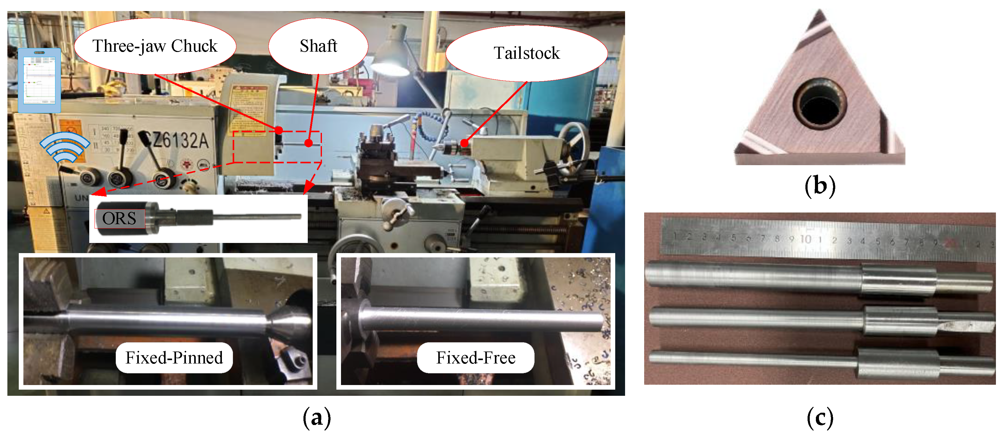
5. Experimental Verification

To verify that the model established in this study provided a realistic description of a lathe processing a slender shaft, an experiment was conducted on a CZ6132A universal machine, shown in Figure 11a. To obtain a more sensitive vibration signal for the cutting parameters and entire rotor system, a novel three-axis wireless on-rotor sensing (ORS) system and a prototype for the turning system were developed, with a sampling rate of 3200 Hz [33]. The installation size of the three-axial acceleration sensor was designed according to the shaft diameter and lathe system. The sensor was installed directly on the shaft rather than on the tool holder or lathe. The vibration signal was collected based on the ORS and directly transmitted to a smartphone through a wireless network [34]. We collected the vibration data once for each layer of workpiece material turned, each sampling time was about 2.5 min with a sampling rate of 3200 Hz. Three different DOCs were set, 0.25 mm, 0.5 mm, and 0.75 mm, and the workpiece was turned at these docs from the original diameter of 22 mm all the way down to a diameter of nearly 12 mm.

The cutting parameters are listed in

Table 2. Cutting parameters.

Cutting Tool	Feed Rate	Spindle Speed	Depth of Cut (mm)	Number of Cuts
Kyocera TNGG 160402R-S PR930	0.05 mm/r	1080 rpm	0.25 mm	12
			0.5 mm	8
			0.75 mm	4

. The material of the cutting tool is coated cemented carbide. The dimensions of the tool, such as the corner radius of 0.2 mm and thickness of 4.76 mm, are shown in Figure 11b. Figure 11c illustrates workpieces of three different diameters.

Two methods of clamping the lathe processing shaft are in common use. In both, one end of the shaft is fixed with a three-jaw chuck. In the first (‘fixed–free’) method, the other end is left free; in the second (‘fixed–pinned’) method, it is supported by a tailstock (Figure 11). When the first method is used, a cantilever beam model can be applied to study the dynamic characteristics directly. There has been little research on the second clamping method; therefore, we studied the dynamic characteristics of transverse vibration with a fixed–pinned shaft model.

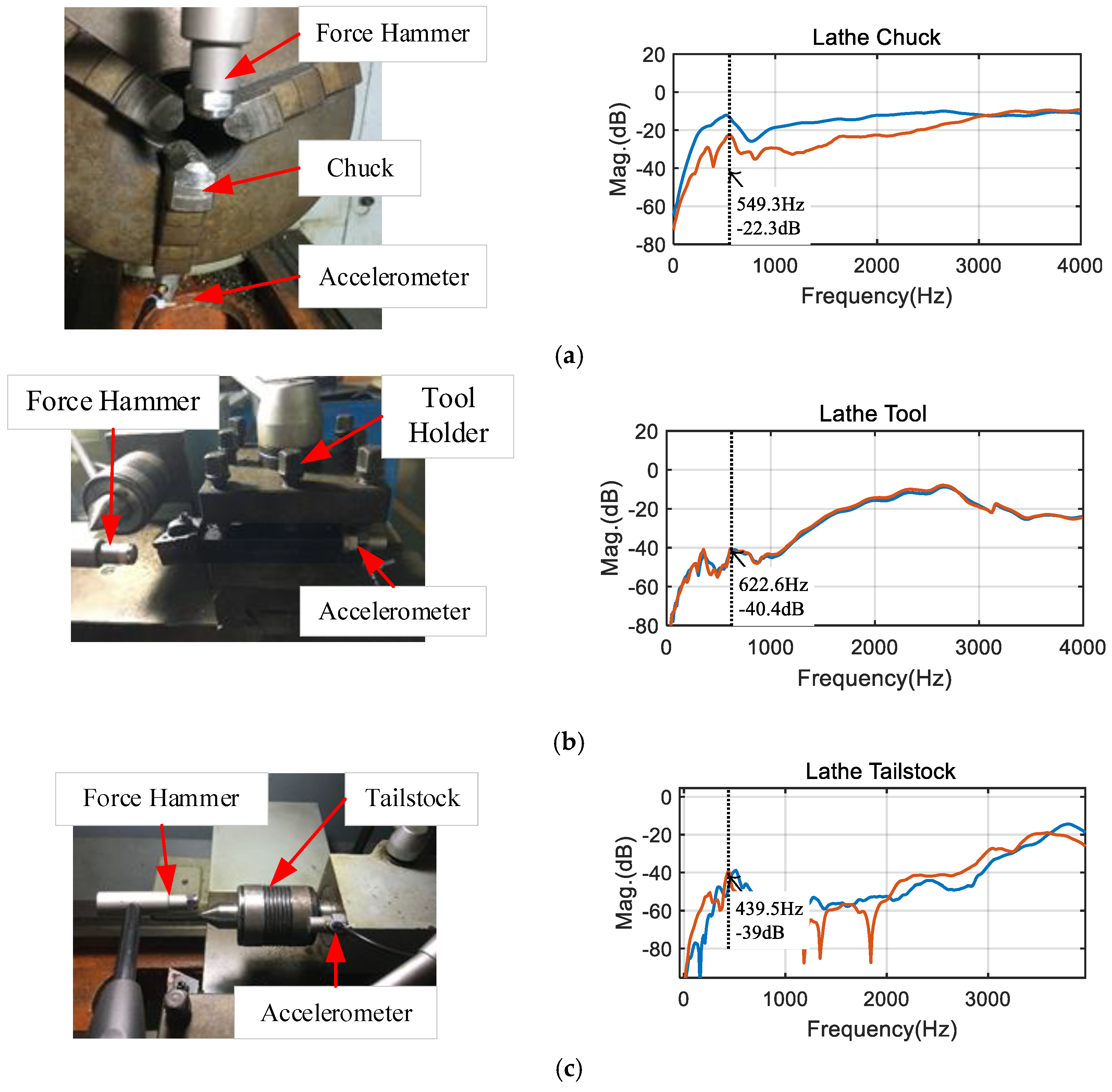
5.1. Frequency Response Function Analysis

To study the influence of the lathe system on the natural frequency of the transverse vibration in the turning process, we first conducted a hammer test to obtain the natural frequencies of the three-jam chuck, tool holder, and tailstock. We mounted a single direction accelerometer, type YMC-122A200, on the chuck, tool holder, and tailstock, respectively, as shown in Figure 12. The vibration signals were recorded with a data acquisition sample frequency of 25 kHz,

To avoid different hammering positions affecting the final measurement results, for each part, we hammered two different positions, each position hammered four times, and then calculated the average value. In Figure 12, the blue and red lines indicate the responses of different hammering positions, respectively. As can be seen, the position has almost no effect on the response results. The peaks of the frequency response plotted in Figure 12 were 549.3, 622.6, and 439.5 Hz, respectively. The measured natural frequencies were typically higher than that of the 2-DOF model with similar overhang length developed in paper [11].

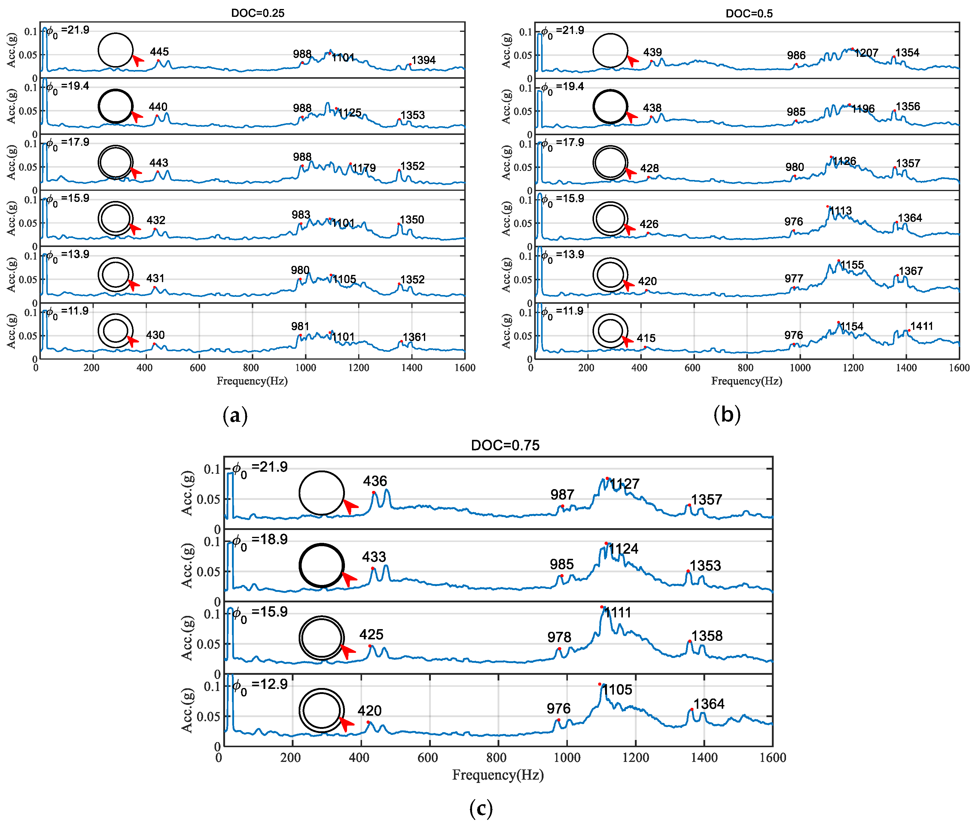
5.2. Analysis of the Transverse Vibration Signal of the Shaft

A CZ6132A lathe was used to process the flexible shafts. The relevant shaft parameters are listed in Table 1. Cutting depth is an important parameter affecting the turning process [26]. Three different cutting depths were used in this experiment: 0.25, 0.5, and 0.75 mm. The transverse vibration signals of the shaft were collected during turning. As turning progressed, the diameter of the shaft decreased continuously according to the cutting depth.

A fast Fourier transform was used to convert the time-domain signal into a frequency-domain signal, which was then smoothed in the frequency domain. The processed signals are shown in Figure 13 and Figure 14, and the red arrow indicated the change in diameter after the workpiece material was turned.

It can be seen that for both clamping modes, there were peaks in the four frequency bands 420–455 Hz, 970–1000 Hz, 1100–1200 Hz, and 1360–1380 Hz, regardless of diameter. It can be inferred that these four frequencies are the natural frequencies of the lathe system (or multiples of them). In particular, the peak value in the 1100–1200 Hz frequency band increased with the cutting depth. It’s well known that cutting depth is related to cutting force [35]: greater cutting depth implies greater cutting force and, thus, a larger vibration peak. Therefore, it can be inferred that the amplitude of the peak value of vibration in the 1100–1200 Hz frequency band is caused by the cutting force. Additionally, this frequency band can be estimated to be twice the frequency of the slender shaft with the effect of the support stiffness from the tool holder, shown in Figure 12b.

The peak value in the 970–1000 Hz frequency band was very stable for both clamping methods; therefore, it is judged to be twice the natural frequency of the three-jaw chuck, which was obtained by the hammer test.

The peak value in the 420–455 Hz frequency band was very stable in the fixed–free clamping mode, but in the fixed–pinned clamping mode it changed significantly as the turning process continued; therefore, it is considered to be the first-order natural frequency of the flexible workpiece with the effect of tailstock supported stiffness.

The location of the peak in the 500–900 Hz frequency band in the fixed–free model was stable (Figure 14) but fluctuated significantly in the fixed–pinned model (Figure 13). The diameter of the shaft was initially 22 mm and decreased continuously during the turning process. In the fixed–pinned model, the frequency corresponding to the peak value of 900 Hz decreased continuously; however, when the diameter was less than 14 mm, the corresponding frequency increased rapidly, and the rate of the increase was much faster than that of the decrease.

According to the numerical results in Figure 9, when $Kt=6\times {10}^5 \mathrm{N}/\mathrm{m}$, the natural frequency first decreased and then increased as the diameter decreased. When the diameter was greater than 15 mm, the natural frequency decreased very slowly, whereas when the diameter was less than 12 mm, the natural frequency increased very quickly as the diameter decreased. The dynamic model of the fixed–pinned system established in this study was thus verified to be correct and consistent with the experimental results.

Figure 15 demonstrated the surface quality of the workpiece with different diameters and clamping modes. As can be seen from the figure, when the diameter of the workpiece at the start of cutting is relatively large, the cutting process was stable and the shaft surface was of high quality, as shown in Figure 15a,b. When the diameter gradually decreased, the cutting process gradually became unstable, and the vibration became larger. In Figure 15c, the surface appeared to have a chattering texture, and in Figure 15d, there were some scratches.

And it can be seen from the final workpiece surface quality in Figure 15c,d that the surface damage manifested itself differently in different clamping modes. However, when the diameter of the slender workpiece is too small, it will lead to the instability of the cutting process, whether it is chattering or skipping, which will eventually affect the surface quality. Therefore, it is very important to study the stability and vibration of the cutting process to control the quality of workpiece being machined.

6. Conclusions

Currently, in the dynamic turning model of a slender workpiece with a chuck and tailstock, it is usually assumed as a simple supported beam model. This simplified rigid constraint boundary, ignoring the influence of the axial preload and support stiffness of the tailstock, inevitably affects the accuracy of the frequency response. Especially for the cutting process of slender flexible shafts, its dynamic response directly determines the machining quality and cutting stability.

To handle these issues, this study innovatively developed a continuous element fixed-pinned model for turning slender workpieces, improving the rigid support at the end of the clamp to be the joint action of the flexible support stiffness and axial force. Moreover, the FEM is used to solve the influence of support stiffness, shaft diameter, and axial force on the modal frequency of slender workpieces. Although the FEM is an approximate numerical solution and cannot accurately estimate the stress between elements, the accuracy of the calculated results is sufficient for slender shaft models with small deformation. It was first found that the supporting stiffness determined the shape of the vibration–diameter curve. Additionally, the axial pressure provided by the tailstock affected the stability of the slender shaft. In particular, when the workpiece diameter was very small, the axial force easily exceeded the critical load, resulting in instability.

A series of modal testing and turning experiments was conducted to verify the proposed model. The vibration response from the ORS effectively explained the natural frequency characteristics of each component of the lathe system and the vibration characteristics during the machining process. The results indicated that the experimental phenomena were in good consistency with the simulation results of the proposed model. The support stiffness of the tailstock and the axial force together determined the dynamic response frequency of the turning process, which is neglected in the classical boundary constraints model.

In conclusion, this study provides valuable insights into the dynamic behaviour of slender and flexible shafts during the turning process, offering a comprehensive investigation through the construction of a dynamic model. It explores how the mode frequencies of workpiece shafts are influenced by various factors, including support stiffness, workpiece diameter, and axial external forces. Notably, we measured the vibration responses during turning process using a novel ORS system. The measurement results of the experiments indicate that the clamping mode of the slender shaft during the cutting process affects the vibration response of the system, thus affecting the surface quality of the workpiece and the stability of the machining system. These findings are essential for the in-process condition monitoring of machining systems, contributing to the optimization of manufacturing processes, surface quality control, and system stability, particularly for those prone to vibration motion.

References

1. Sekar, M.; Srinivas, J.; Kotaiah, K.R.; Yang, S.H. Stability Analysis of Turning Process with Tailstock-Supported Workpiece. Int. J. Adv. Manuf. Technol. 2009, 43, 862–871. [Google Scholar] [CrossRef]
2. Zhou, Y.; Wang, S.; Chen, H.; Zou, J.; Ma, L.; Yin, G. Study on Surface Quality and Subsurface Damage Mechanism of Nickel-Based Single-Crystal Superalloy in Precision Turning. J. Manuf. Process. 2023, 99, 230–242. [Google Scholar] [CrossRef]
3. Stepan, G.; Kiss, A.K.; Ghalamchi, B.; Sopanen, J.; Bachrathy, D. Chatter Avoidance in Cutting Highly Flexible Workpieces. CIRP Ann. Manuf. Technol. 2017, 66, 377–380. [Google Scholar] [CrossRef]
4. Liu, Y.; Liu, Z.; Song, Q.; Wang, B. Development of Constrained Layer Damping Toolholder to Improve Chatter Stability in End Milling. Int. J. Mech. Sci. 2016, 117, 299–308. [Google Scholar] [CrossRef]
5. Chen, C.K.; Tsao, Y.M. A Stability Analysis of Turning a Tailstock Supported Flexible Work-Piece. Int. J. Mach. Tools Manuf. 2006, 46, 18–25. [Google Scholar] [CrossRef]
6. Liu, Y.; Liu, Z.; Song, Q.; Wang, B. Analysis and Implementation of Chatter Frequency Dependent Constrained Layer Damping Tool Holder for Stability Improvement in Turning Process. J. Am. Acad. Dermatol. 2018, 266, 687–695. [Google Scholar] [CrossRef]
7. Chanda, A.; Dwivedy, S.K. Nonlinear Dynamic Analysis of Flexible Workpiece and Tool in Turning Operation with Delay and Internal Resonance. J. Sound Vib. 2018, 434, 358–378. [Google Scholar] [CrossRef]
8. Lu, K.; Lian, Z.; Gu, F.; Liu, H. Model-Based Chatter Stability Prediction and Detection for the Turning of a Flexible Workpiece. Mech. Syst. Signal. Process. 2018, 100, 814–826. [Google Scholar] [CrossRef]
9. Tang, L.; Landers, R.G.; Balakrishnan, S.N. Parallel Turning Process Parameter Optimization Based on a Novel Heuristic Approach. J. Manuf. Sci. Eng. Trans. ASME 2008, 130, 0310021–03100212. [Google Scholar] [CrossRef]
10. Carrer, J.A.M.; Corrêa, R.M.; Mansur, W.J.; Scuciato, R.F. Dynamic Analysis of Continuous Beams by the Boundary Element Method. Eng. Anal. Bound. Elem. 2019, 104, 80–93. [Google Scholar] [CrossRef]
11. Östling, D.; Magnevall, M. Modelling the Dynamics of a Large Damped Boring Bar in a Lathe. Procedia CIRP 2019, 82, 285–289. [Google Scholar] [CrossRef]
12. Beri, B.; Meszaros, G.; Stepan, G. Machining of Slender Workpieces Subjected to Time-Periodic Axial Force: Stability and Chatter Suppression. J. Sound Vib. 2021, 504, 116114. [Google Scholar] [CrossRef]
13. Yekdane, A.; Movahedian, B.; Boroomand, B. An Efficient Time-Space Formulation for Dynamic Transient Analyses: Application to the Beam Assemblies Subjected to Moving Loads and Masses; Elsevier Inc.: Amsterdam, The Netherlands, 2020; ISBN 8415683111. [Google Scholar]
14. Ozturk, E.; Comak, A.; Budak, E. Tuning of Tool Dynamics for Increased Stability of Parallel (Simultaneous) Turning Processes. J. Sound Vib. 2016, 360, 17–30. [Google Scholar] [CrossRef]
15. Saffury, J.; Altus, E. Chatter Resistance of Non-Uniform Turning Bars with Attached Dynamic Absorbers-Analytical Approach. J. Sound Vib. 2010, 329, 2029–2043. [Google Scholar] [CrossRef]
16. Nachum, S.; Altus, E. Natural Frequencies and Mode Shapes of Deterministic and Stochastic Non-Homogeneous Rods and Beams. J. Sound Vib. 2007, 302, 903–924. [Google Scholar] [CrossRef]
17. Zhang, Z.L.; Cheng, C.J. Natural Frequencies and Mode Shapes for Axisymmetric Vibrations of Shells in Turning-Point Range. Int. J. Solids Struct. 2006, 43, 5525–5540. [Google Scholar] [CrossRef]
18. Sun, Y.; Yan, S. Dynamics Identification and Stability Analysis in Turning of Slender Workpieces with Flexible Boundary Constraints. Mech. Syst. Signal. Process. 2022, 177, 109245. [Google Scholar] [CrossRef]
19. Subbarao, R.; Dey, R. Selection of Lathe Spindle Material Based on Static and Dynamic Analyses Using Finite Element Method. Mater. Today Proc. 2019, 22, 1652–1663. [Google Scholar] [CrossRef]
20. Duran, A.; Nalbant, M. Finite Element Analysis of Bending Occurring While Cutting with High Speed Steel Lathe Cutting Tools. Mater. Des. 2005, 26, 549–554. [Google Scholar] [CrossRef]
21. Mahdavinejad, R. Finite Element Analysis of Machine and Workpiece Instability in Turning. Int. J. Mach. Tools Manuf. 2005, 45, 753–760. [Google Scholar] [CrossRef]
22. Jorge, P.C.; Da Costa, A.P.; Simões, F.M.F. Finite Element Dynamic Analysis of Finite Beams on a Bilinear Foundation under a Moving Load. J. Sound Vib. 2015, 346, 328–344. [Google Scholar] [CrossRef]
23. Shang, H.Y.; Machado, R.D.; Abdalla Filho, J.E. Dynamic Analysis of Euler-Bernoulli Beam Problems Using the Generalized Finite Element Method. Comput. Struct. 2016, 173, 109–122. [Google Scholar] [CrossRef]
24. Joseph, S.; Deepak, B.S. Virtual Experimental Modal Analysis of a Cantilever Beam. Int. J. Eng. Res. Technol. 2017, 6, 921–928. [Google Scholar]
25. Jianliang, G.; Rongdi, H. A United Model of Diametral Error in Slender Bar Turning with a Follower Rest. Int. J. Mach. Tools Manuf. 2006, 46, 1002–1012. [Google Scholar] [CrossRef]
26. Li, C.; Li, B.; Gu, L.; Feng, G.; Gu, F.; Ball, A.D. Online Monitoring of a Shaft Turning Process Based on Vibration Signals from On-Rotor Sensor. In Proceedings of the 2020 3rd World Conference on Mechanical Engineering and Intelligent Manufacturing (WCMENIM), Shanghai, China, 4–6 December 2020; pp. 402–407. [Google Scholar] [CrossRef]
27. Segonds, S.; Cohen, G.; Landon, Y.; Monies, F.; Lagarrigue, P. Characterising the Behaviour of Workpieces under the Effect of Tangential Cutting Force during NC Turning: Application to Machining of Slender Workpieces. J. Mater. Process. Technol. 2006, 171, 471–479. [Google Scholar] [CrossRef]
28. Huang, D.; Bian, Y.; Huang, D.; Zhou, A.; Sheng, B. An Ultimate-State-Based-Model for Inelastic Analysis of Intermediate Slenderness PSB Columns under Eccentrically Compressive Load. Constr. Build. Mater. 2015, 94, 306–314. [Google Scholar] [CrossRef]
29. Soleimanimehr, H. Analysis of the Cutting Ratio and Investigating Its Influence on the Workpiece’s Diametrical Error in Ultrasonic-Vibration Assisted Turning. Proc. Inst. Mech. Eng. B J. Eng. Manuf. 2021, 235, 640–649. [Google Scholar] [CrossRef]
30. Li, B.; Gu, L.; Lin, Y.; Zou, Z.; Pang, S.; Lu, K.; Feng, G.; Gu, F.; Ball, A.D. Vibration Monitoring of Turning a Shaft on a Lathe Based on Signals from an On-Rotor Sensor. In Proceedings of the Mechanisms and Machine Science; Springer Science and Business Media B.V.: Berlin/Heidelberg, Germany, 2021; Volume 105, pp. 910–922. [Google Scholar]
31. Rao, S.S. Vibration of Continuous Systems; Wiley: Hoboken, NJ, USA, 2006; ISBN 9786468600. [Google Scholar]
32. Gritsenko, D.; Xu, J.; Paoli, R. Transverse Vibrations of Cantilever Beams: Analytical Solutions with General Steady-State Forcing. Appl. Eng. Sci. 2020, 3, 100017. [Google Scholar] [CrossRef]
33. Li, C.; Zou, Z.; Lu, K.; Wang, H.; Cattley, R.; Ball, A.D. Assessment of a Three-Axis on-Rotor Sensing Performance for Machining Process Monitoring: A Case Study. Sci. Rep. 2022, 12, 16813. [Google Scholar] [CrossRef]
34. Li, C.; Li, B.; Wang, H.; Shi, D.; Gu, F.; Ball, A.D. Tool Wear Monitoring in CNC Milling Process Based on Vibration Signals from an On-Rotor Sensing Method. In International Conference on the Efficiency and Performance Engineering Network; Springer Nature: Cham, Switzerland, 2022; pp. 268–281. [Google Scholar] [CrossRef]
35. Zerti, O.; Yallese, M.A.; Khettabi, R.; Chaoui, K.; Mabrouki, T. Design Optimization for Minimum Technological Parameters When Dry Turning of AISI D3 Steel Using Taguchi Method. Int. J. Adv. Manuf. Technol. 2017, 89, 1915–1934. [Google Scholar] [CrossRef]
Figure 1. Turning a slender shaft fixed to a three-jaw chuck and supported by a tailstock.
Applsci 13 12611 g001
Figure 2. Dynamic model of turning a slender shaft, P = axial force; Kt = spring stiffness. (a) Classical simply supported beam model; (b) fixed-pinned model with flexible boundary.
Applsci 13 12611 g002
Figure 3. Transverse vibration of shaft element.
Applsci 13 12611 g003
Figure 4. Deformation of shaft element under axial force P.
Applsci 13 12611 g004
Figure 5. Influence of tailstock radial bearing stiffness K t on the shaft’s natural frequency for axial force (a) P = 0     N and (b) P = 1 × 10 5     N . = diameter (mm).
Applsci 13 12611 g005
Figure 6. Influence of axial force P on the shaft’s natural frequency for tailstock radial-bearing stiffness (a) K t = 0     N / m and (b) K t = 6 × 10 5     N / m . = diameter (mm).
Applsci 13 12611 g006
Figure 7. Influence of shaft diameter on natural frequency: (a) Tailstock radial bearing stiffness K t = 0     N / m and axial force P = 1 × 10 5     N ; (b) K t = 1 × 10 5     N / m , P = 1 × 10 5     N ; (c) K t = 6 × 10 5     N / m , P = 1 × 10 5     N ; (d) K t = 14 × 10 5     N / m , P = 1 × 10 5     N .
Applsci 13 12611 g007
Figure 8. Influence of coupling of shaft diameter and tailstock stiffness Kt for axial force (a) P = 0     N and (b) P = 1 × 10 5 N .
Applsci 13 12611 g008
Figure 9. First mode frequency for tailstock radial bearing stiffness (a) K t = 0     N / m ; (b) K t = 1 × 10 5   N / m ; (c) K t = 6 × 10 5     N / m ; (d) K t = 14 × 10 5     N / m . Red asterisks show critical axial loads. = diameter; P = axial force.
Applsci 13 12611 g009
Figure 10. Second mode frequency for tailstock radial bearing stiffness (a) K t = 0     N / m ; (b) K t = 1 × 10 5     N / m ; (c) K t = 6 × 10 5     N / m ; (d) K t = 14 × 10 5     N / m . Red asterisks show critical axial loads. = diameter; P = axial force.
Applsci 13 12611 g010
Figure 11. Turning experiment rig, photograph of (a) the turning system, showing the two clamping modes; (b) the tool insert; (c) workpieces of different diameters.
Applsci 13 12611 g011
Figure 12. Natural frequency of the lathe system by hammer test: frequency response functions for (a) chuck; (b) tool holder; (c) tailstock.
Applsci 13 12611 g012
Figure 13. Fixed–pinned on-rotor-sensing vibration signal at depth of cutting (DOC) (a) 0.25 mm; (b) 0.5 mm; (c) 0.75 mm.
Applsci 13 12611 g013
Figure 14. Fixed–free on-rotor-sensing vibration signal at depth of cutting (DOC) (a) 0.25 mm; (b) 0.5 mm; (c) 0.75 mm.
Applsci 13 12611 g014
Figure 15. Workpiece surface quality (a) Φ = 20   m m , fixed-free mode; (b) Φ = 18   m m , fixed-free mode; (c) Φ = 14   m m , fixed-free mode; (d) Φ = 12   m m , fixed–pinned mode.
Applsci 13 12611 g015