Multilevel Regularization Method for Building Outlines Extracted from High-Resolution Remote Sensing Images

Abstract

Extraction of vectorized building outlines from high-resolution remote sensing images is highly useful for various application fields, such as map creation and urban planning. However, this process is often complicated by external factors, such as trees and shadows, which cause issues, such as excessive node redundancy, jagged lines, and unclear corner points. In this study, a multilevel regularization method was designed for building outlines, including the “overall–local–detail” levels. First, overall regularization was performed by combining the minimum bounding rectangle of the building outline with the Hausdorff distance method. Next, based on the convex hull of the building outline and the distribution characteristics of nodes along the outline, the building outline was divided into multiple line chains and classified for local regularization. Finally, the details of the building outline were processed, with the parallel and perpendicular characteristics enhanced to obtain the final regularization results. The experimental results showed that the proposed method effectively enhances the edge representation accuracy of building outlines and significantly improves the accuracy and regularity of building edges. Furthermore, it strengthens the orthogonal characteristics of building outlines, providing more accurate representations of true building outlines.

1. Introduction

Buildings constitute important artificial ground objects that are closely related to human activities. Building outline data have high application value in various fields, such as map creation and updating, disaster analysis, emergency rescue, urban planning, change monitoring, 3D modeling, and population assessment [1]. In recent years, the rapid development of “smart cities,” spatial big data, and artificial intelligence has accelerated the demand for diverse, accurate, and timely building outline data [2]. High-resolution remote sensing images contain rich ground object features, including color, size, shape, texture, and spatial relationships between objects [3]. By employing deep learning and machine learning techniques, building outlines can be extracted rapidly from high-resolution remote sensing images [4,5] and building outline data can be updated in a timely manner. However, high-resolution remote sensing images contain many types of ground objects and face problems such as “same ground objects, different spectra” and “same spectra, different ground objects.” Consequently, accurately identifying the original building outline shapes is difficult, resulting in issues such as omission and misinterpretation [6]. Currently, there are further studies on methods for extracting building outlines from remote sensing images using deep learning and machine learning techniques. However, the extracted outlines are generally in the form of patches and often have problems such as irregular boundaries, unclear inflection points, etc., and high data redundancy. Directly using the extracted initial outline would significantly affect the effectiveness of the use. By contrast, manual repair of the initial outline would significantly reduce work efficiency. To obtain more realistic, accurate, and complete building outlines, studying automatic regularization methods for the outlines is important [7]. Regularization can establish a bridge between “extraction” and “application” and improve the usability of remote sensing images for extracting building outline data. Currently, building outlines are mainly regularized by image morphology, geometric correction, and model matching.

Image morphology methods primarily utilize the texture and shape characteristics of building outlines and regularize building outlines through morphological operations such as erosion, dilation, opening, and closing. Wang et al. [8] first filled the rasterized information of the building outline and then employed morphological algorithms, such as erosion and dilation, to optimize the jagged parts of the outline. Finally, a binary image boundary extraction algorithm was employed to extract the optimized results. Ding et al. [9] initially over-segmented the images through simple linear iterative clustering to obtain super-pixels, and then used seed lines obtained through manual interaction to determine candidate foreground and background images for target buildings. Afterward, a star-shaped shape-constrained image segmentation algorithm was adopted to obtain building patches, and the Harris corner detection algorithm was applied to extract corner points from these patches. The extracted points were grouped, linearly fitted, and rotated to obtain regularized building outlines. Zhou et al. [10] first acquired eigenvectors for segmentation based on the angle and texture characteristics of buildings. Then, the graph-cut method was used to determine candidate building points and, after mathematical morphological processing, to obtain building patches. Finally, the corner points of the buildings were obtained by referring to each building’s main direction and least squares matching template and were then connected to yield the building outline information. Although image morphology methods improve the accuracy and speed of image processing during extraction, they may introduce problems such as node distortion, data redundancy, and endpoint contraction.

Geometric correction methods primarily optimize building outlines using geometric features, such as the direction, angle, and orthogonality of the straight lines constituting the building outlines. Zhao et al. [11] firstly used the Mask R-CNN algorithm to solve the initial outlines of buildings, then employed the Douglas–Peucker algorithm [12] to simplify the outlines. Finally, they iteratively obtained the adjacent three nodes on the building outline in order, combining them with the minimum description length model for stepwise regularization. Chang et al. [13] separately extracted a building outline from high-resolution remote sensing images from two different periods and obtained its minimum bounding rectangle (MBR). To this end, the Hausdorff distance algorithm was adopted for corner point matching and optimal edge selection. Finally, the obtained edges were reorganized to obtain the building outline. Xiang et al. [14] preliminarily simplified the outline using the convex hull method, the perpendicular distance method, and an improved Douglas–Peucker algorithm. Then, the least squares method was used for line fitting and finding the intersections of the lines. This step was followed by edge regularization and corner orthogonalization. Finally, the maximum area overlap degree was utilized to optimize the building outline further. Geometric correction methods fully utilize the point and line features of building outlines for outline reconstruction, alleviating problems such as jagged outlines, ambiguous corner positions, and high data redundancy caused by spectral characteristics. However, these approaches have limitations when regularizing the outlines of buildings with curved or overly complex shapes.

Model matching methods fit and replace the overall or partial outline of a building using regular geometric models, thereby regularizing the outline. Wang et al. [15] first utilized the shifted shadow segmentation and classification method to perform polygon fitting on the building outline. Then, the building outline and MBR were divided respectively into equal segments. Each segment was optimized using the Hausdorff distance method. Shen et al. [16] regularized the building outline using MBR fitting and the external circle method for adjacent points on the outline. Model matching methods increase the regularization accuracy by adding more models but reduce the regularization efficiency. The regularization effect significantly depends on the accuracy of the initial extraction results, limiting the practicality of these approaches.

In addition, researchers have used auxiliary information, such as point clouds, digital elevation map data, and surrounding environments, or incorporated deep learning methods to optimize building outlines further. For example, Mousa et al. [17] utilized digital surface model data to obtain elevation information and combined data-driven and model-driven approaches to regularize the building outline, effectively solving the problem of omitting some parts of the building. Li et al. [18] combined building outlines extracted from point cloud data and high-resolution remote sensing images with edge segments. They selected edge lines, corrected rough outlines, and repaired outline corners to regularize the outlines. Wei et al. [19] first used a fully convolutional network model [20] to segment building clusters into individual buildings. Next, individual building outlines were vectorized into polygons, and geometric methods were employed for coarse and fine regularization. Xu et al. [21] introduced pyramid pooling, residual structure, and convolutional block attention modules into the U-Net model and established the PRC-UNet model to obtain the building outline. Subsequently, the MBR and Hausdorff distance algorithm were utilized to optimize the outline further.

Owing to the efforts of many researchers, the process of regularizing building outlines from high-resolution remote sensing images has been significantly improved. However, due to the diverse morphology of buildings in high-resolution remote sensing images, the building outlines extracted from them have complex positional relationships between nodes, more redundant and noisy points, zigzagging and corner deformation of the outline lines, and so on. The existing building outline regularization algorithms also have the following problems: First, these algorithms lack robustness and universality as most are only effective for certain types of buildings and cannot simultaneously handle multiple types of building outlines. Second, they heavily depend on the initial extraction results; misclassifications or omissions in the initial results directly lead to deviations from the true shapes in the regularization results. Third, these algorithms are insufficiently automated as they rely excessively on data sources, prior knowledge, and manual assistance. To address these problems, this article proposes a fast, efficient, and accurate method for building outline regularization, dividing the regularization process into three steps: overall, local, and detailed regularization. First, using the MBR of the building outline as a reference, the building outline is optimized by the Hausdorff distance algorithm. Then, by combining the convex hull of the building outline and the distribution characteristics of nodes, the unregularized portions of the building outline are split into multiple line chains and classified for regularization. Finally, through operations such as removing redundant points, completing missing points, and orthogonalizing corners, the building outline is deeply optimized to obtain regularization results that conform to the actual features of the building.

The proposed method provides the following three contributions:

• The calculation of the Hausdorff distance is improved by considering the distribution characteristics of nodes in the building outline.
• An MBR algorithm is presented based on the improved Hausdorff distance method, addressing the issue of directional deviation present in commonly used MBR methods.
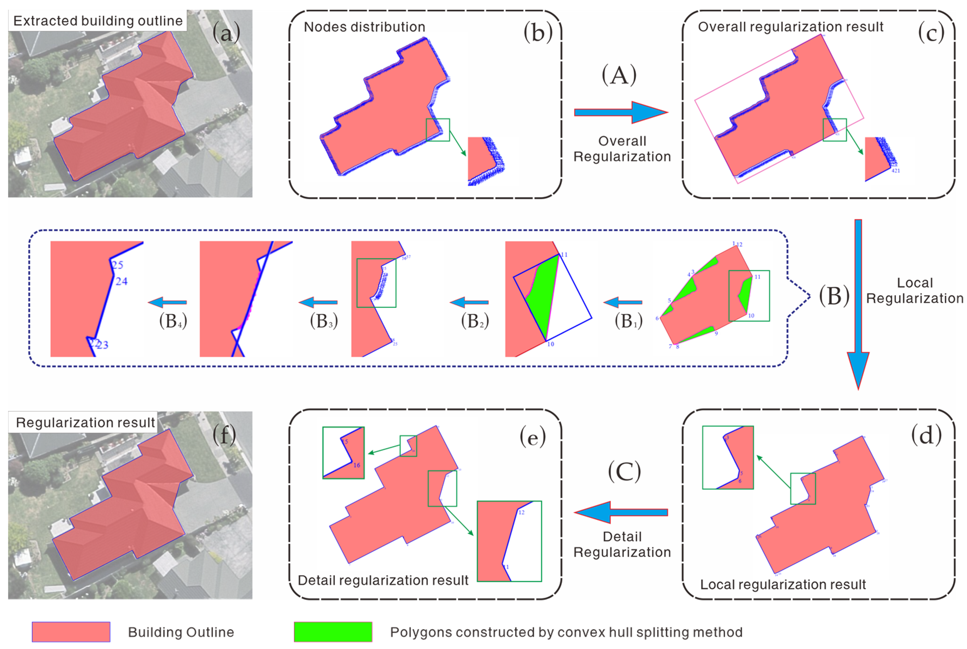
• A new “overall–local–detail” multilevel regularization method was designed for building outlines.

2. Materials and Methods

2.1. Principles and Specific Steps

The principle of the proposed regularization method is as follows: First, based on the overall morphological characteristics of the building outline, the MBR is combined with the Hausdorff distance to perform overall regularization of the outline. This step ensures that the overall morphology and main orientation of the building outline are preserved as effectively as possible before and after regularization. Then, based on its complexity, the building outline is progressively split and locally regularized in a hierarchical manner to preserve the key details of complex outlines. Finally, considering building outline properties, such as parallelism, perpendicularity, normalization, and orthogonality, the building outline is further refined to make it more consistent with the actual characteristics of the building. The specific process consists of three steps (as shown in Figure 1).

Step 1: Overall Regularization (Process A).

First, the MBR of the building outline is calculated. Then, the parts of the original building outline whose Hausdorff distance from the MBR is less than a specified threshold are replaced with corresponding line segments on the MBR. This process yields the overall regularization result, as shown in Figure 1c.

Step 2: Local Regularization (Process B).

Based on the convex hull and node distribution characteristics of the building outline, the non-regularized parts of the outline are divided into multiple line chains and classified into three categories: point-like, line-like, and area-like. Then, each category is regularized separately. Complex line chains are iteratively split and classified for further regularization. As shown in Figure 1, after the splitting and regularization process from B₁ to B₂, locally unregularized parts remain in the building outline. Thus, it is necessary to continue classifying and regularizing the unregularized parts, as shown in the process from B₃ to B₄ in Figure 1. After processing all of the nodes, the local regularization result is obtained, as shown in Figure 1d.

Step 3: Detail Regularization (Process C).

Based on the characteristics of the building outline, acute convex nodes, duplicate nodes, collinear nodes, and missing nodes are processed. Parallel and perpendicular relationships are also strengthened to obtain the detailed regularization result, as shown in Figure 1e.

In Figure 1, a comparison between Figure 1b,e reveals that the initial building outline extracted using deep learning has redundant nodes and jagged edges and lacks clear corner points. After regularization, the number of nodes is significantly reduced, the edges are more regular, and the corner points are clear, highlighting the parallel and orthogonal elements.

2.2. Overall Regularization of Building Outlines Using Hausdorff Distance and MBR

The Hausdorff distance algorithm measures the similarity between two sets of sample points in space by calculating the distance between them [22]. Because vectorized building outlines can be represented as ordered sets of points in space, the Hausdorff distance algorithm can be used to measure the dissimilarity between the outline of a building and its MBR. By setting a threshold, parts of the original building outline with Hausdorff distances smaller than the threshold are superseded using corresponding line segments on the MBR, achieving the partial regularization of the building outline.

2.2.1. Calculation of Hausdorff Distance

Given two point sets P = {P₀, P₁, P₂, P₃, …, P_m} and Q = {Q₀, Q₁, Q₂, Q₃, …, Q_n} in Euclidean space, the distance between these two point sets can be measured by the Hausdorff distance, which is defined as follows:

$$H\left(P,Q\right)=max\left[h\left(P,Q\right),h\left(Q,P\right)\right],$$

(1)

$$\left\{\begin{array}{c}h(P,Q)=\underset{p\in P}{max} \underset{q\in Q}{min}‖p-q‖ \\ h(Q,P)=\underset{q\in Q}{max} \underset{p\in P}{min}‖q-p‖ \end{array}\right.,$$

(2)

where ||p − q|| is the Euclidean distance between points p and q, h(P,Q) is the one-way Hausdorff distance from point set P to point set Q, h(Q,P) is the one-way Hausdorff distance from point set Q to point set P, and H(P,Q) is the two-way Hausdorff distance.

As shown in Figure 2a, if the nodes of two building outlines are represented as two ordered point sets P and Q, the Hausdorff distance method can be used to calculate the Hausdorff distance between any line segment P_iP_i+1 on building outline P and any line segment Q_jQ_j+1 on building outline Q.

The calculation method is illustrated in Figure 2b. Firstly, line segment P_iP_i+1 is equally divided into t segments, and line segment Q_jQ_j+1 is equally divided into s segments. Then, the Euclidean distance between each division point P_ik (k = 0, 1, 2, …, t) on line segment P_iP_i+1 and each division point on line segment Q_jQ_j+1 is calculated to obtain the minimum distance. In Figure 2b, H_i0 and H_ik represent the minimum distances corresponding to points P_i0 and P_ik, respectively. After obtaining the minimum distances for all divided points on building outline P, the maximum value among all the minimum distances is taken as the one-way Hausdorff distance $h(P,Q)$ from line segment P_iP_i+1 to line segment Q_jQ_j+1. Then, $h(Q,P)$ and $H(Q,P)$ can be similarly calculated.

2.2.2. Building Outline Regularization Using the Hausdorff Distance Method and Its Improvement

Wang et al. [15] and Chang et al. [22] applied the Hausdorff distance method to the regularization of building outlines. Their method can be summarized as follows: let P_build and Q_rect denote the line segments on the building outline and MBR, respectively, and set a threshold u. Then, replace line segments P_build on the building outline of Hausdorff distances less than u with the corresponding line segments Q_rect on the MBR, as illustrated in Figure 3. Specifically, if $h\left(P,Q\right)$< u, replace the line segment on the building outline with the corresponding line segment on the MBR. If $h\left(P,Q\right)$ > u, further divide this line segment into multiple segments; then, replace the line segments on the building outline of Hausdorff distances less than u with the corresponding segments on the MBR, while keeping the rest of the segments unchanged.

The definition of u is given by Equation (3):

$$u=\frac{S_{build}}{S_{mrb}}\times \frac{L_{short}}{2}\times \omega ,$$

(3)

where $S_{build}$ is the enclosed area of the building outline; $S_{mrb}$ is the area of the MBR; $L_{short}$ is the length of the shorter side of the MBR; and $\omega$ is a scaling factor, $\mathsf{\delta }\le \omega <1$. If the value of $u$ is set equal to the data resolution value, the minimum value $\mathsf{\delta }$ of the range of $\omega$ can be obtained. After several experiments, it is known that $\mathsf{\delta }$ can be used as the initial value of $\omega$ for regularization. When the regularization results are unsatisfactory, $u$ can be adjusted to an appropriate value by gradually increasing the scaling factor $\omega$.

The accuracy of the Hausdorff distance calculation between two line segments given in Section 2.2.1 depends on the number of segment divisions; using fewer divisions results in lower accuracy, whereas using more divisions increases the computational complexity. In addition, the accuracy of the Hausdorff distance directly impacts the precision of building outline regularization. Because a building outline extracted from remote sensing images consists of line segments connected by straight lines between adjacent nodes, as shown in Figure 2b, the minimum Euclidean distance H_ik from division point P_ik on line segment P_iP_i+1 to the nearest division point Q_jf on line segment Q_jQ_j+1 must either linearly increase or decrease from H_i0 to H_im. Therefore, the Hausdorff distance must necessarily be achieved at one of the endpoints of a line segment. Accordingly, this study proposes an improved algorithm for building outline regularization using the Hausdorff distance and MBR as follows:

1.

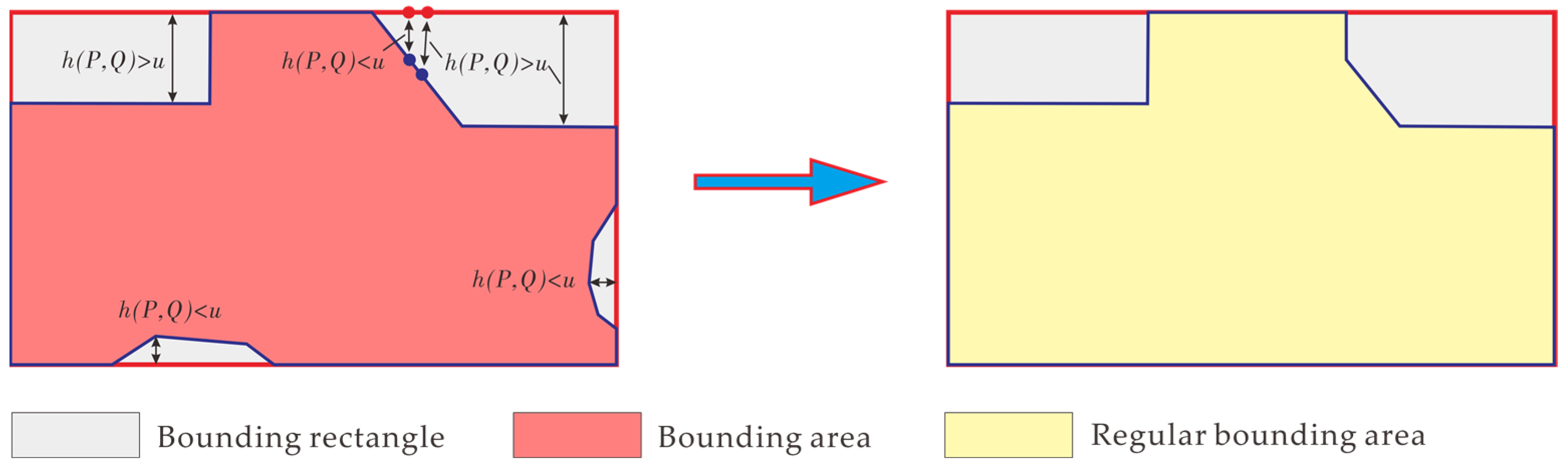
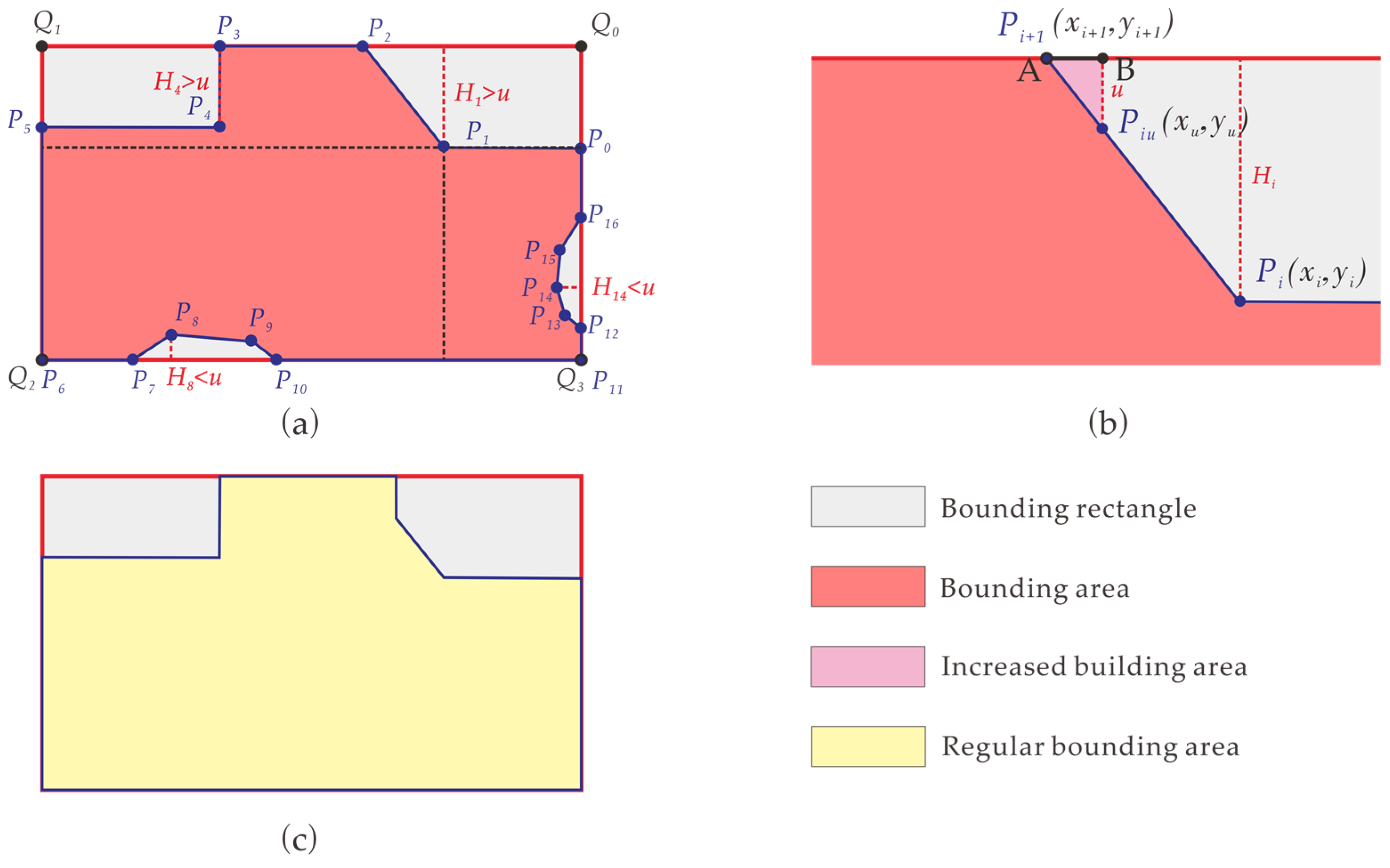
Take the ordered set of nodes from the building outline as the point set P and treat the four corner points of the MBR as the point set Q. Then, in sequence, calculate the perpendicular distance from each point in set P to the line segments formed by adjacent points in set Q. Use the minimum distance among the four distances as the distance H_i from point P_i to the MBR. As shown in Figure 4a, calculate the perpendicular distances from point P₁ to line segments Q₀Q₁, Q₁Q₂, Q₂Q₃, and Q₃Q₀, and then, select the minimum distance H₁ as the distance from point P₁ to the MBR.

2.

For any line segment P_iP_i+1 on the building outline, take the larger of H_i and H_i+1 as $h(P,Q)$.

3.

If $h(P,Q)$ < u, replace the line segment on the building outline with the corresponding orthographically projected line segment on the nearest edge of the MBR. If $h\left(P,Q\right)$ > u, there are two possible cases: either both endpoints of the line segment are farther from the MBR than u, in which case the outline segment remains unchanged, or only one endpoint has a distance greater than u from the MBR. In the latter case, use Equation (4) to calculate point (x_u, y_u) on the line segment where the distance to the MBR equals u, and replace the part of Hausdorff distances less than u with the corresponding segments on the MBR.

$$\left\{\begin{array}{c}{x}_u=x_i+\frac{(x_{i+1}-x_i)\times (u-H_i)}{H_{i+1}-H_i}\\ y_u=y_i+\frac{(y_{i+1}-y_i)\times (u-H_i)}{H_{i+1}-H_i}\end{array}\right.,$$

(4)

where H_i and H_i+1 are the minimum distances from the endpoints P_i and P_i+1 of the line segment, respectively, to an edge of the MBR.

In Figure 4b, where H_i > u and H_i+1 = 0, the coordinates of point P_iu can be calculated. Then, replace the part of the line segment from P_iu to P_i+1 whose Hausdorff distance is smaller than u with the corresponding orthographically projected line segment AB on the nearest edge of the MBR.

4.

After iteratively processing all points on the building outline, the overall regularization result is obtained, as shown in Figure 4c.

The original Hausdorff distance method is highly versatile. In addition to being suitable for measuring the similarity between straight line segments, it can be applied to measure the similarity between curved line segments. In this paper, the calculation process was optimized by considering the linear nature of building outline features extracted from remote sensing images. Figure 5 compares the pre- and post-optimization methods. Figure 5a demonstrates the regularization process using the pre-optimization Hausdorff distance method, which firstly divides line segments P and Q into several smaller segments by equidistant points, computes $h(P,Q)$ for each segment on P, and then replaces line segment AB, for which $h\left(P,Q\right)$ < u, with the corresponding CD on Q. Figure 5b presents the post-optimization Hausdorff distance method, which calculates point F located on line segment P with a perpendicular distance of u from line segment Q and computes the corresponding perpendicular foot H on Q. Then, line segment EF, for which $h(P,Q)$ < u, is replaced with the corresponding line segment GH on Q.

The proposed method reduces the need for segment division and separates the Hausdorff distance. Instead, line segments on P whose Hausdorff distances are less than or equal to the threshold are directly calculated and replaced. We compared the computational efficiency of the Hausdorff distance regularization algorithm before and after the improvement by selecting 300 buildings each from the two resolutions of 0.075 m and 0.5 m data, respectively. We set the parameters t = 5, s = 10, and u = 0.15 for the data with a resolution of 0.075 m and t = 5, s = 10, and u = 1 for the data with a resolution of 0.5 m. The time statistics used are listed in

Table 1. Comparison of computational efficiency before and after improving the Hausdorff distance method.

Data Resolution	Pre-Improvement	Post-Improvement	Efficiency Improvement
0.075 m	1:38′56″	3′26″	96.53%
0.5 m	16′21″	1′05″	93.83%

.

As can be seen from Table 1, the computational efficiency of the improved Hausdorff distance algorithm has been significantly improved. The higher the resolution of the data, the greater the improvement. Moreover, the pre-optimization Hausdorff distance method relies on increasing the number of division points to find points on P that are infinitely close to a perpendicular distance of u from Q, which may introduce errors. By contrast, the proposed method directly calculates points on P that have perpendicular distances equal to u from Q, resulting in higher accuracy. Thus, the proposed Hausdorff distance optimization algorithm specifically tailored for building outline regularization achieves higher computational efficiency and precision than the original method.

2.2.3. MBR Calculation Method and Its Improvement

Most building outlines have rectangular shapes, either in their entirety or locally. Therefore, the MBR method has been widely applied in the regularization of building outlines. There are two common types of MBRs: the minimum area bounding rectangle (MABR) and minimum perimeter bounding rectangle (MPBR). For building outlines with clear orthogonal features or simple structures, little difference exists between these two MBR types. However, for non-orthogonal or complex building outlines, differences may arise.

The algorithms for MABR and MPBR follow a similar approach: both compute the MBRs for the building outline in all directions and select the one with the smallest area or perimeter as the result. In practice, owing to the unique nature of building outlines, calculating the MBRs aligned with the edges of the convex hull before making a comparison is sufficient [23]. The specific steps are as follows:

1.

Employ the Graham scan algorithm [24] to compute the convex hull of the building outline, as shown in Figure 6a,b.

2.

Calculate all MBRs aligned with the edges of the convex hull and record the area and perimeter for each direction, as depicted in Figure 6c.

3.

Select the MBR with the smallest area as the MABR and the one with the shortest perimeter as the MPBR, as illustrated in Figure 6d, where the green rectangle represents the MABR, and the pink rectangle represents the MPBR of the building outline.

Maintaining the area is an important principle to consider during the regularization of building outlines. The regularization process should minimize changes in area. Therefore, in most cases, the MABR is chosen as the reference for regularization, resulting in satisfactory outcomes. However, for building types such as A and B in Figure 7a, situations arise in which the main orientation of the MABR does not align with the primary orientation of the building outline.

Considering that building outlines extracted from high-resolution remote sensing images have many densely distributed nodes, Kwak and Habib [1] proposed an improved MBR algorithm to solve this issue. Firstly, they calculated the MBRs in various directions for the building outline. Then, they computed the number of nodes on the building outline for which the distance to each MBR outline is shorter than the preset threshold. Finally, they selected the MBR with the maximum number of containing nodes as the result, as shown in Figure 7b. Their method performs well for building outlines with uniformly distributed nodes but may introduce significant errors for building outlines C and D, which have uneven node distributions. As illustrated in Figure 7c, building outline C has a high node density near the corners. Often, building outline extraction from remote sensing images can miss details near the corners, making the corner shapes beveled and leading to errors in the calculated results.

As the Hausdorff distance can measure the similarity between two line chains in Euclidean space, it was introduced to effectively address the errors mentioned above. Thus, an MBR algorithm based on Hausdorff distance was proposed to obtain MBRs with higher similarity to the building outline. The specific steps are as follows:

1.

Compute the convex hull of the building outline.

2.

Calculate the MBRs corresponding to each edge of the convex hull.

3.

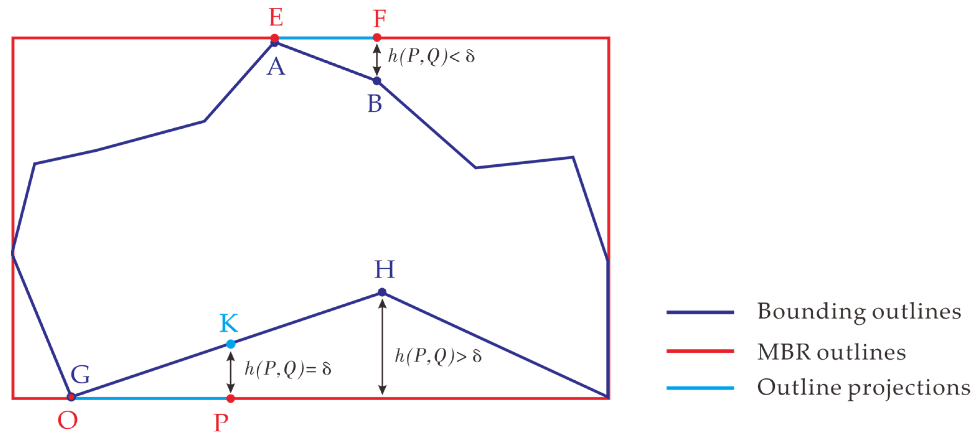
Set a threshold δ (based on extensive experiments, δ can be set to the same value as the data resolution, e.g., 0.5 m for data with resolution of 0.5 m). If the line segment on building outline P to any side of the MBR Q satisfies $h\left(P,Q\right)$< δ, record the length of the projected line segment on Q. As shown in Figure 8, because segment AB satisfies $h\left(P,Q\right)$< δ, the length of its projected line segment EF on Q is recorded. For a line segment satisfying $h\left(P,Q\right)$> δ, if there is a part with $h\left(P,Q\right)$< δ, record the length of the projected segment of that part on Q. As shown in Figure 8, part GK of line segment GH satisfies $h(P,Q)$ < δ, and thus the length of its projected line segment OP on Q is recorded. Then, calculate the ratio p = L_sum/C_rec, where L_sum is the sum of the lengths of projected segments on the current MBR outline, and C_rec is the perimeter of the MBR.

4.

Select the MBR corresponding to the maximum p value as the result based on the Hausdorff distance.

The MBR calculation results based on the Hausdorff distance are presented in Figure 7d. A comparison with the MABR calculation results in Figure 7a shows that the results of the proposed method are generally consistent for most building outlines. Nonetheless, for building types such as A and B, the MABRs obtained using the proposed method align more closely with the overall orientation of the building outline. Figure 7b shows the results of the algorithm based on the MBR with the maximum number of containing nodes. Compared with the results of the proposed method, the results of this algorithm are generally consistent for most building outlines. However, situations with severely offset orientations may occur for building outlines with uneven node distributions, such as building outlines C and D. The superior performance of the proposed method can be attributed to the fact that it simulates manual drawing and uses the Hausdorff distance to measure the similarity between building outlines and MBRs in various directions quantitatively and selects the one with the highest similarity as the result.

We selected 300 buildings from the data with a resolution of 0.075 m and compared our proposed MBR calculation method with the MABR method and the MBR calculation method based on the highest number of collinear nodes. Owing to the lack of manual measurement data for the main direction of buildings and the lack of a unified method for calculating the main direction of buildings, we could only manually observe and judge on a case-by-case basis whether the calculation results are correct. The statistical results of the calculation are shown in

Table 2. Comparison of the accuracy of different MBR calculation methods.

Method	Total Number of Buildings	Number of Correctly Counted	Correct Ratio
MABR	300	263	87.67%
Maximum number of co-linear nodes method	300	286	95.33%
Proposed method	300	300	100%

. It can be seen that the accuracy of our proposed method is 100%, which is higher than the other two methods.

2.3. Local Regularization of Building Outline-Based Convex Hull Grouping

2.3.1. Grouping Unregularized Nodes Using the Convex Hull Method

During the overall regularization stage, only the parts of the building outline with Hausdorff distances less than a set threshold to the MBR are subjected to regularization. To split and classify unregularized parts further, the convex hull of the building outline and node distribution characteristics are considered. The splitting and classification method is described below.

Step 1: For each pair of adjacent nodes T_i and T_i+1 in convex hull point set T of the building outline, identify two points P_m = T_i and P_n = T_i+1 at the same positions in the initial point set P of the building outline. Then, form a node set V = {P_m+i, P_m+i+1, …, P_n-j} based on the continuous and unregularized nodes within the interval from P_m to P_n of point set P.

Step 2: Based on the number of points in set V, as well as the shorter side length l, area s, and length–width ratio r of the MBR formed by V, make an overall judgment of the overall outline characteristics, size, and spatial distribution of the point set, and categorize set V into three types: a point-like node set (Figure 9a), a line-like node set (Figure 9b), and an area-like node set (Figure 9c).

2.3.2. Regularization of Point-like Node Set Using Centroid Coordinate Replacement

The regularization of a point-like node set involves two main steps:

Step 1: Calculate the centroid coordinates of the node set. The centroid coordinates can be solved by forming nonoverlapping triangles using the nodes of the set and computing the centroid (x_i, y_i) and area S_i for each triangle. The centroid coordinates (x_c, y_c) are then computed based on Equation (5):

$$\left\{\begin{array}{c}{x}_c=\frac{\sum S_i{x}_i}{\sum S_i}\\ y_c=\frac{\sum S_i{y}_i}{\sum S_i}\end{array}\right..$$

(5)

Step 2: Replace the points in the point-like node set V_i with a single point at the centroid coordinates (x_c, y_c), without changing its starting and ending points.

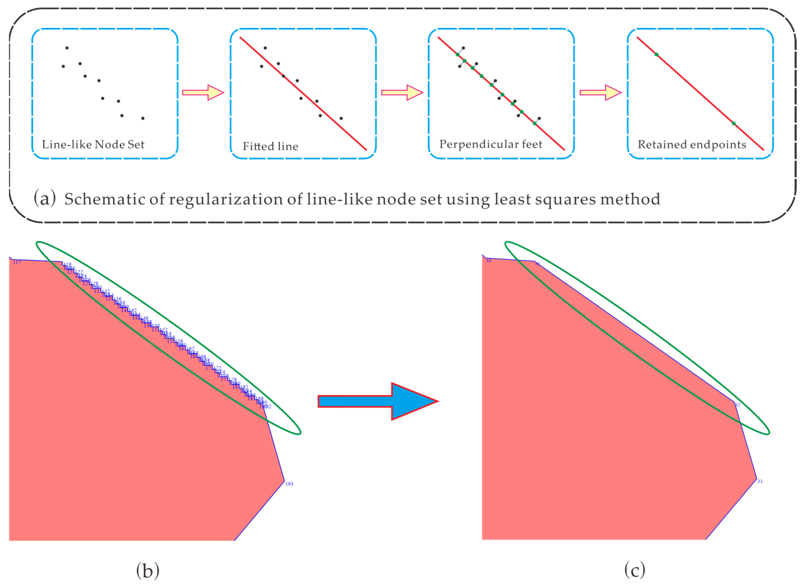
2.3.3. Regularization of Line-like Node Set Using Least Squares Method

The least squares method is an algorithm for fitting n points to minimize the overall error of their distances to a fitted line. It can be used to fit the boundaries of building outlines with noise. The calculation process assumes that the equation of the fitted line for point-like set V_i = {V_i0, V_i1, V_i2, V_i3, …, V_in} is y = kx + b, and it seeks the values of k (Equation (7)) and b (Equation (8)) that minimize the residual sum of squares (RSS) (Equation (6)).

$$RSS=min{\sum }_{i=0}^n{e}_i^2=\underset{a,b}{min}{\sum }_{i=0}^n{[y_i-\left({kx}_i+b\right)]}^2$$

(6)

$$k=\frac{n{\sum }_{i=0}^n{x_{i}y}_i-{\sum }_{i=0}^n{x}_i\times {\sum }_{i=0}^n{y}_i}{n{\sum }_{i=0}^n{x}_i^2-({{\sum }_{i=0}^n{x}_i)}^2}$$

(7)

$$b=\frac{{\sum }_{i=0}^n{y}_i-k{\sum }_{i=0}^n{x}_i}{n}$$

(8)

when $n{\sum }_{i=0}^n{x}_i^2-{({\sum }_{i=0}^n{x}_i)}^2=0$, the slope k of the straight line becomes infinitely large. In this case, the equation of the line is $x=\frac{{\sum }_{i=0}^n{x}_i}{n}$.

Then, the perpendicular feet of all points in the set V_i onto the fitted line are solved, and the two points with the highest and lowest y values (or, if the y values are equal, those with the highest and lowest x values) are determined. The two points are grouped into a new set to replace point set V_i. The specific process is illustrated in Figure 10.

2.3.4. Regularization of Area-like Set Using the Hausdorff Distance Method

For the building outline P extracted from Figure 11a, the results obtained after applying the regularization method given in Section 2.2 are shown in Figure 11b. The convex hull method is used to group the unregularized nodes, resulting in four area-like sets V_i, V_j, V_k, and V_t, where V_i = {P₁, P₂, P₃, …, P₂₂₈}, V_j = {P₂₂₉, P₂₃₀, P₂₃₁, …, P₃₃₂}, V_k = {P₃₃₃, P₃₃₄, P₃₃₅, …, P₅₇₃}, and V_t = {P₅₇₄, P₅₇₅, P₅₇₆, …, P₆₇₅}.

The regularization process for the area-like set is as follows:

1.

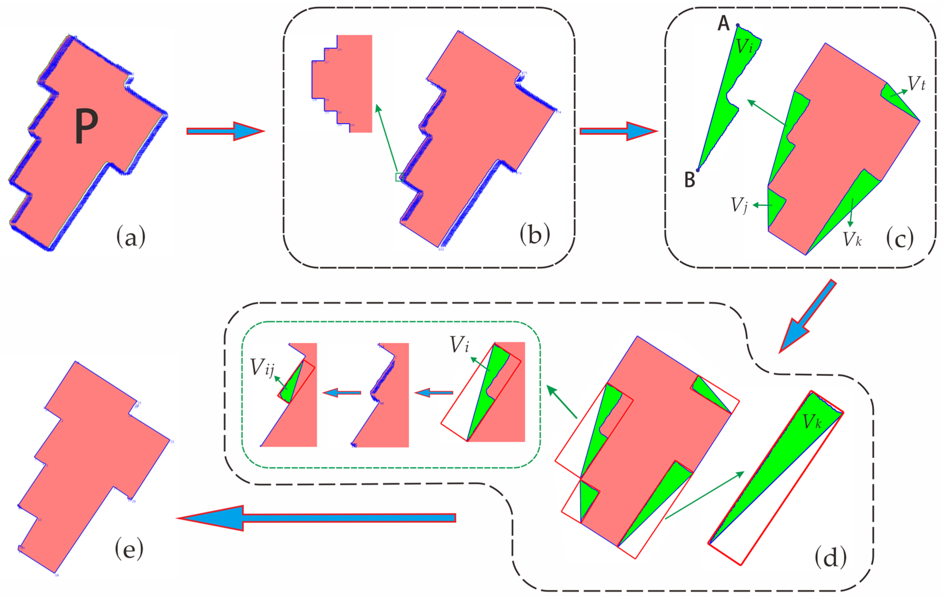
Connect the starting and ending nodes of the area-like set to form a closed surface. Regularize it using the method described in Section 2.2. The difference here is that, when calculating the MBR and using the Hausdorff distance method for regularization, only the line segments composed of adjacent nodes that belong to the building outline are calculated and processed. Line segments that overlap with the convex hull outline and do not belong to the building outline are not considered. As shown in Figure 11c, during the regularization of V_i, segment AB is not part of the building outline. Thus, including it in calculations may affect the regularization results.

2.

Continue to calculate the convex hull for area-like set V and construct unregularized point sets by category. Figure 11d shows the regularization of area-like sets V_i, V_j, V_k, and V_t, as well as the continued use of the convex hull method to split and classify the unregularized portions of V_i.

3.

Iteratively execute the above steps. Once all nodes have been processed, local regularization results are obtained.

2.4. Detailed Regularization and Enhancement of Parallel and Perpendicular Relationships

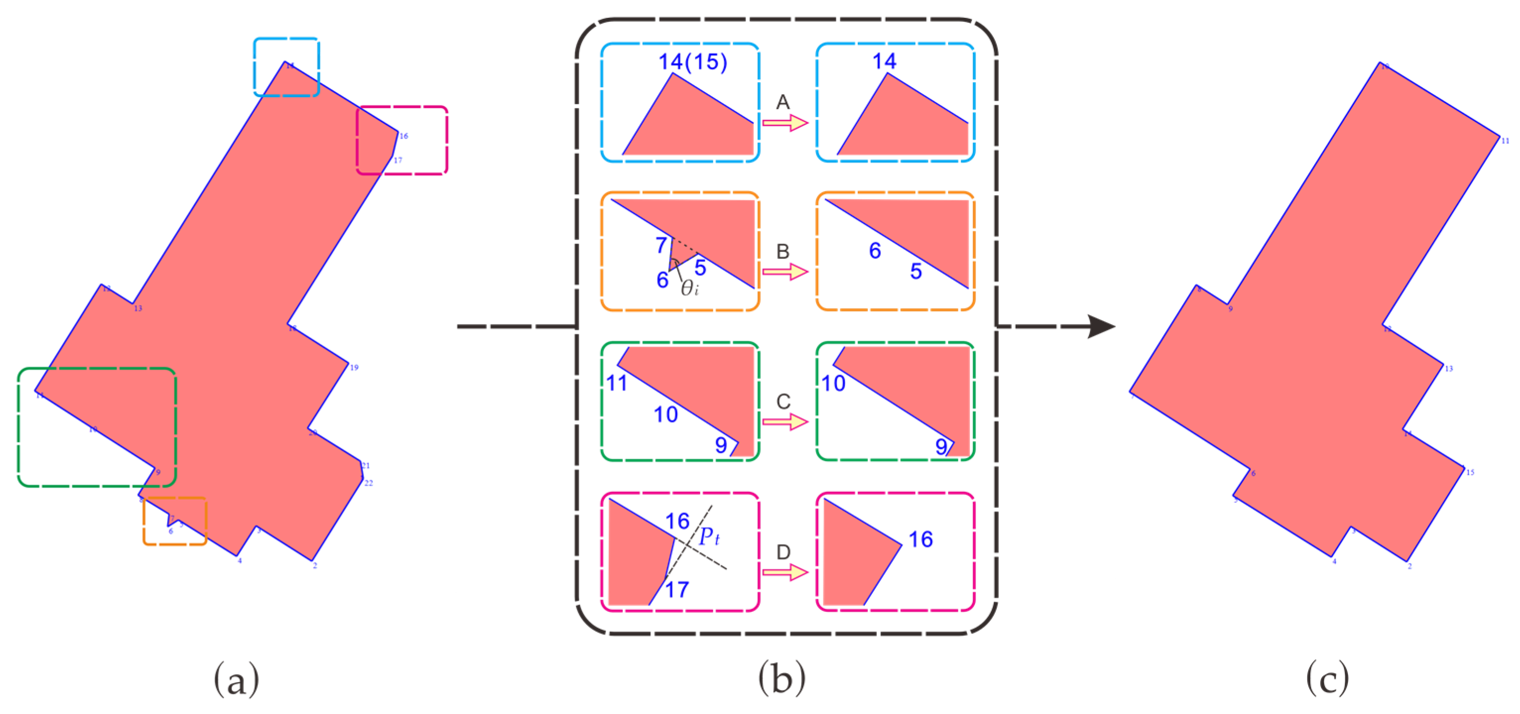
2.4.1. Detailed Regularization

Detailed regularization primarily eliminates repetitive nodes, collinear nodes, and acute concave nodes on building outlines and completes missing corner nodes.

Elimination of Repetitive Nodes: When the positions of two adjacent points (P_i, P_i+1) in the building outline nodes are equal or approximately equal, only one of them is retained. Duplicate nodes can be determined by setting a distance threshold d. If the Euclidean distance d_i(i+1) (P_i, P_i+1) between two adjacent points is shorter than d, these points are considered repetitive nodes. Typically, d can be set to 0.1 m. For example, in Figure 12b, nodes 14 and 15 during Process A are considered repetitive nodes, as the Euclidean distance between them is less than d, and node 15 is deleted.

Elimination of Acute Concave Nodes: When a point P_i on the building outline deviates from the main outline, it forms a sharp triangle with the preceding and succeeding nodes P_i−1 and P_i+1. In this case, point P_i becomes an acute concave node and should be deleted. Whether a node is an acute concave node can be judged based on angle threshold α and area threshold S. If angle α_i of the acute corner or area S_i of the jagged triangle is less than the respective threshold (α or S), point P_i is considered an acute concave node. Typically, α can be set to 5°, and the value of S depends on the data resolution, with higher resolutions requiring smaller S values. For instance, in Figure 12b, during Process B, node 6 and the triangle formed by it with the preceding and succeeding nodes 5 and 7 have an area smaller than S; thus, node 6 is deleted.

Elimination of Collinear Nodes: When the segment between node P_i on the building outline and its preceding node P_i−1 is parallel or approximately parallel to the segment between node P_i and its succeeding node P_i+1, the middle node P_i should be eliminated. Whether a node is collinear is determined based on angle threshold β. If |180° − β_i| < β, where β_i is the angle of the broken lines formed by the three adjacent nodes with P_i as the vertex, then P_i is considered a collinear node. Typically, β can be set to 1°. For example, in Figure 12b, during Process C, nodes 9, 10, and 11 form angle β_i at vertex 10, which satisfies |180° − β_i| < β; thus, node 10 is deleted.

Completion of Corner Nodes: Building outlines extracted from remote sensing images often have sloping corners because not every corner is successfully extracted. These corners must be completed by extending segments P_i−1P_i and P_i+2P_i+1 that precede and succeed segment P_iP_i+1 until they intersect at point P_t. Then, area S_i and the smallest internal angle α_i of triangle P_tP_iP_i+1 are calculated. Thresholds α and S are set similarly to those in the processing method for acute concave nodes. If S_i < S or α_i < α, node P_i is replaced with P_t, and node P_i+1 is deleted. In Figure 12b, during Process D, the extended lines of segments 15–16 and 18–17 intersect at point P_t, and the triangle formed by P_t and nodes 16 and 17 has an area smaller than S. Therefore, node 16 is replaced with P_t, and node 17 is deleted.

2.4.2. Enhancement of Parallel and Perpendicular Relationships Based on the Main Direction of the Building Outline

After the “overall–local–detail” stepwise regularization process, the building outline becomes more regular. However, building outlines are mostly composed of polygons with the adjacent edges being perpendicular and opposite edges being parallel. Therefore, the parallel and perpendicular relationships in the building outline must be enhanced to make them more realistic. In this study, we took the long side of the MBR of the building outline as the main direction and performed parallel and perpendicular enhancements. The specific steps are as follows:

1.

Calculate the MBR of the building outline and take one of its long sides as vector a.

2.

Calculate the angles θ between vectors b (consists of two neighboring nodes) and a in a counterclockwise direction, as described by Equation (9):

$$\theta =180\times \frac{\mathit{arccos}\left(\frac{\overrightarrow{\mathit{a}}\times \overrightarrow{\mathit{b}}}{\left|\overrightarrow{\mathit{a}}\right|\times \left|\overrightarrow{\mathit{b}}\right|}\right)}{\pi } (0\le \theta \le 180).$$

(9)

3.

Set a threshold γ to 15°. If $\theta \in \left(90-\gamma ,90+\gamma \right)$, then the line segment is approximately perpendicular to the main direction, and the method shown in Figure 13a is applied. A line is drawn through the midpoint P_m of line segment P_iP_i+1, perpendicular to the main direction. This line intersects the extensions of the two adjacent line segments at points P_i′ and P_i+1′. Replace P_i with P_i′ and P_i+1 with P_i+1′. If $\theta \in \left(180-\gamma ,180\right)$ or $\theta \in \left(0,\gamma \right)$, then the line segment is parallel to the main direction, and the method shown in Figure 13b is applied. After that, a line is drawn through the midpoint P_n of line segment P_jP_j+1, parallel to the main direction. This line intersects the extensions of the adjacent two line segments at points P_j′ and P_j+1′. Replace P_j with P_j′ and P_j+1 with P_j+1′. If the line segment is not parallel or perpendicular to the main direction, no further action is taken, as shown in Figure 13c.

3. Experimental Design

3.1. Descriptions of the Datasets

We evaluated the proposed method using the open-source WHU Building Dataset [25], which covers a 450 km² area in Christchurch, New Zealand. This dataset includes approximately 220,000 independent buildings of various types and structures. Owing to its wide coverage, high-quality imagery, large dataset size, and diverse building types, this dataset has become very popular for research on building extraction and regularization methods. A region within the coordinate ranges of 43°32′48″ to 43°33′17″ South latitude and 172°41′14″ to 172°41′58″ East longitude was randomly selected as Image #1. This image, shown in Figure 14, has an original spatial resolution of 0.075 m and contains 932 buildings.

To assess the effectiveness of the proposed method comprehensively, Image #1 was down-sampled to a spatial resolution of 0.5 m, creating Image #2. Then, the deep learning technique proposed by Qiu et al. [26] was applied to both Images #1 and #2 to extract building outlines at two different levels of accuracy. These extracted building outlines served as the experimental data for the proposed regularization method. Figure 15 presents examples of the original 0.075 m resolution remote sensing image, manually labeled ground truth, and building outlines extracted from both resolutions using the deep learning technique.

3.2. Experimental Settings

The proposed algorithm was developed using the C++20 programming language on the GenerMap V3.0 secondary development software platform, which was self-developed based on Visual Studio 2019. To better evaluate the performance of our proposed method, we selected three comparison methods: Wei et al. [19] proposed a method for extracting building outlines from remotely sensed images and a regularization algorithm consisting of coarse and fine adjustments for extracting building outlines from remotely sensed images, and we use their proposed regularization method as Method A. Bayer [27] proposed a more classical iterative building outline simplification algorithm, which realizes the regularization of the building outline data extracted from remote sensing images by setting the threshold compatible with the resolution of the data, and we use it as Method B; Feng et al. [28] proposed a regularization method with patching performance to extract building outlines from remotely sensed images, which we refer to as Method C. We evaluated the accuracy and superiority of our proposed method by regularizing the data at a resolution of 0.075 m using three comparison methods and the method in this paper. In addition, the regularization results of various methods for images with both 0.075 m and 0.5 m resolutions were compared to assess the applicability of the proposed method.

3.3. Evaluation Metrics

The regularization results were evaluated from both quantitative and qualitative perspectives. Following references [5,19,29,30], common evaluation metrics, including precision P, recall R, intersection over union (IOU), and F1 score, were adopted to assess the extraction results quantitatively. Larger percentages indicate better algorithm performance. Specifically, F1 is the harmonic mean of precision and recall. The calculation methods for each evaluation metric are as follows:

$$\mathrm{P}=\frac{{\mathrm{S}}_{\mathrm{r}\mathrm{e}\mathrm{s}\mathrm{u}\mathrm{l}\mathrm{t}\cap \mathrm{r}\mathrm{e}\mathrm{f}\mathrm{e}\mathrm{r}\mathrm{e}\mathrm{n}\mathrm{c}\mathrm{e}}}{{\mathrm{S}}_{\mathrm{r}\mathrm{e}\mathrm{s}\mathrm{u}\mathrm{l}\mathrm{t}}},$$

(10)

$$\mathrm{R}=\frac{{\mathrm{S}}_{\mathrm{r}\mathrm{e}\mathrm{s}\mathrm{u}\mathrm{l}\mathrm{t}\cap \mathrm{r}\mathrm{e}\mathrm{f}\mathrm{e}\mathrm{r}\mathrm{e}\mathrm{n}\mathrm{c}\mathrm{e}}}{{\mathrm{S}}_{\mathrm{r}\mathrm{e}\mathrm{f}\mathrm{e}\mathrm{r}\mathrm{e}\mathrm{n}\mathrm{c}\mathrm{e}}},$$

(11)

$$\mathrm{I}\mathrm{O}\mathrm{U}=\frac{{\mathrm{S}}_{\mathrm{r}\mathrm{e}\mathrm{s}\mathrm{u}\mathrm{l}\mathrm{t}\cap \mathrm{r}\mathrm{e}\mathrm{f}\mathrm{e}\mathrm{r}\mathrm{e}\mathrm{n}\mathrm{c}\mathrm{e}}}{{\mathrm{S}}_{\mathrm{r}\mathrm{e}\mathrm{s}\mathrm{u}\mathrm{l}\mathrm{t}\cup \mathrm{r}\mathrm{e}\mathrm{f}\mathrm{e}\mathrm{r}\mathrm{e}\mathrm{n}\mathrm{c}\mathrm{e}}},$$

(12)

$$\mathrm{F}1=\frac{2\mathrm{P}\mathrm{R}}{\mathrm{P}+\mathrm{R}},$$

(13)

where S_result is the area of the algorithm regularization result; S_reference is the building area of the reference data; and S_{result∩reference} and S_{result∪reference} are the areas of the intersection and union, respectively, between the regularization result of the algorithm and the reference data. Regarding S_reference, to evaluate the regularization effect comprehensively, the reference data in Experiment 4.1 were the manually labeled ground truth data, whereas those in Experiment 4.2 were the extracted building outline data.

4. Results and Analysis

4.1. Experimental Analysis

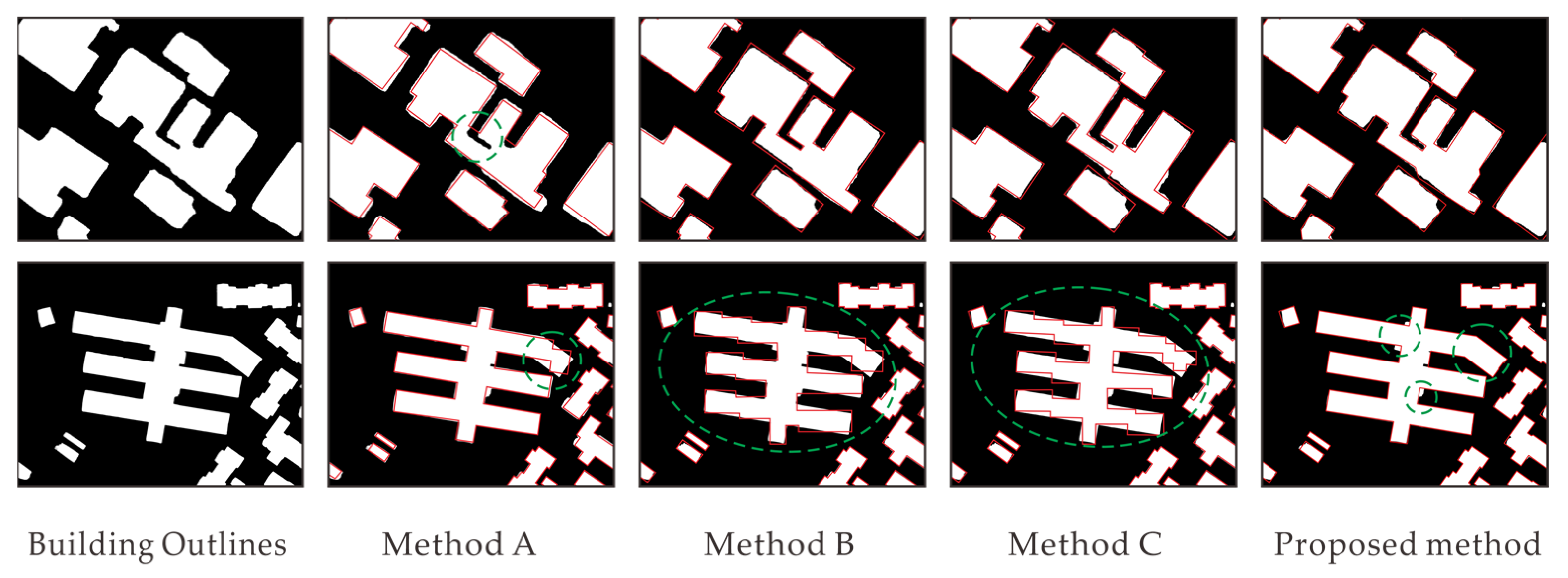
4.1.1. Qualitative Evaluation

Figure 16 presents examples of the regularization results of the four methods for extracting building outlines from the images with 0.075 m resolution, along with the manually labeled ground truths. The top two rows display regularization results for relatively regular building outlines, whereas the bottom three rows show results for more complex building outlines. Comparing the building outlines before and after simplification, all methods clearly achieve satisfactory results in the regularization of relatively regular building outlines, as shown in Figure 16a,b. However, for more complex building outlines, Methods A, B, and C exhibit certain shortcomings, as illustrated in Figure 16c–e. These shortcomings can be categorized into two types: some parts of the complex outline are eliminated through regularization, and some parts that do not align with the main direction of the building outline are excessively regularized.

To visualize and assess the regularization performance of each method better, the regularization results from different methods were overlaid with the manually labeled ground truth, as shown in Figure 17.

Method A divides the building outline regularization process into two steps. The first step is to remove noise points, redundant nodes, and small outline segments. When dealing with densely populated complex outlines, this step may lead to the loss of some outline details. The second step employs the long edge weighting method to determine the main direction and adjusts the line segments composing the outline accordingly. Because only one main direction is used for control, there may be instances where outlines inconsistent with the main direction of the building are over-regularized as shown in Figure 17a. Method B initially rotates the building outline to align the edges of its MBR with the coordinate axes. Then, it divides the building outline into four parts using the four nodes closest to the four vertices of the MBR on the building outline. Each part is iteratively split using the regression line method, and the resulting regression lines satisfying certain conditions are intersected and recombined to obtain the regularization results. This method utilizes the MABR. When a deviation exists between the long edge of the MBR and the main direction, the overall orientation of the regularized outline may deviate from the true outline, as shown by the yellow dashed line inside the building outline in Figure 17b. Moreover, Method B uses a vertical regression processing strategy that maximizes the orthogonality of the building outline. However, it may produce locally inaccurate results for non-rectangular building outlines, as indicated by the blue dashed line inside the building outline in Figure 17b. Method C iteratively employs the MBR to segment and hierarchically organize the building outline, mapping the outlines of each hierarchy to their corresponding MBR to eliminate jagged nodes and regularize the shape of the building. This method performs well for building outlines with clear rectangular features but produces locally inaccurate results for complex building outlines and non-rectangular combinations of building outlines, as shown in Figure 17c. The proposed method is based on the concept of manual sketching when regularizing building outlines. It uses the Hausdorff distance-based MBR to control changes in direction and shape, locally splits and classifies building outlines, and enhances parallel, perpendicular, and orthogonal characteristics. Consequently, the proposed method achieves regularization results that are closer to the manually labeled ground truth than those of the contrasted methods, as shown in Figure 17d.

4.1.2. Quantitative Evaluation

Because the results extracted from the images with 0.075 m resolution exhibit high accuracy and visually resemble the actual building outlines, the manually labeled ground truth was taken as the reference for evaluation. This evaluation reflects the performance of different algorithms in repairing jagged outline data. The statistical evaluation metrics for various methods are summarized in

Table 3. Comparison of regularization results from different methods.

Method	P (%)	R (%)	IOU (%)	F1 (%)
A	91.62	96.74	88.88	94.11
B	94.96	96.45	91.75	95.70
C	93.42	88.85	83.62	91.08
Proposed method	95.97	98.41	94.50	97.17

P: precision; R: recall; IOU: intersection over union; F1:F1 score.

.

As shown in Table 3, Method A has a relatively low P value, indicating that more building areas are classified as nonbuilding areas. This is because during the removal of noise points, redundant nodes, and small line segments, some nodes belonging to building outlines may be mistakenly removed, resulting in the loss of some outline details, which also explains the slightly lower IOU and F1 score values of this method. Method B achieves balanced scores in all evaluation metrics because it employs an iterative approach from overall to local, limiting outline deformation within a certain range. Method C has a relatively low R value, indicating that more nonbuilding areas are classified as building areas. This is because the iterative use of the MBR for splitting and fitting building outlines is likely to classify some nonbuilding areas as buildings, which also leads to the relatively low IOU and F1 score of Method C. The proposed method achieves the highest P and R values of 95.97% and 98.41%, respectively, among the considered methods. This indicates that the proposed method can better complement missed building outline parts during regularization and remove erroneously extracted portions than the other methods. Moreover, the proposed method has the highest IOU (94.50%), signifying that the regularization results of this method have a higher overlap ratio with the manually labeled ground truth than those of any other contrasted method. Furthermore, the proposed method achieves the highest F1 score (97.17%), further demonstrating its superiority and general applicability.

The main reasons that the regularization results of the proposed method are higher than those of the other methods in each index are as follows. First, in the overall regularization phase, the proposed method uses an improved MBR, which is more accurate than the traditionally used MABR. Moreover, in the local regularization phase, the proposed method splits individual building outlines into various types and processes them separately, enhancing the regularization accuracy for non-orthogonal building outlines. Next, in the detailed regularization phase, the proposed method incorporates building orientation and reinforces parallel, perpendicular, and orthogonal characteristics to address acute convex nodes, inaccurate corners, and non-straight segments, mimicking the process of manual sketching while ensuring that our regularization results approximate the manually labeled ground truth.

Besides the accuracy of regularization results, the high efficiency of the regularization method is also valuable in practical applications. The proposed outline optimization method is primarily divided into three stages. The first stage, overall regularization, consists of three steps: (1) MBR calculation with a time complexity of O(n²), (2) regularization based on the Hausdorff distance method with a time complexity of O(n), and (3) removal of redundant points with a time complexity of O(n). Therefore, the time complexity of the first stage is O(n²). The second stage, local regularization, also includes three steps: (1) outline splitting, and classification based on convex hull with a time complexity of O(n²), (2) classification regularization with a time complexity of O(n²), and (3) removal of redundant points with a time complexity of O(n). Thus, the time complexity of the second stage is O(n²). The third stage, detailed regularization and parallel-perpendicular enhancement, involves two steps: (1) detailed regularization with a time complexity of O(n) and (2) parallel–perpendicular relationship enhancement with a time complexity of O(n). Therefore, the time complexity of the third stage is O(n). Thus, the overall time complexity of the proposed method is O(n²).

Table 4. Time complexity of the different methods.

Method	Time Complexity
	First Step	Second Step	Third Step	Sum
A	O(n2)	O(n2)	--	O(n2)
B	O(n2)	O(n2)	O(n)	O(n2)
C	O(n2)	O(n2)	…	O(n2)
Proposed method	O(n2)	O(n2)	O(n)	O(n2)

lists the time complexities of different methods. The time complexities of the four methods are similar; thus, the proposed method achieves better results with a similar time complexity.

4.2. Applicability of Analysis for Data of Different Resolutions

Figure 18 illustrates examples of regularization results for building outlines extracted from images with two different resolutions: 0.075 m and 0.5 m. As shown, for the data with 0.075 m resolution, except for a few complex-shaped buildings, the regularization results from various methods align well with the extracted building outlines, indicating a high level of regularization. However, for the data with 0.5 m resolution, the regularization effects of all methods are reduced to varying degrees. This reduction is primarily characterized by varying degrees of deviation in the main direction of the outlines and a decrease in the overlap ratio between the regularization results and the extracted building outlines.

Comparing the shapes of the outlines for the two different data resolutions in Figure 18 shows that the image resolution has a significant impact on the accuracy of building outline extraction. To prevent the errors introduced during the extraction process from affecting the evaluation of regularization effects, the extracted building outlines were taken as reference data for evaluation.

Table 5. Comparison of regularization results for different methods with two data resolutions.

Data Resolution	Method	P (%)	R(%)	IOU (%)	F1(%)
0.075 m	A	92.43	94.31	87.55	93.36
	B	98.06	97.61	95.76	97.83
	C	96.71	90.16	87.47	93.32
	Proposed method	98.27	98.43	96.75	98.35
0.5 m	A	88.07	94.62	83.87	91.23
	B	94.41	91.58	86.87	92.97
	C	91.28	94.28	86.49	92.76
	Proposed method	92.57	94.82	88.11	93.68

P: precision; R: recall; IOU: intersection over union; F1:F1 score.

displays the regularization metrics for different methods applied to the data of two different resolutions. For both data resolutions, the proposed method achieves the highest IOU and F1 scores, indicating that it more effectively preserves the shape of building outlines during regularization and achieves greater generality. However, as the data resolution decreases, all methods exhibit decreases in the evaluation metrics. The decreases in P and R are attributable to outline deformations and directional deviations, whereas the decline of F1 suggests the weakening generality of these methods. Notably, the IOU decreases more significantly than the other two metrics, suggesting a substantial reduction in the intersection area between the building outlines before and after regularization as the resolution decreases. This is because lower-resolution data lead to more jagged outlines, resulting in greater changes in shape, area, and position during regularization. Furthermore, when applied to the data with 0.075 m resolution, the proposed method outperforms the other methods across all metrics. When applied to the data with 0.5 m resolution, the proposed method continues to outperform other methods in three metrics, but its superiority is less pronounced.

In summary, the proposed method performs well in regularizing building outline data extracted from images with different resolutions. Higher resolutions lead to smaller shape variations during regularization, resulting in more regularized outlines. As the resolution of image data grows, the advantages of the proposed method become more pronounced.

4.3. Analyzing Applicability to Complex Types of Building Outlines

To more comprehensively analyze the applicability and superiority of our proposed method, we selected the regularization results of different types of complex buildings throughout the study area and demonstrated them in comparison with other methods, as shown in Figure 19. It can be seen that for complex types of building outlines, Method A tends to delete the feature points in denser node regions by judging them as interference points, resulting in the loss of part of the outlines—and at the same time—owing to the regularization with respect to only one principal direction, which leads to a large error in regularizing part of the outlines; Method B relies too much on the computational accuracy of MABR, and when the MABR direction is shifted, the building orientation of the regularization result is shifted, and some of the outline details are lost. Method C is good for regularizing the outlines of complex buildings that consist of multiple rectangles with a consistent orientation. However, for complex buildings consisting of multiple rectangles with inconsistent orientation or multiple different shapes, some details of the building will be lost after regularization. Our proposed method uses the processing idea of “whole-local-detail”. As a whole, we use the improved MBR method for direction control, which maintains the direction better than the other three methods; locally, we take the original building outline to be split into several for separate processing, which ensures the accuracy of each part; in detail, we simulate the idea of manual outlining and carry out the repair processing, which effectively removes the unreasonable details. Through comparative analysis, we know that our proposed method effectively improves the problems of other methods, such as insufficiently good overall or local orientation maintenance, poor outline detailing and partial outline loss. For the regularization of complex types of building outlines, our proposed method is more applicable.

4.4. Overall Discussion of the Algorithms and Future Work

The proposed method integrates various techniques, including surface fitting based on an improved Hausdorff distance method and an improved MBR method, line fitting based on the least squares method, and point fitting based on centroid coordinate substitution. The excellent experimental results of the proposed method are because of the improvements of the algorithm. First, a multilevel regularization framework was established, involving three steps: overall regularization, local regularization, and detailed regularization. This framework ensures that building outlines are processed at different levels from the overall to local scales. Second, problems encountered by the commonly used MBR method, including direction deviation and poor fitting to building outlines, were mitigated by improving the MBR method. Consequently, the proposed method can better maintain the consistency of the main direction and overall shape of building outlines during regularization, fundamentally reducing the severity of directional deviations. Third, the Hausdorff distance regularization algorithm was optimized, significantly improving the efficiency and accuracy of regularization. Finally, the process of manual sketching was used as a reference to perform detailed regularization adjustments, making the regularization results closer to the real outlines.

Our proposed method uses building outlines extracted through deep learning techniques as experimental data. The main reason is that the method of extracting building outlines from high-resolution remote sensing images using deep learning techniques is very mature through the research of many scientists, and the extraction results are more accurate and robust. and have better generalization ability compared to traditional extraction methods. Whereas feature extraction in traditional methods mainly relies on the work design of the extractor, which requires specialized knowledge and a complex process of parameter adjustment, the algorithms are application-specific, and the generalization ability and robustness are not as good as in deep learning methods. In the future, with the gradual improvement of the resolution of deep remote sensing images, the advantages of deep learning algorithms will become increasingly obvious, and the application prospects of our proposed method will become broader.

The proposed method is primarily applicable to the regularization of building outlines composed of straight segments. Its applicability in complex building outlines containing curved segments was also tested. Figure 20 shows the regularization results of the proposed method for building outlines with various shapes. As shown, for building outlines composed of straight segments, the proposed method can correct the missing parts of the extracted outlines (Figure 20a) and remove erroneously extracted parts (Figure 20b), making the regularization results closer to the actual building outlines. However, for building outlines that include curved segments, the proposed method outputs polygonal outlines (Figure 20c), indicating that further research is needed to improve regularization in such cases, which will be a focus of future work.

5. Conclusions

Using deep learning and machine learning methods, building patches can be quickly extracted from high-resolution remote sensing images. However, because of the interference of external factors and the errors of the algorithms themselves, the extracted patches have problems such as extraction omissions and extraction errors. After vectorization, these building outlines have low regularization, unclear inflection points, and high data redundancy, which are not suitable for direct use and need regularization. However, there are relatively few studies on regularization methods for building outlines extracted from remote sensing images, and most of the results are unsatisfactory. To improve the application performance of the data and expand the application scenarios, this paper proposes a multi-stage regularization method for the initial building outlines extracted from remote sensing images. Specifically, the proposed method is divided into three steps: overall, local, and detailed regularization. Firstly, an improved Hausdorff distance method was combined with an improved MBR to perform overall building outline regularization. Then, the unregularized parts of the building outline were split into three categories: point-like, line-like, and area-like, based on the convex hull and node distribution of the building outline, and each category was regularized separately. Finally, detailed regularization adjustments and corner orthogonalization were performed based on the characteristics of the building outline to make the regularization results closer to the true outline. Through a large number of experimental verifications, our proposed method can make the data volume of the initial building outline extracted from high-resolution remote sensing images greatly compressed, the degree of regularization greatly improved, and the expression accuracy greatly increased. This can effectively improve the performance and application range of using remote sensing images to extract the building outline. Our proposed method is not only applicable to the building outline with obvious rectangular features but also achieves a better effect on the regularization of the building outline with non-rectangular features. However, for building outlines that contain curved segments, further improvements are needed.

References

1. Kwak, E.; Habib, A. Automatic representation and reconstruction of DBM from LiDAR data using recursive minimum bounding rectangle. ISPRS J. Photogram. Remote Sens. 2013, 93, 171–191. [Google Scholar] [CrossRef]
2. Yan, L.; Li, Y.; Xie, H. Urban building mesh polygonization based on 1-ring patch and topology optimization. Remote Sens. 2021, 13, 4777. [Google Scholar] [CrossRef]
3. Hu, R.; Huang, X.; Huang, Y. An enhanced morphological building index for building extraction from high-resolution images. Acta Geod. Cartogr. Sin. 2014, 43, 514–520. [Google Scholar] [CrossRef]
4. Gao, X.; Wang, M.; Yang, Y.; Li, G. Building extraction from RGB VHR images using shifted shadow algorithm. IEEE Access 2018, 6, 22034–22045. [Google Scholar] [CrossRef]
5. Wang, Y.; Zeng, X.; Liao, X.; Zhuang, D. B-FGC-Net: A building extraction network from high resolution remote sensing imagery. Remote Sens. 2022, 14, 269. [Google Scholar] [CrossRef]
6. Chang, J.; Gao, X.; Yang, Y.; Wang, N. Object-oriented building contour optimization methodology for image classification results via generalized gradient vector flow snake model. Remote Sens. 2021, 13, 2406. [Google Scholar] [CrossRef]
7. Gao, X.; Zheng, X.; Shen, D.; Yang, Y.; Zhang, J. Automatic building extraction based on shadow analysis from high resolution images in suburb areas. Geomat. Inf. Sci. Wuhan Univ. 2017, 42, 1350–1357. [Google Scholar] [CrossRef]
8. Wang, W.X.; Du, J.; Li, X.M.; Hu, H.; Xu, W.; Guo, H.; Ding, Y. A grid filling based rectangular building outlines regularization method. Geomat. Inf. Sci. Wuhan Univ. 2018, 43, 318–324. [Google Scholar] [CrossRef]
9. Ding, Y.; Feng, F.; Li, J.; Hu, Y.; Cui, W. Right-angle buildings extraction from high-resolution aerial image based on multi-stars constraint segmentation and regularization. Acta Geod. Cartogr. Sin. 2018, 47, 1630–1639. [Google Scholar] [CrossRef]
10. Zhou, S.; Sun, J.; Fan, L.; Xiang, J.; Chen, C. Extraction of building contour from high resolution images. Remote Sens. Land Resour. 2015, 27, 52–58. [Google Scholar] [CrossRef]
11. Zhao, K.; Kang, J.; Jung, J.; Sohn, G. Building extraction from satellite images using Mask R-CNN with building boundary regularization. In Proceedings of the 2018 IEEE/CVF Conference on Computer Vision and Pattern Recognition Workshops, Salt Lake City, UT, USA, 18–22 June 2018; pp. 247–251. [Google Scholar] [CrossRef]
12. Douglas, D.H.; Peucker, T.K. Algorithms for the reduction of the number of points required to represent a digitized line or its caricature. Cartogr. Int. J. Geogr. Inf. Geovis. 1973, 10, 112–122. [Google Scholar] [CrossRef]
13. Chang, J.X.; Gao, X.J.; Yang, Y.W.; Wang, S. Building contour optimization method integrating multitemporal and high-resolution images. Bull. Survey. Mapp. 2020, 7, 112–115. [Google Scholar] [CrossRef]
14. Xiang, H.; Jianhua, W.; Ning, W.; Haowen, T. A building contour optimization method for multi-source data. Acta Opt. Sin. 2023, 12, 330–342. [Google Scholar]
15. Wang, S.X.; Yang, Y.W.; Chang, J.X.; Gao, X.J. Optimization of building contours by classifying high-resolution images. Laser Optoelectron. Prog. 2020, 57, 329–338. [Google Scholar] [CrossRef]
16. Shen, W.; Li, J.; Chen, Y.H.; Deng, L.; Peng, G.X. Algorithms study of buildings boundary extraction and normalization based on LIDAR data. J. Remote Sens. 2008, 5, 692–698. [Google Scholar]
17. Mousa, Y.A.; Helmholz, P.; Belton, D.; Bulatov, D. Building detection and regularisation using DSM and imagery information. Photogramm. Rec. 2019, 34, 85–107. [Google Scholar] [CrossRef]
18. Li, Y.F.; Gong, W.P.; Lin, Y.X.; Wang, B. The extraction of building boundaries based on LiDAR point cloud data and imageries. Remote Sens. Land Resour. 2014, 26, 54–59. [Google Scholar] [CrossRef]
19. Wei, S.; Ji, S.; Lu, M. Toward automatic building footprint delineation from aerial images using CNN and regularization. IEEE Trans. Geosci. Remote Sens. 2019, 58, 2178–2189. [Google Scholar] [CrossRef]
20. Long, J.; Shelhamer, E.; Darrell, T. Fully convolutional networks for semantic segmentation. In Proceedings of the IEEE Computer Vision and Pattern Recognition, Boston, MA, USA, 7–12 June 2015; pp. 3431–3440. [Google Scholar] [CrossRef]
21. Xu, J.W.; Liu, W.; Shan, H.Y.; Shi, J.; Li, E.; Zhang, L.; Li, X. High-resolution remote sensing image building extraction based on PRCUnet. J. Geo-Inf. Sci. 2021, 23, 1838–1849. [Google Scholar] [CrossRef]
22. Chang, J.X.; Wang, S.X.; Yang, Y.W.; Gao, X. Hierarchical optimization method of building contour in high-resolution remote sensing images. Chin. J. Lasers 2020, 47, 1010002. [Google Scholar] [CrossRef]
23. Cheng, P.; Yan, H.; Han, Z. An algorithm for computing the minimum area bounding rectangle of an arbitrary polygon. J. Eng. Graph. 2008, 29, 122–126. [Google Scholar]
24. Zhongle, W.; Limin, L. Deformable simple polygon reconstruction algorithm. J. Southeast Univ. (Nat. Sci. Ed.) 2003, 33, 86–89. [Google Scholar]
25. Ji, S.; Wei, S.; Lu, M. Fully convolutional networks for multisource building extraction from an open aerial and satellite imagery data set. IEEE Trans. Geosci. Remote Sens. 2019, 57, 574–586. [Google Scholar] [CrossRef]
26. Qiu, Y.; Wu, F.; Yin, J.; Liu, C.; Gong, X.; Wang, A. MSL-Net: An efficient network for building extraction from aerial imagery. Remote Sens. 2022, 14, 3914. [Google Scholar] [CrossRef]
27. Bayer, T. Automated building simplification using a recursive approach. In Cartography in Central and Eastern Europe; Gartner, G., Ortag, F., Eds.; Springer: Berlin/Heidelberg, Germany, 2009; pp. 121–146. [Google Scholar] [CrossRef]
28. Feng, M.; Zhang, T.; Li, S.; Jin, G.; Xia, Y. An improved minimum bounding rectangle algorithm for regularized building boundary extraction from aerial LiDAR point clouds with partial occlusions. Int. J. Remote Sens. 2019, 41, 300–319. [Google Scholar] [CrossRef]
29. He, S.; Jiang, W. Boundary-assisted learning for building extraction from optical remote sensing imagery. Remote Sens. 2021, 13, 760. [Google Scholar] [CrossRef]
30. Cui, W.; Li, J.; Liu, Y. Semi-automatic extraction and regularization of buildings of different shapes from high-resolution remote sensing images. J. Appl. Sci. 2022, 40, 372–388. [Google Scholar] [CrossRef]
Figure 1. Flowchart of the proposed method. The connected arrows represent the regularization processes of the building outline. (a) The initially extracted building outline overlaid on a remote sensing image; (b) The distribution of nodes in the initial building outline; (c) The overall regularization result; (d) The local regularization result; (e) The morphology of the building outline and node distribution after regularization; (f) The outline regularization result overlaid on the remote sensing image.
Applsci 13 12599 g001
Figure 2. Process of calculating the Hausdorff distance. (a) Schematic of outline segmentation; (b) Schematic of Hausdorff distance calculation.
Applsci 13 12599 g002
Figure 3. Process of building outline regularization using the Hausdorff distance method.
Applsci 13 12599 g003
Figure 4. Schematic of the improved regularization process using the Hausdorff distance method. (a) Calculate the distance Hi from point Pi to the MBR; (b) Calculate the proportion of distances that are smaller than the threshold; (c) Regularization result.
Applsci 13 12599 g004
Figure 5. Comparison between the pre- and post-optimization Hausdorff distance methods. (a) Pre-optimization; (b) Post-optimization.
Applsci 13 12599 g005
Figure 6. Process of determining MABR and MPBR. (a) Building outline; (b) Convex hull of the building outline; (c) MBRs aligned with each edge of the convex hull (Black rectangles indicate MBR in each direction); (d) MABR (in green) and MPBR (in pink).
Applsci 13 12599 g006
Figure 7. Comparison of three types of MBRs. (a) MABR results; (b) MBR results with the maximum number of containing nodes; (c) Node distribution of building outline C; (d) MBR results based on the Hausdorff distance method.
Applsci 13 12599 g007
Figure 8. Projection of line segments of the building outline with Hausdorff distances smaller than the threshold onto the MBR.
Applsci 13 12599 g008
Figure 9. Schematic of point set categorization, Inside the green line indicates the individual collection of nodes after splitting. (a) Point-like node set; (b) Line-like node set; (c) Area-like node set.
Applsci 13 12599 g009
Figure 10. Regularization process for a line-like set using the least squares method, the change in the number of nodes before and after regularization is shown in the green line. (a) Process of fitting the point set to a line; (b) Local outline of the building with a line-like set type; (c) Regularization results using the least squares method.
Applsci 13 12599 g010
Figure 11. Construction and regularization of area-like sets. (a) Building outline P extracted from remote sensing images and its node distribution; (b) Overall regularization results based on the Hausdorff distance method; (c) Extraction of area-like set using the convex hull method (Line AB is an edge of the convex hull of the building outline); (d) Iterative regularization of area-like set; (e) Local regularization results.
Applsci 13 12599 g011
Figure 12. Schematics of detailed regularization. (a) Before regularization; (b) During regularization; (c) Result of regularization.
Applsci 13 12599 g012
Figure 13. Schematics of parallel and perpendicular enhancements. (a) Perpendicular enhancement; (b) Parallel enhancement; (c) No enhancement.
Applsci 13 12599 g013
Figure 14. Image from the WHU Building Dataset and the randomly selected test area.
Applsci 13 12599 g014
Figure 15. Examples of WHU Building Dataset images, along with extracted initial building outlines and manually labeled ground truth, the inside of the red dotted line shows the outline detail comparison. (a) Example of an image with 0.075 m resolution; (b) Manually labeled ground truth; (c) Extraction results from the image with 0.075 m resolution; (d) Extraction results from the image with 0.5 m resolution.
Applsci 13 12599 g015
Figure 16. Comparison of manually labeled ground truth, regularization results of different methods, and extracted building outlines, the inside of the green dotted line shows the contrast of the outline details. (ae) The first column is the remotely sensed images of buildings in five randomly selected areas, the second column is the superposition of manually labeled ground truth with the extracted building outlines, and the last four columns are the superposition of Methods A, B, and C and the proposed method with the extracted building outlines, respectively.
Applsci 13 12599 g016
Figure 17. Regularization results from different methods with manually labeled ground truth. (a) Method A; (b) Method B; (c) Method C; (d) The proposed method.
Applsci 13 12599 g017
Figure 18. Regularization results of various methods for data with two different resolutions: (a,c) Results for data with 0.075 m resolution; (b,d) Results for data with 0.5 m resolution.
Applsci 13 12599 g018
Figure 19. Regularization results for complex building outlines from different methods, the inside of the green dotted line shows the contrast of the outline details.
Applsci 13 12599 g019
Figure 20. Regularization effects of building outlines with various shapes. (a) Completion of missing parts; (b) Removal of erroneously extracted parts; (c) Broken line simulation of curved segments.
Applsci 13 12599 g020