Abstract
Symbolic interval data analysis (SIDA) has been successfully applied in a wide range of fields, including finance, engineering, and environmental science, making it a valuable tool for many researchers for the incorporation of uncertainty and imprecision in data, which are often present in real-world scenarios. This paper proposed the interval improved fuzzy partitions fuzzy C-means (IIFPFCM) clustering algorithm from the viewpoint of fast convergence that independently combined with Euclidean distance and city block distance. The two proposed methods both had a faster convergence speed than the traditional interval fuzzy c-means (IFCM) clustering method in SIDA. Moreover, there was a problem regarding large and small group division for symbolic interval data. The proposed methods also had better performance results than the traditional interval fuzzy c-means clustering method in this problem. In addition, the traditional IFCM clustering method will be affected by outliers. This paper also proposed the IIFPFCM algorithm to deal with outliers from the perspective of interval distance measurement. From experimental comparative analysis, the proposed IIFPFCM clustering algorithm with the city block distance measure was found to be suitable for dealing with SIDA with outliers. Finally, nine symbolic interval datasets were assessed in the experimental results. The statistical results of convergence and efficiency on performance revealed that the proposed algorithm has better results.
1. Introduction
Symbolic interval data analysis (SIDA) is a statistical method that allows for more efficient and intuitive analysis. In general, SIDA allows for the precise analysis of interval data by converting the data into symbolic representations. This makes computations easier and more accurate. Regarding the advantages and characteristics of SIDA, (1) SIDA can incorporate uncertainty and imprecision in data, which are often present in real-world scenarios. This makes it a useful tool for clustering in uncertain situations. (2) The symbolic representation of interval data can significantly reduce the size of the dataset, making it easier and faster to analyze. (3) SIDA can be applied to a wide range of data types and can be used for a variety of analyses, including clustering, classification, and regression. (4) SIDA is computationally efficient, making it a valuable tool for analyzing large datasets. Hence, SIDA is a useful method for analyzing interval data in a precise, intuitive, and efficient manner. Its flexibility and ability to incorporate uncertainty make it a valuable tool for fuzzy clustering in a wide range of fields [1,2]. He et al. [3] introduced an interval optimization method for applying SIDA in finance. Zhou et al. [4] presented a trajectory–recovery algorithm based on interval analysis, applied to SIDA in engineering. Yamaka et al. [5] suggested a convex combination approach for artificial neural networks with interval data to forecast fluctuations or uncertainty in economic, financial, and environmental data. Fordellone et al. [6] proposed a maximum entropy fuzzy clustering approach for interval-valued data in cancer detection within the realm of SIDA in medicine. Freitas et al. [7] introduced a novel autocorrelation index with applications in COVID-19 and rent prices, using interval-valued data within the framework of SIDA in medicine. These studies explored various applications of SIDA across diverse fields, such as finance, engineering, environmental science, and medicine. The publication of these works underscores the significance of SIDA in addressing challenges under different domains.
As information technology rapidly advances, collecting extensive datasets has become more accessible. When dealing with substantial data, the goal is to uncover the latent information within it. Clustering analysis is a valuable tool for extracting meaningful insights from data [8,9]. In general, clustering analysis can be categorized into two types based on their modeling assumptions: probabilistic models and non-probabilistic models [10]. Methods relying on probabilistic models typically assume that the data follows a specific probability distribution and are often solved using the maximum likelihood method, with the expectation–maximization (EM) algorithm being one of the most prevalent techniques [11]. Non-probabilistic methods, on the other hand, are grounded in objective functions that aim to either maximize similarity or minimize dissimilarity to achieve optimization. These methods include hierarchical clustering [12,13,14] and partitioning clustering [15,16,17]. An important development was Bezdek’s introduction of an improved K-means clustering algorithm, known as the fuzzy C-means (FCM) clustering algorithm [18]. FCM incorporates fuzzy theory concepts, allowing data points to have membership in multiple groups rather than belonging to a single, specific cluster. Papers [19,20] proposed a modified fuzzy C-means clustering algorithm under single-valued data on image process. Papers [21,22,23] proposed a modified fuzzy C-means clustering algorithm under single-valued data on data analysis. Wang et al. [24] proposed guided filter-based fuzzy clustering under single-valued data for general data analysis. Papers [25,26,27,28] proposed hybrid algorithms under the fuzzy C-means algorithm with single-valued data on different applications. These studies collectively concentrate on the analysis and application of single-valued data under hybrid or modified fuzzy C-means clustering algorithms; that is, these papers all focused on single-valued data analysis and application. Frank Höppner and Frank Klawonn introduced an enhanced FCM clustering algorithm [29] known as the improved fuzzy partitions fuzzy C-means clustering (IFPFCM) algorithm. The IFPFCM algorithm encourages the assignment of crisp membership degrees by incorporating a ‘reward’ term for membership degrees close to zero or one. This modification of the objective function used in fuzzy clustering results in distinct membership functions, facilitating rapid convergence and improved performance.
A large amount of data can be expressed in intervals to simplify the amount of data and contain hidden data. Interval data represent a range of values between two bounds denoted as [, ]. The and are called the starting point and ending point of an interval, respectively. In general, interval data can represent the analysis of data in a specific area, i.e., user data mining [30]. Interval data definition and distance measures were quickly discussed, as were their applications in clustering [31,32]. Peng W et al. [33] (2006) proposed interval data clustering with applications. In 2007, De Carvalho [34] introduced a fuzzy C-means clustering method tailored for symbolic interval data (SID). This marked a traditional application of the fuzzy C-means algorithm to address SID. Subsequently, Jeng et al. [35] proposed the interval possibilistic FCM (IPFCM) clustering method for SID, while Jeng et al. [36] developed a rough IPFCM clustering algorithm. The latter utilized derived formulas for fuzzy membership degrees (FMDs) and possibilistic membership degrees (PMDs) to improve clustering in SID, especially when dealing with noisy data and overlapping clusters. However, these methods involved complex mathematics and led to lengthy computations. The motivation behind this paper was to extend the IPFCM approach with IIFPFCM, emphasizing clear membership, which results in rapid convergence but may be susceptible to outliers. To address this limitation, we also introduced modifications in the city block distance calculation to mitigate these challenges.
Regarding the advantages of the proposed IIFPFCM, we used Figure 1 and Figure 2 with IFCM with Euclidean distance (IFCME) and IIFPFCM with Euclidean distance (IIFPFCME) algorithms on the data involving five groups to show that the division of membership in IIFPFCME is more crisply. The use of this concept sped up the convergence of IIFPFCME in this paper.
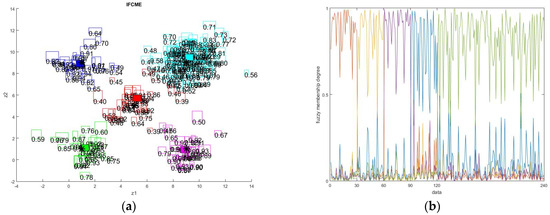
Figure 1.
(a) IFCME clustering results and fuzzy membership, and (b) relationship between data and degree of membership.
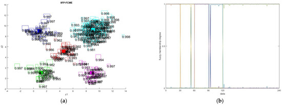
Figure 2.
(a) IIFPFCME clustering results and fuzzy membership, and (b) relationship between data and degree of membership.
Hence, the contributions in this paper are two fuzzy clustering approaches called the new interval fuzzy partitions fuzzy C-means clustering algorithms that were proposed. The proposed algorithms independently combined Euclidean distance and city block distance to achieve fast convergence. The proposed methods showed a faster convergence speed and better performance results compared to the traditional interval fuzzy c-means clustering method in SIDA. Additionally, symbolic interval data often present a challenge of large and small group division, which was also addressed using the proposed methods. Additionally, the IFPFCM algorithm was introduced to handle outliers through interval distance measurement. The experimental comparative analysis revealed that the IFPFCM clustering algorithm with the city block distance measure was suitable for dealing with SIDA with outliers. Finally, this study tested nine groups of data, and the statistical results demonstrated that the proposed algorithm outperformed the traditional method in terms of convergence and efficiency.
The organization of the rest of this paper is as follows. In Section 2, backgrounds on definition and distance measures for interval data are detailed. In Section 3, an improved fuzzy partitions fuzzy C-means clustering algorithm is briefly introduced. In Section 4, two interval improved fuzzy partitions fuzzy C-means clustering algorithms are proposed and discussed. The simulation results are shown in Section 5. Finally, the conclusions are summarized in Section 6.
2. Definition and Distance Measures for Symbolic Interval Data
In this paper, the definition of an interval was outlined as the lower and upper bounds. If it was on the line, it was expressed as , where . When we represent data in multiple intervals, it can be expressed as the following: let and be two interval datasets, where and indicate the values of the interval for the [30].
The first distance measure is termed the L1 norm, or city block distance [31]. The representation in the interval is the sum of the absolute values of the differences in all intervals:
The second is called the L2 norm, or Euclidean distance [32]; the representation in the interval is the sum of the square roots of the differences in all intervals:
Figure 3 shows the relationship between city block distance and Euclidean distance under the center point in 2-dimensional space. The equidistant distance between the city block distance and the center point is similar to the rhombus in Figure 3 with the black line. Moreover, the Euclidean distance was equidistant from the center point according to the Pythagorean theorem, which is similar to a circle shape with a red line [37].
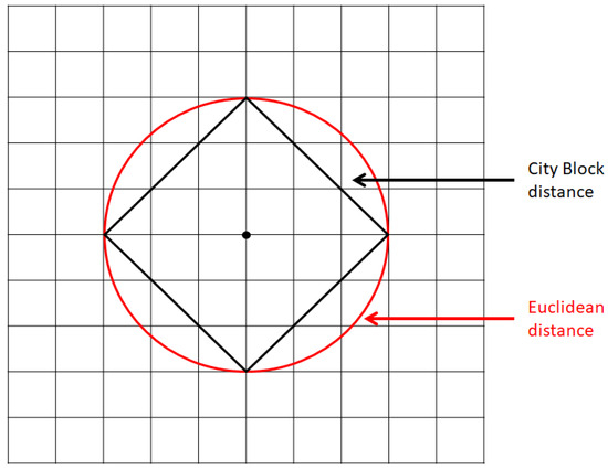
Figure 3.
The relationship between city block distance and Euclidean distance and the center point in 2-dimensional space.
It can be seen from Figure 3 that different distance measures have different characteristics for different sets of data, and we discussed these differences in the experimental results section.
3. Improved Fuzzy Partitions Fuzzy C-Means Clustering Algorithm
In this section, the IFPFCM clustering algorithm has been briefly reviewed. It considers rewarding more crisp membership degrees. By adding the second term, when the degree of membership becomes fuzzier, the increase in the second term can minimize Equation (3) and use this to reward the degree of membership, making it more clearly divided. From Equation (3), a second term was evaluated as ; if the membership degrees become fuzzier, the second term increases the “reward” term for membership degrees near 0 and 1 in order to force a more crisply assignment. Since we sought to minimize Equation (4), this modification rewards crisp membership degrees. The IFPFCM clustering algorithm is used in Lagrangian theory to minimize the objective function , as shown in Equation (3), and the constraints are in Equation (4). The IFPFCM clustering algorithm has two updated equations for and , which are outlined in Equations (5) and (6), respectively [29]:
where denotes the fuzzy membership degree, is a matrix, is th data of the dataset, is the th prototype of the prototype matrix, and is the distance measure between and . As always remains positive, the maximal reward following is denoted in the following equation:
4. Interval Improved Fuzzy Partitions Fuzzy C-Means Clustering Algorithm
The new objective function was proposed to extend the IFPFCM clustering algorithm so that interval data can be processed in this paper. The proposed method combines the advantages of the IFPFCM clustering algorithm, rewarding crisp membership degrees, and the characteristics of fast convergence. However, the proposed method under Euclidean distance will still be affected by outliers. In order to overcome this shortcoming, adding interval city block distance to the proposed method overcame this problem. The derivation of the IIFPFCM clustering algorithm under Euclidean distance has been proposed in Section 4.1. The derivation of the IIFPFCM clustering algorithm under city block distance has been proposed in Section 4.2.
4.1. Interval Improved Fuzzy Partitions Fuzzy C-Means under Euclidean Distance
The new objective function, , for the IIFPFCM clustering algorithm is based on a squared Euclidean distance between the vectors of intervals given in Equation (8) and of which the constraints are given in Equation (9):
In Equation (8), is the fuzzy membership degree of pattern in the th cluster, and is a matrix; the is similar to the IFPFCM defined in Equation (10):
Using the Lagrange multipliers method for the objective function , the nonlinear unconstraint optimization can be obtained as:
The was considered for the minimum problem; to derive an updated equation for the fuzzy membership degree, can be solved as follows:
for and Thus, Equation (12) can be rewritten as:
for and Substituting Equation (13) into Equation (9) is obtained as:
According to Equations (13) and (14), the updated equation for the fuzzy membership degree is:
for and .
The prototype of the th cluster, which minimizes the objective function , has the bounds of the interval Hence, the updated formula for the prototype accords to the following:
for and Thus, Equation (16) can be rewritten as:
In Equation (8), adding a second term evaluates to . When membership degrees become fuzzier, the second term increases as a ‘reward’ for membership degrees near 0 and 1, aiming to enforce a crisper assignment. The adoption of this concept accelerates the convergence of IIFPFCME in this study. By introducing the second term, as membership degrees become fuzzier, its increase can minimize Equation (8). This effectively rewards the degree of membership, resulting in clearer divisions.
4.2. Interval Improved Fuzzy Partitions Fuzzy C-Means under City Block Distance
The new objective function, , for the IIFPFCM clustering algorithm is based on a city block distance between the vectors of intervals given in Equation (18) and of which the constraints are given in Equation (19):
In Equation (18), is the fuzzy membership degree of pattern in the th cluster, and is a matrix; the is similar to the IFPFCM defined in Equation (20):
Using the Lagrange multipliers method for the objective function , the nonlinear unconstraint optimization can be obtained as:
The was considered for the minimum problem; to obtain an updated equation of the fuzzy membership degree, can be solved as followed:
for and Thus, Equation (22) can be rewritten as:
for and Substituting Equation (23) into Equation (19) is obtained as:
According to Equations (23) and (24), the updated equation for the fuzzy membership degree is:
for and .
The prototype of the th cluster, which minimizes the objective function has the bounds of the interval , which was updated according to the following problem:
This yields two well-known minimization problems in norm, such as:
In De Carvalho et al., 2006 [32], the solutions of minimized for have been shown as the median of set { for }. In De Carvalho et al., 2006 [32], there was no in the objection function. However, in this paper, we needed to consider . Hence, we needed to consider that if , then , and if , then . This criteria for the fuzzy membership degree represented by it is greater than the average of all groups, so the degree is strengthened, making its grouping more obvious. As a result, the updated equations of and are obtained as:
where and denote the medians of sets {, for and } and {, for and }, respectively.
The proposed IIFPFCM under city block distance (IIFPFCMC) clustering algorithm used the median instead of the average to update the center point of the group. Hence, the characteristic of the median is that if there are extreme values such as outliers, it can better centralize the trend, and the average will affect affected by extreme values. Hence, when the interval data have outliers, the proposed IIFPFCMC clustering algorithm can effectively avoid being affected at the center point of the update group; that is, the proposed IIFPFCMC used Equations (26)–(28) to update the center point of the cluster and used the median value instead of the mean value. Usually, the characteristic of the median is that if there are extreme values, it can better centralize the tendency. However, the average will be affected by the extreme values. Therefore, when the data have outliers, using the median calculation at the center point of the update group can effective avoid the influence of outliers. Usually, the proposed IIFPFCMC clustering algorithm directly using the median is easily affected by the center point of the initial value, resulting in the situation that the center point of the cluster appears in the same group. Therefore, we separated the initial group center points with IIFPFCME, and then used the algorithm of the median for the IIFPFCMC clustering algorithm, which makes it easier to have a good convergence effect with modified Equations (26)–(28) in this paper. Algorithm 1 presents the procedures of the proposed IIFPFCME clustering algorithm with Euclidean distance. Algorithm 2 presents the procedures of the proposed IIFPFCMC clustering algorithm with city block distance.
| Algorithm 1: Procedures of the proposed IIFPFCME clustering algorithm in the following steps |
| Step 1: Initialization fix ; fix ; fix ; Set iteration counter and iteration limit ; Initialization . |
| Step 2: Update the and . |
| Step 3: Update the . |
| Step 4: Update the . |
| Step 5: if ( or ) Stop. Else and go to Step 2. |
| Algorithm 2: Procedures of the proposed IIFPFCMC clustering algorithm in the following steps |
| Step 1: Initialization fix ; fix ; fix ; Set iteration counter and iteration limit ; Initialization . |
| Step 2: Update the and . |
| Step 3: Update the . |
| Step 4: Update the . |
| Step 5: If ( or ) Stop. Else and go to Step 2. |
5. Simulation Results
We compared five approaches, namely IFCME, IFCMC, IPFCME, IIFPFCME, and IIFPFCMC with IDS1–2 datasets and IFCME, IFCMC, IIFPFCME, and IIFPFCMC with IDS1–6 datasets that have several datasets that include outlier interference. We also presented two real datasets concerning exchange rates for validation of the proposed methods. For a detailed description of the datasets used in this paper, please refer to [34,35]. For all datasets, we used the following computational protocols: stop requirement = 0.00001, and iteration limit = 300. All experiments were run on a computer with Intel(R) Xeon(R) CPU E3-1231 v3 @ 3.40 GH, 32 GB memory, Microsoft Windows 10, and MATLAB 2018b. The performance using the root-mean-square error (RMSE) to computer the true cluster center and corresponding cluster center is defined as:
where is the true cluster center and is the corresponding cluster center.
The first dataset (DS1) consists of five clusters in 2D space which satisfy the standard normal distributions, whose centers are (1, 1), (1, 9), (9, 1), (5, 5), and (9, 9). For the first four clusters, the number of data points per cluster was 30, and their respective covariance matrices were . For the last cluster centered at (9, 9), there were 120 data points, and their covariance matrix was . These data are shown in Figure 4a. In order to build the interval data (symbolic) sets, this was defined as , from which and were drawn randomly from [0.2, 1], as shown in Figure 4b.
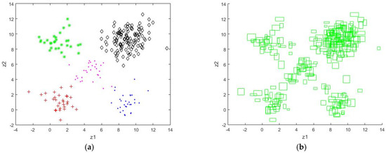
Figure 4.
(a) The first dataset (DS1) and (b) interval datasets of DS1 (IDS1).
The results of IFCME and IFCMC with for IDS1 are shown in Figure 5, where * is the true cluster center; the same color denotes the same clustering (group), and the symbol data with a fill-in color on each color (clustering) is the cluster center of results. The results of IIFPFCME and IIFPFCMC with parameters and for IDS1 are shown in Figure 6 and Figure 7, respectively. The results of IPFCME for IDS1 are shown in Figure 8. There are three indexes: the RMSE, the average usage time of ten times, and the average of ten iterations as a comparison on Table 1, Table 2, Table 3, Table 4, Table 5 and Table 6. The results of the comparison are shown in Table 1. From Table 1, the proposed IIFPFCME and IIFPFCMC on performance and average times all are better than IFCME, IFCMC, and IPFCME. From Table 1, the proposed IIFPFCME appears to be better than the proposed IIFPFCMC under IDS1. IDS1 is a symbolic dataset without outliers. From Figure 5, the clustering results are not good, as the center of the five clusters cannot be found correctly. Hence, we used “---” as the RMSE in Table 1. From Table 1, IPFCME takes more time, but its clustering results are not better than IIFPFCME.
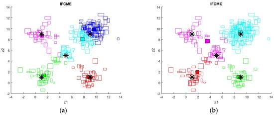
Figure 5.
The results of the (a) IFCME and (b) IFCMC parameters with for IDS1.
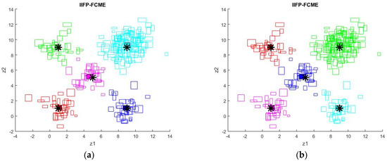
Figure 6.
The results of the IIFPFCME parameter with (a) and (b) for IDS1.
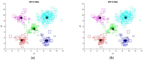
Figure 7.
The results of the IIFPFCMC parameter with (a) and (b) for IDS1.
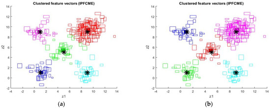
Figure 8.
The results of the IPFCME parameter with (a) and (b) for IDS1.

Table 1.
The results of the comparison for IDS1 with different approaches: (a) using IFCME and IIFPFCME under different ; (b) using IFCMC and IIFPFCMC under different ; and (c) using IPFCME.
Table 2.
The results of the comparison for IDS2 with different approaches: (a) using IFCME and IIFPFCME under different ; (b) using IFCMC and IIFPFCMC under different ; and (c) using IPFCME.
Table 3.
The results of the comparison for IDS3 with different approaches: (a) using IFCME and IIFPFCME under different ; and (b) using IFCMC and IIFPFCMC under different .
Table 4.
The results of the comparison for IDS4 with different approaches: (a) using IFCME and IIFPFCME under different ; and (b) using IFCMC and IIFPFCMC under different .
Table 5.
The results of the comparison for IDS5 with different approaches: (a) using IFCME and IIFPFCME under different ; and (b) using IFCMC and IIFPFCMC under different .
Table 6.
The results of the comparison for IDS6 with different approaches: (a) using IFCME and IIFPFCME under different ; and (b) using IFCMC and IIFPFCMC under different .
The second dataset (DS2) with 243 points was constructed using DS1 and another one-point (14, 4) outlier, as shown in Figure 9a. On the other hand, the interval datasets of DS2 (IDS2) are shown in Figure 9b. In this case, the symbolic data with outliers were illustrated as powerful via the proposed IIFPFCMC method.
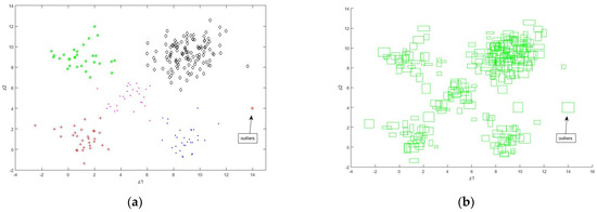
Figure 9.
(a) The second dataset (DS2) and (b) interval datasets of DS2 (IDS2).
The results of IFCME and IFCMC with for IDS2 are shown in Figure 10. The results of IIFPFCME and IIFPFCMC with parameters and for IDS2 are shown in Figure 11 and Figure 12, respectively. The results of IPFCME for IDS2 are shown in Figure 13. The results of the comparison are shown in Table 2. From Table 2, the proposed IIFPFCME and IIFPFCMC on performance and average times are all better than IFCME, IFCMC, and IPFCME. From Table 2, the proposed IIFPFCMC is better than the proposed IIFPFCME under a symbolic set with outliers. From Figure 10, the clustering results are not good, as the center of the five clusters cannot be found correctly. Hence, we used “---” as the RMSE in Table 2. From Table 2, IPFCME takes more time, but its clustering results are not better than IIFPFCME.
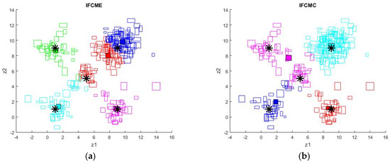
Figure 10.
The results of the (a) IFCME and (b) IFCMC parameters with for IDS2.
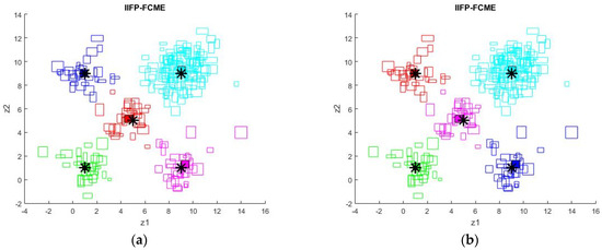
Figure 11.
The results of the IIFPFCME parameter with (a) and (b) for IDS2.
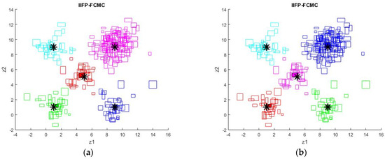
Figure 12.
The results of the IIFPFCMC parameter with (a) and (b) for IDS2.
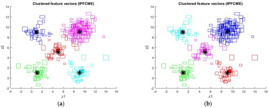
Figure 13.
The results of the IPFCME parameter with (a) and (b) for IDS2.
The third dataset (DS3) with 252 points was constructed using DS1 and added four points, namely (14, 6), (6, 14), (6, −4), and (−4, 6), as shown in Figure 14a. On the other hand, the interval datasets of DS3 (IDS3) are shown in Figure 14b. In this case, the symbolic data with more outliers and different positions were illustrated as powerful via the proposed IIFPFCMC method. Additionally, due to IPFCME in Table 1 and Table 2 on the RMSE and average times, the results were worse than the proposed methods. Therefore, the following examples were not presented in the table.
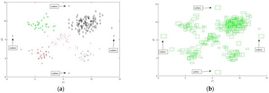
Figure 14.
(a) The third dataset (DS3) and (b) interval datasets of DS3 (IDS3).
The results of IFCME and IFCMC with parameter for IDS3 are shown in Figure 15. The results of IIFPFCME and IIFPFCMC with parameters and for IDS3 are shown in Figure 16 and Figure 17, respectively. The results of the comparison are shown in Table 3. From Table 3, the proposed IIFPFCME and IIFPFCMC on performance and average times are all better than IFCME, IFCMC, and IPFCME. From Table 3, the proposed IIFPFCMC is better than the proposed IIFPFCME under a symbolic set with more outliers and different positions.
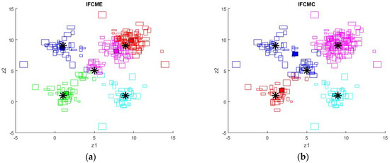
Figure 15.
The results of the (a) IFCME and (b) IFCMC parameters with for IDS3.
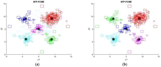
Figure 16.
The results of the IIFPFCME parameter with (a) and (b) for IDS3.
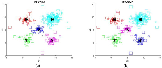
Figure 17.
The results of the IIFPFCMC parameter with (a) and (b) for IDS3.
The fourth dataset (DS4) with 249 points consists of five clusters whose centers are (1, 1), (1, 9), (9, 1), (5, 5), and (9, 9) and diamond shapes on each group. For the first four clusters, the number of data points per cluster was 41 data points. For the last cluster centered at (9, 9), there were 85 data points (see Figure 18a); that is, DS4 used large and small groups and diamond shapes on each group to demonstrate the advantages of the proposed method. In order to build the interval datasets, this was defined as , from which and were drawn randomly from [0.2, 1] (see Figure 18b).
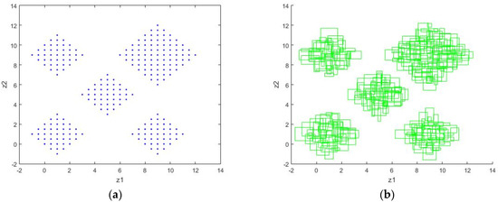
Figure 18.
(a) The fourth dataset (DS4) and (b) interval datasets of DS4 (IDS4).
The results of IFCME and IFCMC with parameter for IDS4 are shown Figure 19. The results of IIFPFCME and IIFPFCMC with parameters and for IDS4 are shown Figure 20 and Figure 21, respectively. Table 4 shows the results of the comparison for IDS4 with different approaches, namely IFCME, IIFPFCME under different , IFCM, and IIFPFCMC under different From Table 4, the proposed IIFPFCME and IIFPFCMC on performance and average times are all better than IFCME and IFCMC. From Table 4, the proposed IIFPFCMC is better than the proposed IIFPFCME under a symbolic set of large and small groups and diamond shapes on each group on the RMSE.
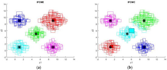
Figure 19.
The results of the (a) IFCME and (b) IFCMC parameters with for IDS4.
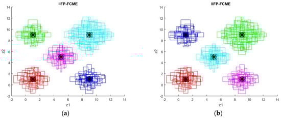
Figure 20.
The results of the IIFPFCME parameter with (a) and (b) for IDS4.
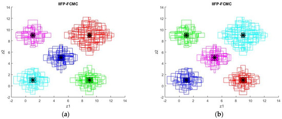
Figure 21.
The results of the IIFPFCMC parameter with (a) and (b) for IDS4.
The fifth dataset (DS5) with 252 points were constructed using DS4 and another one-point (14, 4) outlier, as shown as Figure 22a. On the other hand, the interval datasets of DS5 (IDS5) are shown in Figure 22b; that is, IDS5 used large and small groups, outliers, and diamond shapes on each group to demonstrate the advantages of the proposed method.
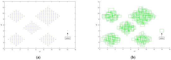
Figure 22.
(a) The fifth dataset (DS5) and (b) interval datasets of DS5 (IDS5).
The results of IFCME and IFCMC with parameter for IDS5 are shown in Figure 23. The results of IIFPFCME and IIFPFCMC with parameters and for IDS5 are shown in Figure 24 and Figure 25, respectively. Table 5 shows the results of the comparison for IDS5 with different approaches, namely IFCME, IIFPFCME under different , IFCMC, and IIFPFCMC under different From Table 5, the proposed IIFPFCME and IIFPFCMC on performance and average times are all better than IFCME and IFCMC. From Table 5, the proposed IIFPFCMC is better than the proposed IIFPFCME under a symbolic set of large and small groups, outliers, and diamond shapes on each group on the RMSE.
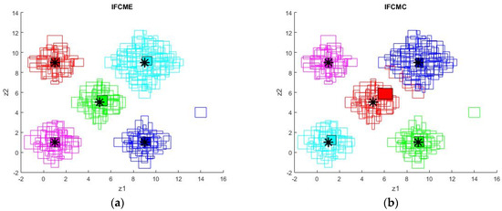
Figure 23.
The results of the (a) IFCME and (b) IFCMC parameters with for IDS5.
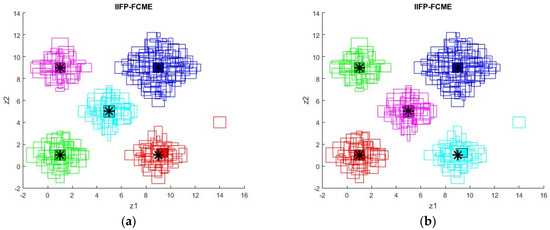
Figure 24.
The results of the IIFPFCME parameter with (a) and (b) for IDS5.
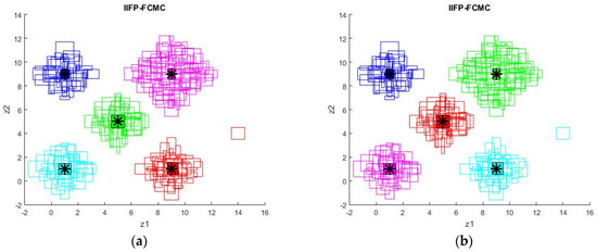
Figure 25.
The results of the IIFPFCMC parameter with (a) and (b) for IDS5.
The sixth dataset (DS6) with 261 points were constructed using DS4 and added four points, namely (14, 6), (6, 14), (6, −4), and (−4, 6), as shown as Figure 26a. On the other hand, the interval datasets of DS6 (IDS6) are shown in Figure 26b. That is, IDS6 used large and small groups, more outliers, and diamond shapes on each group to demonstrate the advantages of the proposed method.
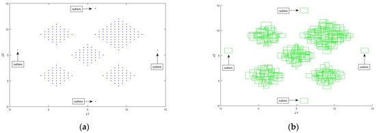
Figure 26.
(a) The sixth dataset (DS6) and (b) interval datasets of DS6 (IDS6).
The results of IFCME and IFCMC with parameter for IDS6 are shown in Figure 27. The results of IIFPFCME and IIFPFCMC with parameters and for IDS6 are shown in Figure 28 and Figure 29, respectively. Table 6 shows the results of the comparison for IDS6 with different approaches, namely, IFCME, IIFPFCME under different , IFCMC, and IIFPFCMC under different From Table 6, the proposed IIFPFCME and IIFPFCMC on performance and average times are all better than IFCME and IFCMC. From Table 6, the proposed IIFPFCMC is better than the proposed IIFPFCME under a symbolic set of large and small groups, more outliers, and diamond shapes on each group on the RMSE.
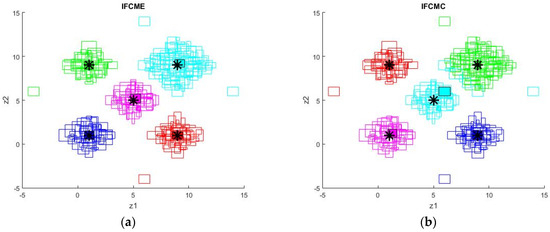
Figure 27.
The results of the (a) IFCME and (b) IFCMC parameters with for IDS6.
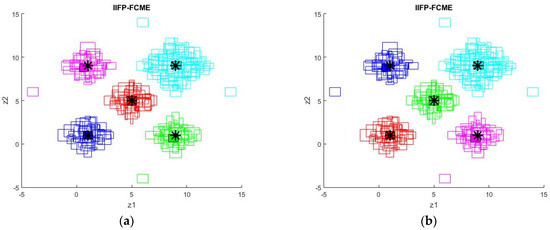
Figure 28.
The results of the IIFPFCME parameter with (a) and (b) for IDS6.
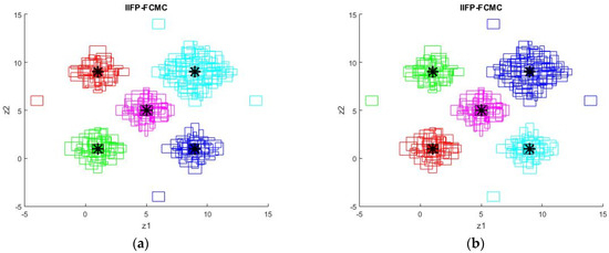
Figure 29.
The results of the IIFPFCMC parameter with (a) and (b) for IDS6.
We presented two real datasets concerning exchange rates for validation of the proposed methods. The seventh interval dataset (IDS7) represents weekly low- and high-price correlation data for EUR/USD on z2 and TW/USD on z1. The eighth interval dataset (IDS8) represents weekly low- and high-price correlation data for GBP/USD on z2 and TW/USD on z1. For the currency exchange rate dataset, data were collected during a 5-year period (2011–2015). For a detailed description of this dataset on currency exchange rates and the results of IFCME, please refer to the study published by the authors of [35].
The results of IFCMC with parameter for IDS7 are shown in Figure 30a. The results of IIFPFCMC and IIFPFCME with parameters , and for IDS7 are shown in Figure 30b–d and Figure 31 respectively. Table 7 shows the results of the comparison for IDS7 with different approaches: (a) using IFCME and IIFPFCME under different ; and (b) using IFCMC and IIFPFCMC under different . From Table 7, the proposed IIFPFCME and IIFPFCMC appear better than the IFCME and IFCMC, respectively. Note that due to it being a real dataset, there is no information regarding the cluster center; the results only show the comparison on average times on ten (sec.) and average number of ten iterations () and no RMSE in the table.
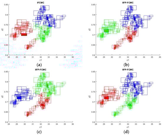
Figure 30.
The results of IFCMC. (a) The results of the IIFPFCME parameter with (b) (c) , and (d) for IDS7.
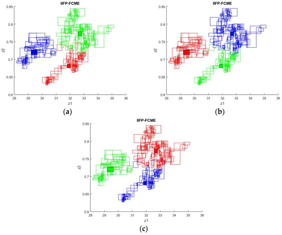
Figure 31.
The results of the IIFPFCME parameter with (a) (b) , and (c) for IDS7.
Table 7.
The results of the comparison for IDS7 with different approaches: (a) using IFCME and IIFPFCME under different ; and (b) using IFCMC and IIFPFCMC under different .
The results of IFCMC with parameter for IDS8 are shown in Figure 32a. The results of IIFPFCMC and IIFPFCME with parameters , and for IDS7 are shown in Figure 32b–d and Figure 33, respectively. Table 8 shows the results of the comparison for IDS7 with different approaches: (a) using IFCME and IIFPFCME under different ; and (b) using IFCMC and IIFPFCMC under different . From Table 8, the proposed IIFPFCME and IIFPFCMC appear better than the IFCME and IFCMC, respectively.
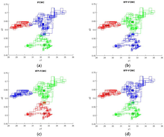
Figure 32.
The results of IFCMC. (a) The results of the IIFPFCME parameter with (b) (c) , and (d) for IDS8.
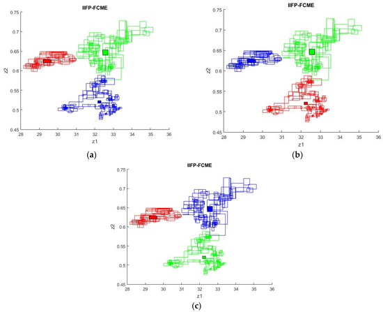
Figure 33.
The results of the IIFPFCME parameter with (a) (b) , and (c) for IDS8.
Table 8.
The results of the comparison for IDS8 with different approaches: (a) using IFCME and IIFPFCME under different ; and (b) using IFCMC and IIFPFCMC under different .
In order to assess the efficiency of the proposed methods, the silhouette index (SI) was used as a clustering validation index. The SI is a metric used to calculate the goodness of a clustering technique. Its value provides a measure of how similar an object is to its own cluster (cohesion) compared to other clusters (separation). The SI is particularly useful under scenarios where the true labels of the data are not known [38,39]. It provides a way to compare the effectiveness of different clustering methods on a given dataset:
where is the mean distance to the points in the same cluster, and is the mean distance to the points in the nearest other cluster. Regarding the interpretation of the SI, (a) the silhouette coefficient ranges from −1 to +1; (b) a high value indicates that the object is well matched to its own cluster and poorly matched to their neighboring clusters. If most objects have a high value, then the clustering configuration is appropriate; (c) if many points have a low or negative value, then the clustering configuration may have too many or too few clusters. Due to IDS7 and IDS8 being real datasets, there is no information regarding their cluster centers. Hence, the SI was used as a clustering validation index to assess the efficiency of the proposed methods. The compared results used the SI of IDS7 with IFCME and the proposed IIFPFCME with different in Table 9. The compared results used the SI of IDS8 with IFCME and the proposed IIFPFCME with different in Table 10. Table 9 and Table 10 show that the proposed methods have good results in terms of efficiency with the SI.
Table 9.
The compared results used the SIs of IDS7–8 with IFCME and the proposed IIFPFCME with different .
Table 10.
The compared results used the SIs of IDS7–8 with IFCMC and the proposed IIFPFCMC with different .
In the above tests, we used three types of data points and added outlier data to these three types for testing. The algorithm of IIFPFCMC exhibits better clustering results in the diamond-shaped and square-shaped distribution data points, and the outlier data were added to these three types of data. The performance and average of ten iterations of the IIFPFCMC algorithm was also found to be better. Although the number of iterations of the proposed IIFPFCMC was reduced, it takes more computing time to obtain the median. The results displayed in all tables were based on converging to the best group center point to count the time and the number of iterations. Hence, the proposed IIFPFCM clustering algorithm with the city block distance measure was deemed to be suitable for dealing with SIDA with outliers and exhibits a better performance and average of iterations than IFCME, IFCMC, and IPFCME. Additionally, the results of the real datasets also indicate that the proposed methods have good results in terms of efficiency with the SI.
6. Conclusions
This study presented the IIFPFCM clustering algorithm, focusing on achieving fast convergence through independent combinations with both Euclidean distance and city block distance. Both proposed methods exhibited faster convergence speeds compared to the traditional IFCM and IPFCM clustering methods in SIDA. Furthermore, there was an issue of partitioning into large and small groups in the context of SID. The proposed methods also yielded superior performance results compared to the traditional IFCM clustering method for addressing this challenge. Additionally, traditional IFCM clustering is susceptible to outliers. This study also introduced the IIFPFCM algorithm, which tackles outliers by employing interval distance measurements. In other words, we enhanced the convergence speed of IFCM, reduced the computation time, and achieved a more effective handling of outliers. In our experiments, we compared three types of data points and introduced outlier data to each of these types. The results of these experiments demonstrated that IIFPFCME effectively enhances convergence speed and the partitioning of data into large and small groups. However, it is worth noting that IIFPFCMC effectively handles outlier data but is sensitive to the choice of initial values in this study. Additionally, the proposed algorithm is currently not affiliated with any commercial entities, and its development remains in the theoretical stage. Regarding the directions for further development of the presented algorithms, SIDA will be employed in many sectors, like healthcare, marketing, education, etc., since SIDA usually provides analysts with a large amount of data on behavior. Moreover, in robotics and autonomous systems, SIDA can aid in interpreting these data for navigation, obstacle avoidance, and decision-making processes. In agriculture, SIDA can aid in soil classification, crop monitoring, and yield prediction by handling the imprecision inherent in agricultural data. In the context of market research, SIDA can be employed to segment markets and understand consumer groups based on imprecise data like survey responses. In bioinformatics, SIDA can assist in grouping similar genetic profiles, which can be useful in understanding diseases and developing treatments.
Author Contributions
Conceptualization, S.-C.C. and J.-T.J.; methodology, S.-C.C. and J.-T.J.; programming, S.-C.C.; writing—original draft preparation, S.-C.C. and J.-T.J.; writing—review and editing, W.-C.C. and J.-T.J.; funding acquisition, J.-T.J. All authors have read and agreed to the published version of the manuscript.
Funding
This work was supported by the National Science Council Under Grant NSTC 110-2221-E-150-040.
Institutional Review Board Statement
Not applicable.
Informed Consent Statement
Not applicable.
Data Availability Statement
The data presented in this study are available in article.
Conflicts of Interest
The authors declare no conflict of interest.
Abbreviations
| DS | Datasets |
| FCM | Fuzzy C-means |
| FMD | Fuzzy membership degree |
| IDS | Interval datasets |
| IFCMC | Interval fuzzy C-means with city block distance |
| IFCME | Interval fuzzy C-means with Euclidean distance |
| IFPFCM | Improved fuzzy partitions for fuzzy regression models |
| IIFPFCM | Interval improved fuzzy partitions fuzzy C-means |
| IIFPFCMC | IIFPFCM with city block distance |
| IIFPFCME | IIFPFCM with Euclidean distance |
| IPFCM | Interval possibilistic FCM |
| PMD | Possibilistic membership degree |
| RMSE | Root-mean-square error |
| SID | Symbolic interval data |
| SIDA | Symbolic interval data analysis |
References
- Billard, L.; Diday, E. Symbolic Data Analysis: Conceptual Statistics and Data Mining; John Wiley & Sons: London, UK, 2006. [Google Scholar]
- Chuang, C.-C.; Jeng, J.-T.; Chang, S.-C. Hausdorff distance measure based interval fuzzy possibilistic c-means clustering algorithm. Int. J. Fuzzy Syst. 2013, 15, 471–479. [Google Scholar]
- He, Q.; He, Z.; Duan, S.; Zhong, Y. Multi-objective interval portfolio optimization modeling and solving for margin trading. Swarm Evol. Comput. 2022, 75, 101141. [Google Scholar] [CrossRef]
- Zhou, B.; Wang, X.; Zhou, J.; Jing, C. Trajectory recovery based on interval forward–backward propagation algorithm fusing multi-source information. Electronics 2022, 11, 3634. [Google Scholar] [CrossRef]
- Yamaka, W.; Phadkantha, R.; Maneejuk, P. A convex combination approach for artificial neural network of interval data. Appl. Sci. 2021, 11, 3997. [Google Scholar] [CrossRef]
- Fordellone, M.; De Benedictis, I.; Bruzzese, D.; Chiodini, P. A maximum-entropy fuzzy clustering approach for cancer detection when data are uncertain. Appl. Sci. 2023, 13, 2191. [Google Scholar] [CrossRef]
- Freitas, W.W.F.; Souza, R.M.C.R.; Getúlio, J.A.; Bastian, F. Exploratory spatial analysis for interval data: A new autocorrelation index with COVID-19 and rent price applications. Expert Syst. Appl. 2022, 195, 116561. [Google Scholar] [CrossRef]
- Chang, W.; Ji, X.; Liu, Y.; Xiao, Y.; Chen, B.; Liu, H.; Zhou, S. Analysis of university students’ behavior based on a fusion k-means clustering algorithm. Appl. Sci. 2020, 10, 6566. [Google Scholar] [CrossRef]
- Zhang, R.-L.; Liu, X.-H. A novel hybrid high-dimensional pso clustering algorithm based on the cloud model and entropy. Appl. Sci. 2023, 13, 1246. [Google Scholar] [CrossRef]
- Dougherty, E.R.; Brun, M. A probabilistic theory of clustering. Pattern Recognit. Soc. 2004, 37, 917–925. [Google Scholar] [CrossRef]
- Volkovich, Z.; Avros, R.; Golani, M. On initialization of the expectation maximization clustering algorithm. Glob. J. Technol. Optim. 2011, 2, 1–4. [Google Scholar]
- Sun, T.; Shu, C.; Li, F.; Yu, H.; Ma, L.; Fang, Y. An efficient hierarchical clustering method for large datasets with map-reduce. In Proceedings of the 2009 International Conference on Parallel and Distributed Computing, Applications and Technologies, Boston, MA, USA, 24–26 September 2009; pp. 494–499. [Google Scholar]
- Li, M.; Deng, S.; Wang, L.; Feng, S.; Fan, J. Hierarchical clustering algorithm for categorical data using a probabilistic rough set model. Knowl. Based Syst. 2014, 65, 60–71. [Google Scholar] [CrossRef]
- Patel, S.; Sihmar, S.; Jatain, A. A study of hierarchical clustering algorithms. In Proceedings of the 2015 2nd International Conference on Computing for Sustainable Global Development (INDIACom), New Delhi, India, 11–13 March 2015; pp. 537–541. [Google Scholar]
- Hartigan, J.A.; Wong, M.A. Algorithm AS 136: A k-means clustering algorithm. J. R. Stat. Soc. Ser. C Appl. Stat. 1979, 28, 100–108. [Google Scholar] [CrossRef]
- Park, H.S.; Jun, C.H. A simple and fast algorithm for K-medoids clustering. Expert Syst. Appl. 2009, 36, 3336–3341. [Google Scholar] [CrossRef]
- Fahad, A.; Alshatri, N.; Tari, Z.; Alamri, A.; Khalil, I.; Zomaya, A.Y.; Foufou, S.; Bouras, A. A survey of clustering algorithms for big data: Taxonomy and empirical analysis. IEEE Trans. Emerg. Top. Comput. 2014, 2, 267–279. [Google Scholar] [CrossRef]
- Bezdek, J.C.; Ehrlich, R.; Full, W. FCM: The fuzzy c-means clustering algorithm. Comput. Geosci. 1984, 10, 191–203. [Google Scholar] [CrossRef]
- Mújica-Vargas, D.; Kinani, J.M.V.; Rubio, J.D. Color-based image segmentation by means of a robust intuitionistic fuzzy c-means algorithm. Int. J. Fuzzy Syst. 2020, 22, 901–916. [Google Scholar] [CrossRef]
- Gao, Y.; Li, H.; Li, J.; Cao, C.; Pan, J. Patch-based fuzzy local weighted c-means clustering algorithm with correntropy induced metric for noise image segmentation. Int. J. Fuzzy Syst. 2023, 25, 1991–2006. [Google Scholar] [CrossRef]
- Hussain, I.; Sinaga, K.P.; Yang, M.-S. Unsupervised multiview fuzzy c-means clustering algorithm. Electronics 2023, 12, 4467. [Google Scholar] [CrossRef]
- Shi, Y. Application of FCM clustering algorithm in digital library management system. Electronics 2022, 11, 3916. [Google Scholar] [CrossRef]
- Tang, Y.; Chen, R.; Xia, B. VSFCM: A novel viewpoint-driven subspace fuzzy c-means algorithm. Appl. Sci. 2023, 13, 6342. [Google Scholar] [CrossRef]
- Wang, Y.; Qin, Q.; Zhou, J.; Chen, Y.; Han, S.; Wang, L.; Du, T.; Ji, K.; Zhao, Y.O.; Zhang, K. Guided filter-based fuzzy clustering for general data analysis. Int. J. Fuzzy Syst. 2023, 25, 2036–2051. [Google Scholar] [CrossRef]
- Sousa, Á.; Silva, O.; Bacelar-Nicolau, L.; Cabral, J.; Bacelar-Nicolau, H. Comparison between two algorithms for computing the weighted generalized affinity coefficient in the case of interval data. Stats 2023, 6, 1082–1094. [Google Scholar] [CrossRef]
- Roh, S.B.; Oh, S.K.; Pedrycz, W.; Wang, Z.; Fu, Z.; Seo, K. Design of iterative fuzzy radial basis function neural networks based on iterative weighted fuzzy c-means clustering and weighted LSE estimation. IEEE Trans. Fuzzy Syst. 2022, 30, 4273–4285. [Google Scholar] [CrossRef]
- Huang, Y.P.; Bhalla, K.; Chu, H.C.; Lin, Y.C.; Kuo, H.C.; Chu, W.J.; Lee, J.H. Wavelet k-means clustering and fuzzy-based method for segmenting MRI images depicting Parkinson’s disease. Int. J. Fuzzy Syst. 2021, 23, 1600–1612. [Google Scholar] [CrossRef]
- Elsheikh, S.; Fish, A.; Zhou, D. Exploiting spatial information to enhance DTI segmentations via spatial fuzzy c-means with covariance matrix data and non-euclidean metrics. Appl. Sci. 2021, 11, 7003. [Google Scholar] [CrossRef]
- Höppner, F.; Klawonn, F. Improved fuzzy partitions for fuzzy regression models. Int. J. Approx. Reason 2003, 32, 85–102. [Google Scholar] [CrossRef]
- Hazarika, I.; Mahanta, A.K. A New Semimetric for Interval Data. Int. J. Recent Technol. Eng. 2019, 8, 3278–3285. [Google Scholar] [CrossRef]
- De Souza, R.M.C.R.; De Carvalho, F.A.T. Clustering of interval data based on city–block distances. Pattern Recognit. Lett. 2004, 25, 353–365. [Google Scholar] [CrossRef]
- De Carvalho, F.D.A.T.; Brito, P.; Bock, H.-H. Dynamic clustering for interval data based on L₂ distance. Comput. Statist. 2006, 21, 231–250. [Google Scholar] [CrossRef]
- Peng, W.; Li, T. Interval Data Clustering with Applications. In Proceedings of the 18th IEEE International Conference on Tools with Artificial Intelligence, Arlington, VA, USA, 13–15 November 2006; pp. 355–362. [Google Scholar]
- De Carvalho, F.D.A.T. Fuzzy c-means clustering methods for symbolic interval data. Pattern Recognit. Lett. 2007, 28, 423–437. [Google Scholar] [CrossRef]
- Jeng, J.-T.; Chen, C.-M.; Chang, S.-C.; Chuang, C.-C. IPFCM clustering algorithm under Euclidean and Hausdorff distance measure for symbolic interval data. Int. J. Fuzzy Syst. 2019, 21, 2102–2119. [Google Scholar] [CrossRef]
- Chen, C.-M.; Chang, S.-C.; Chuang, C.-C.; Jeng, J.-T. Rough IPFCM clustering algorithm and its application on smart phones with Euclidean distance. Appl. Sci. 2022, 12, 5195. [Google Scholar] [CrossRef]
- Kato, J.; Okada, K. Simplification and shift in cognition of political difference: Applying the geometric modeling to the analysis of semantic similarity judgment. PLoS ONE 2011, 6, e20693. [Google Scholar] [CrossRef] [PubMed]
- Rousseeuw, P.J. Silhouettes: A graphical aid to the interpretation and validation of cluster analysis. J. Comput. Appl. Math. 1987, 20, 53–65. [Google Scholar] [CrossRef]
- Shahapure, K.R.; Nicholas, C. Cluster Quality Analysis Using Silhouette Score. In Proceedings of the 2020 IEEE 7th International Conference on Data Science and Advanced Analytics (DSAA), Sydney, NSW, Australia, 6–9 October 2020; pp. 747–748. [Google Scholar]
Disclaimer/Publisher’s Note: The statements, opinions and data contained in all publications are solely those of the individual author(s) and contributor(s) and not of MDPI and/or the editor(s). MDPI and/or the editor(s) disclaim responsibility for any injury to people or property resulting from any ideas, methods, instructions or products referred to in the content. |
© 2023 by the authors. Licensee MDPI, Basel, Switzerland. This article is an open access article distributed under the terms and conditions of the Creative Commons Attribution (CC BY) license (https://creativecommons.org/licenses/by/4.0/).