Abstract
Selective laser melting (SLM) is an additive manufacturing technique commonly used in the rapid prototyping of components. The complexity of the SLM microstructure poses a unique challenge to deriving effective mechanical properties at different length scales. Representative volume elements (RVEs) are often used to homogenize the material properties of composites. Instead of RVEs, we use statistical volume elements (SVEs) to homogenize the elastic and fracture properties of the material. This relates the inherent variation of a material’s microstructure to the variation in its mechanical properties at different observation scales. The convergence to the RVE limit is examined from two perspectives: the stability of the mean value as the SVE size increases for the mean-based approach, and the tendency of the normalized variation in homogenized properties to zero as the SVE size increases for the variation-based approach. Fracture properties tend to make the RVE limit slower than do elastic properties from both perspectives. There are also differences between vertical (normal to printing plane) and horizontal (in-plane) properties. While the elastic properties tend to make the RVE limit faster for the horizontal direction, i.e., having a smaller variation and more stable mean value, the fracture properties exhibit the opposite effect. We attributed these differences to the geometry of the melt pools.
1. Introduction
Selective laser melting (SLM) is an additive manufacturing method where components are formed directly from metal powder [1]. Components formed using SLM are built layer-by-layer using a high-powered laser, localized to a selected area, fusing metallic powder together. This methodology is of particular interest to industries that require complex geometry, or intricate hollow designs [2]. Such complex geometries find value in applications such as aerospace, biomedical and other industries [1]. Considering the diverse applications of components manufactured through SLM, there has been a notable focus on the modeling and simulation aspects.
The area affected by the radiation of the laser can be sectioned into three regions: the fusion zone (FZ), heat-affected zone (HAZ), and substrate [3]. In the fusion zone, metallic powder is briefly liquidized to form pools of melted powder known as melt pools [3]. It is the melt pools, once resolidified, that form the layer-by-layer construction of the SLM component. A 3D conceptual drawing of a melt pool is shown in Figure 1 from [3].
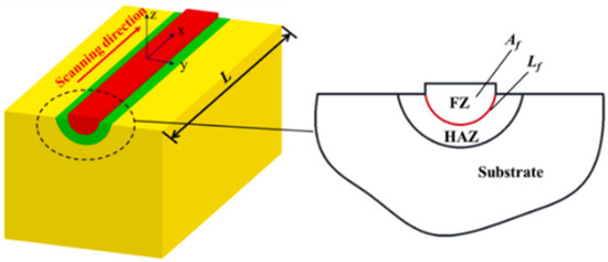
Figure 1.
Conceptual drawing of a melt pool [3].
Melt pool boundaries change size and shape depending on the parameters used in the SLM process, such as laser power and laser scanning speed. These parameters greatly influence induced residual stresses, a hierarchical layout, and the severity of defects such as voids and cracks [4]. The inclusion of melt pools, however, dramatically increases the complexities of the microstructure of SLM materials, making it difficult to establish a correlation between microstructures and mechanical response [5,6,7,8].
Current works have simulated this microstructure using Voronoi tessellation, approximating the polycrystalline geometry of the printed microstructure [5,9,10]. Notably, these studies share a focus on accurately representing the complex microstructural features inherent to AM processes. From [9], a modular methodology is used to obtain representative microstructural cells, encompassing feature-based representations and morphological shape analyses for different AM processes and materials. Analogously, additional works introduce a novel technique that models columnar and equiaxial grains, alongside melt pools, using crystal plasticity and finite element (FE) modeling for SLM components [5]. Additionally, a crystal plasticity-based fast Fourier transform (CP-FFT) framework captures microstructural influences on mechanical responses in SLM-fabricated materials, highlighting the role of grain features [10]. From this perspective, crystal plasticity furnishes the essential microstructural insight required for mechanical analysis, while FFT augments the ability to scrutinize and visualize the spatial distribution of microstructural features.
Other crystal plasticity models are presented in [11], extending the focus to comprehend the impact of crack nucleation behavior on mechanical attributes, specifically the assessment of fatigue life in materials produced through SLM printing. This would suggest that process parameters leading to the formation of different pore types can significantly influence the initiation of fatigue cracks, which directly impacts the mechanical behavior of the material. Moreover, in [12,13], researchers conduct a morphological analysis that directly assesses inherent physical traits, thereby reinforcing the substantial connection between processing parameters and the resulting material behavior.
Even with the extensive literature outlining the effect of various process parameters and demonstrating the effects with approximated domains, there exists a gap in our understanding of the mechanical behavior at different length scales for metal SLM materials. In this work, a framework is introduced to employ a high-fidelity meshing approach to comprehensively represent the intricate complexities of SLM microstructures. Additionally, the variation in mechanical properties is examined across various length scales, elucidating the intricate connection between these fluctuations and specific regions within the melt pool.
Numerical homogenization has proven to be an effective means to quantify material properties, given a microstructure with such complexities [14]. The goal of numerical homogenization is to upscale the effect of all microstructural details into the effective or apparent material properties that can be used in continuum-level models [15]. In homogenization theory, a representative volume element (RVE) refers to a large-enough domain for which a target material property can be considered converged versus the volume element size [16,17,18,19]. There are various perspectives in defining convergence [20,21,22]. For example, one can examine if the given property is almost independent of the choice of boundary conditions used [23,24], whether the mean value has stabilized versus the volume size, or whether the variation of the homogenized properties over a population of volume elements (VEs) of the same size is small enough [25,26]. Depending on the mechanical properties in question, however, constructing an appropriately sized RVE can prove sufficiently challenging, if not impractical [26]. For example, fracture-related properties have very large RVE sizes.
An alternative approach, one that attempts to consider the variability of the microstructure, is the concept of a statistical volume element (SVE), first introduced in [27,28,29] for homogenizing elastic properties. SVE homogenization partitions a large domain into VEs much smaller than the RVE size limit for a given property. Understanding the variation in mechanical properties versus VE (SVE) size and homogenizing properties in terms of SVEs, as opposed to RVEs, has multiple benefits. First, many mechanical properties have a specific form of size effect; that is, the trends in which the mean and variation in the given property change versus the observation (SVE) size [30,31]. Second, RVE-based homogenization has been rendered ineffective in many fracture analyses as all material heterogeneities that play a key role in crack nucleation, propagation, and coalescence are lost in the homogenization process. For example, a lack of convergence or convergence to an incorrect value is reported for fracture pattern [32] and fracture energy [33]. In the method of moving window [34,35], a window (SVE) traverses a macroscopic domain, and each time at the centroid of the SVE assigns the homogenized properties. Unlike RVEs, the homogenized values at different locations are not uniform (or almost uniform), hence the corresponding mesoscopic property fields generated are inhomogeneous and address the aforementioned problem. Third, many interesting mechanical responses of a material are stochastic. For example, for the same sample geometry and loading, different fracture patterns and strain–stress curves are reported in [36] and [37], respectively. The smaller size of SVEs (compared to RVEs) ensures that the homogenized properties are stochastic and maintain the mentioned sample-to-sample variation. In short, the SVE-based properties maintain a certain level of material heterogeneity and randomness, and are a promising tool in multiscale material modeling. For this purpose, the size of SVE can be viewed as the resolution of the homogenization scheme and acts as a gauge between RVE-based homogenization and direction numerical simulation (DNS) in terms of accuracy and efficiency.
The intent of this work is to explore the effects of SVE size against published experimental results of elastic and fracture properties of SLM material and explore the size effect of these properties. The SVE-based homogenization will also examine the effect of the geometry of the melt pools and their intrinsic length scale on homogenized properties at different sizes. Investigating the correlation between microstructure and mechanical properties can prove instrumental in establishing fundamental relationships that govern a material’s behavior.
2. Materials and Methods
The layer-by-layer construction, shown in Figure 2, depicts rows of melt pools atop one another to form the microstructure typical of an SLM material. Consider the cross-section shown in Figure 2 from [38] of an SLM material, referred to as the RVE from hereon.
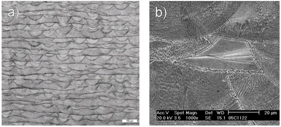
Figure 2.
(a) SEM image of SLM material [38]; (b) enlarged image of a region from (a).
The FE mesh used in this analysis was constructed using the conforming to interface structured adaptive mesh refinement (CISAMR) [39,40] method. The CISAMR is a non-iterative mesh generation algorithm that transforms an initial structured mesh comprising rectangular elements in a high-quality hybrid conforming mesh consisting of rectangular and triangular elements. The meshing process involves three phases: (1) h-adaptive refinement of background elements intersecting material interfaces to minimize the geometric discretization error and accurately approximate stress concentrations in the regions; (2) performing r-adaptivity on the nodes of refined elements cut by material interfaces, which on average transforms 50% of these elements into conforming elements; and (3) the sub-triangulation of the remaining non-conforming elements with hanging nodes, as well as elements with hanging nodes that are created during the h-adaptive refinement phase. The effect of each phase of the CISAMR algorithm on the transformation of a structured mesh into a conforming mesh is visualized in Figure 3 for a smooth interface (see [39] for more algorithmic and implementation details).
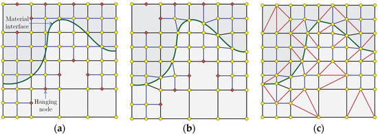
Figure 3.
Transformation of a structured mesh composed of 4-node quadrilateral elements into a conforming mesh using the CISAMR algorithm: (a) h-adaptive refinement in the vicinity of material interfaces; (b) r- adaptivity of the nodes of elements intersecting each interface; (c) sub-triangulating the elements deformed during the r-adaptivity process, as well as elements with hanging nodes created after h-adaptivity. Red, and yellow nodes correspond to hanging nodes created during the SAMR process, and conforming background mesh nodes, respectively.
A unique feature of CISAMR is the ability to generate high-quality meshes for problems with complex morphologies [41]. However, the presence of sharp geometrical features in the microstructure requires the addition of new algorithmic features to the CISAMR algorithm. As shown in Figure 4, in such cases, after the h-adaptivity (SAMR) phase, we first identify all background mesh elements containing sharp corners of melt pools. Next, the closest mesh node to the sharp corner within this element is identified and snapped to the sharp corner. The subsequent phases of the CISAMR algorithm (r-adaptivity and sub-triangulation) are then carried out in the same way as described earlier. With this simple modification, we can enable the CISAMR algorithm to preserve sharp features in the resulting mesh. To mesh the microstructure shown in Figure 2a, we first generate segregated meshes for each melt pool using the modified CISAMR algorithm, and then stitch them together (merge node IDs along their boundaries) to generate the conforming mesh for the entire microstructure.
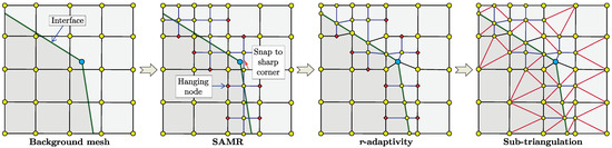
Figure 4.
Modifications in the original CISAMR algorithm to handle the presence of sharp corners along material interfaces. Blue, red, and yellow nodes correspond to sharp corners of the material interface, hanging nodes created during the SAMR process, and conforming background mesh nodes, respectively.
Figure 5a shows the geometrical model constructed for the 924 μm × 840 μm RVE image shown in Figure 2a, in which melt pool boundaries are characterized using non-uniform rational B-splines (NURBS) curves. This domain comprises 239 melt pools and is discretized using the CISAMR algorithms, resulting in a conforming mesh consisting of 1.31 million elements and a maximum aspect ratio of 4.4. The RVE mesh is then partitioned into several smaller SVEs. Four different SVE sizes are analyzed in this work, i.e., 56, 84, 112, and 140 μm. These sizes correspond to 240, 110, 56, and 36 SVE counts, respectively.
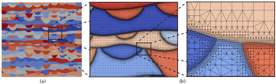
Figure 5.
(a) The microstructure of the SLM material. Each color representing a unique melt pool; (b) a sample SVE extracted from CISAMR mesh generated on the domain in (a), with an inset showing the mesh structure.
Since the RVE mesh contains 239 melt pools, the smallest to largest SVEs contain an average of about 1, 2.2, 4.2, and 6.6 melt pools in each SVE. Accordingly, 56 is the minimum size below which there will be less than one melt pool on average within a SVE. As a sub-melt pool length scale, the model ideally should incorporate grain-level mechanisms, crystal plasticity, or other alternative physics-based models more appropriate for investigating the failure response of the SVE. In the following, we use a cohesive model to model failure between the melt pools. Accordingly, due to the lack of more accurate grain-scale models in this work, we limited the smallest SVE size to 56. As for the largest size, SVEs larger than 140 μm would result in fewer than 36 SVEs, which may be a too small number to accurately calculate the mean and standard deviation of homogenized properties. We refer the reader to [26] on why this is especially a concern for fracture properties due to their slower convergence relative to compared with that of elastic properties. In short, while ideally we could model larger SVEs (if starting with a larger experimental image, as shown in Figure 2a), the chosen sizes still manifest distinct mechanical behaviors. Larger sizes are valuable for revealing interactions between multiple melt pools, while mid-range sizes shed light on interactions between select boundaries.
The microstructure and the corresponding conforming mesh for one of the SVEs with 140 μm are illustrated in Figure 5b. For reference, the CISAMR mesh is generated on a background structured mesh with an element size of 2.8 μm, with two levels of h-adaptive refinement along melt pool boundaries. Accordingly, the SVEs of sizes 56, 84, 112, and 140 μm correspond to 20, 30, 40, and 50 background elements along the edge, respectively. The calibration of material and interface properties and finite element analysis of the SVEs are discussed next.
Finite element analysis by Abaqus [42] was used to analyze the derived SVEs under three different load cases to characterize the response for tensile loading in vertical and horizontal directions (denoted by and subscripts), and shear loading. The most common boundary conditions (BCs) for the homogenization of elastic properties are the kinematic uniform boundary condition (KUBC) and stress uniform boundary condition (SUBC). In the KUBC, two displacements of the boundary nodes are specified as consistent with a macroscopic strain tensor. In the SUBC, traction values corresponding to a constant macroscopic stress tensor are applied on the boundary of VE. KUBC and SUBC provide the upper and lower limits for the homogenized elastic properties, with the properties converging to unique values as the SVE size increases [43,44,45]. The KUBC is not appropriate for the nonlinear failure problem as it does not permit a crack to completely tear vertically or horizontally through the domain. The SUBC is also not appropriate for failure simulations as it cannot model the unloading portion of the homogenized strain-stress response. We have used a mixed boundary condition (MBC) [26] for homogenization. The MBC condition is preferred over the KUBC and SUBC for multiple reasons. First, the homogenized elastic properties are in between the KUBC and SUBC values and thus are not overly over- or under-estimated for small SVE sizes. Second, it allows cracks to completely go through the VE and can model the unloading portion of the strain–stress response, and the problems of KUBC and SUBC, respectively.
To apply the MBC for the tensile loading in the horizontal direction, the top and bottom sides of the SVE are modeled as rollers (zero tangential traction and normal direction), whereas the left and right sides are gradually taken apart by applying opposing spatially uniform and temporally increasing displacement values across all nodes. The terminal value of the applied displacement of SVEs in the horizontal direction is chosen to be large enough so that most SVEs undergo failure through the loading process. For the tangential direction, zero traction is specified for these sides too. We refer the reviewer to [26] for a more thorough description of the MBC and its comparison with the KUBC and SUBC.
The average strains and stresses of the SVEs were computed using a Python script. With the average stresses and strains of the three load cases, the elasticity stiffness was computed using the process described in [26]. The compliance matrix was computed as the inverse of the stiffness matrix. Finally, the vertical and horizontal elastic moduli, denoted by and , were computed from the compliance matrix.
To establish an effective failure model for each SVE, one must consider the interaction between each melt pool, i.e., the boundary between melt pools in Figure 5a (corresponding to melt pools in Figure 2a). Since the fusion zone is melted and deposited on top of the heat-affected zone, there must exist an interface between the two [3]. Several works including [5,9,10] treat such melt pool boundaries as weak interfaces, whose failure response is represented by a cohesive traction–separation relation (TSR).
Figure 6 shows the bilinear TSR used for this study. This TSR is characterized by the initial tangent modulus, , strength value, , and the work of separation (fracture energy), , which is the area under the traction–separation relation.
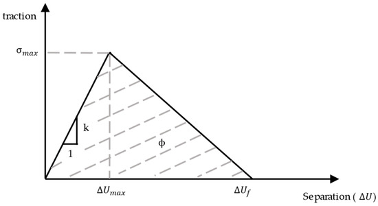
Figure 6.
Bilinear traction separation relation (TSR) modified from [42].
Table 1 shows experimentally measured vertical and horizontal elastic moduli and strengths for the sample shown in Figure 2a from [38]. Our objective is to calibrate the elastic and fracture properties of SLM at the melt pool scale, e.g., bulk properties and melt pool boundary TSR parameters, so that the computationally homogenized elastic and fracture properties for the RVE match the results shown in this table. The last two columns of the table show our computational results for a domain that is half the size of the domain shown in Figure 5a in each direction. As evident, there is a good match between experimental and computational elastic and fracture properties. The details of the calibration process are provided below. Since the experimentally reported stiffnesses and strengths are in GPa and the RVE size in Figure 2a is expressed in μm, we use GPa and μm as units of stiffness/ strength and length for the remainder of the paper.

Table 1.
Experimental results compared to simulation results for vertical and horizontal load cases.
For multiphase composites, the volume fractions and topologies of individual phases contribute to the overall elastic and fracture properties of the material at a given SVE (observation) size. Herein, similar to [5,9,10], the additively manufactured material is treated as single-phase with the melt pool boundaries being the dominant feature responsible for a material nonlinear response. From this perspective, there are two aspects that contribute to the compliance of SLM material: bulk compliance and traction separation model compliance. This is due to the fact that the cohesive model is intrinsic; that is, it has the initial slope of in Figure 6. To demonstrate the effect of cohesive model compliance, consider a one-dimensional domain, wherein equal length elastic regions of length and elastic modulus are separated by cohesive interfaces with initial stiffness . The compliances of the bulk and cohesive interfaces are and , respectively, resulting in the overall compliance,
where is the effective elastic modulus of the material. Clearly, and are effective and bulk compliances. To relate this simple 1D model to the microstructure shown in Figure 2a and Figure 5a, is set to the average spacing of the melt pools in the vertical direction. Subsequently, can be considered to be the elastic modulus of the bulk material within the melt pools. Finally, corresponds to the vertical stiffness of SLM from Table 1 (160.80 GPa). We note that Equation (1) will be exact for the vertical stiffness of material only if in Figure 2a, the melt pool lines are horizontal lines separated by distance . However, this equation still provides a good starting point for choosing the combinations of the bulk material stiffness, , and cohesive model stiffness, , that result in a vertical stiffness close to the experimental value of 160 GPa in Table 1.
Interestingly, the 1D equation relating has worked well in the calibration process by varying , calculating from (1), and assigning reasonable values for and , the other two parameters of the TSR in Figure 6. Specifically, we choose a value of equal to the macroscopic vertical strength of the bulk material equal to 1.08 GPa in Table 1. Unfortunately, no energy measure was provided in the experimental results of [38]; thus, there is no direct means to assign the value of . However, computational results provided some guidance on choosing a reasonable value for ; in Figure 6, the area under the unloading line represents the energy reserve past the maximum strength of the interface; the smaller is defined as the ratio of the unloading to loading energies, the more brittle the behavior of the TSR is. From the simulation of SVEs of different sizes, we encountered nonconvergence problems when 2.
In short, in the calibration process, we only varied the value of , with the corresponding value of obtained from Equation (1), = 1.08 GPa and obtained from 2. Figure 7a,b show the computed vertical stiffness, , and strength, , as a function of . Interestingly, for the same value of 72 GPa/μm, the vertical and from Table 1 are matched simultaneously. Having chosen 72 GPa/μm, other parameters are obtained from the process explained earlier and are reported in Table 2, noting that GPa-μm is the rounded-up fracture energy corresponding to 2, and a Poisson ratio of is a typical value chosen for steel.
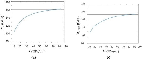
Figure 7.
Calibration of cohesive model stiffness : (a) vertical elastic modulus ; (b) vertical yield (max) stress as a function of .
Table 2.
Material properties set from the calibration process.
Figure 8a shows the VE geometry and boundary conditions used to calibrate the material properties discussed above. Displacement boundary conditions were applied to the top of the domain with a fixed BC at the bottom. Traction-free BCs are used on the left and right sides to match the experimental setup. The corresponding vertical stress vs. strain response is depicted in Figure 8b for the final calibrated parameters. The slope of the linear part matches and the maximum strength matches in Table 1 from [38] (see the last two columns).
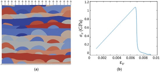
Figure 8.
(a) Domain and boundary condition for vertical loading for parameter calibration; (b) vertical stress versus strain for the domain in (a) with calibrated parameters.
For large enough domains such as the one shown in Figure 8a, the material fails across the boundaries between the melt pools. However, for smaller domains, like the partitioned SVEs, the likelihood of a melt pool boundary permeating across the domain, thus resulting in cohesive fracture along the corresponding TSR interfaces, significantly reduces. As a result, realistically, other modes of material degradation must be included to handle the failure of small SVEs. Accordingly, a bulk failure mechanism is needed to handle the failure of all SVE sizes, especially in the horizontal direction. For this reason, we have employed a bulk plasticity model in addition to TSR-based decohesion across melt pool boundaries. Due to the inherent microstructure of SLM materials, the effect of bulk degradation, i.e., plastic yielding, is more evident for the horizontal load case than it is for the vertical load case.
3. Results
To interpret the effect of SVE size on mechanical properties, we first select a few mechanical quantities of interest (QoIs) and examine the results as SVE size increases. The variation of QoIs is discussed in the context of graphical overlays of stress versus strain, and the size effect of the homogenized QoI; that is, the variation in its mean, minimum, and maximum versus the SVE size. The remainder of this section is divided into two sections. The first examines the vertical load case and the second handles the horizontal load case. We consider elastic and fracture QoIs.
3.1. Vertical Direction
Figure 9 shows strain versus stress results in the vertical direction for all SVEs of sizes 56 μm and 140 μm, respectively. The elastic property corresponds to the slope of the linear part of the response and is the elastic modulus of SLM material in the vertical direction (). Two key fracture properties correspond to the maximum stress () and fracture energy (the area under the strain–stress curve).
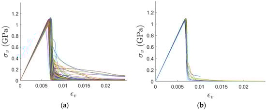
Figure 9.
Vertical stress vs. strain overlay for (a) 56 μm; (b) 140 μm.
A few trends can be observed. First, for both sizes, there are more variations in fracture (maximum and post-maximum stress) than there are in elastic response. Second, the variations in both elastic and fracture properties are more noticeable for the smaller SVEs in Figure 9a. Third, the captured response is a relatively brittle pre-maximum stress level. In reference [46], several brittleness indicators are defined based on the ratios of initiation (i.e., where the stress–strain response before the maximum stress significantly deviates from the linear response), maximum (where the stress is the maximum), and final (the first instance when the stress reaches zero) strains or energies. For example, in Figure 9, the ratio of strain at the initiation stage to that at the maximum stage is very close to one, reflecting the little softening response before the elastic branches reach the maximum stress level, and indicating a brittle failure response.
Figure 10a shows the probability distribution function (PDF) plots of for all relative SVE sizes. As can be seen, the variation in decreases as the SVE size increases. This is in agreement with the second observation above for the two relative SVE sizes of 56 and 140 μm. Interestingly, the mean and mode of are relatively unaffected as a function of SVE size. Another important vertical elastic material property is , the vertical normal component of the elasticity stiffness matrix. Due to Poisson effects, is not equal to . For brevity, we do not present the results for , but note that similar trends to are observed for The red dot corresponds to the experimental value reported in Table 1 from [38] and is provided as a reference point for other sample size results. The experimental sample, called RVE in this paper, is about six times larger than the largest SVE size of 140 μm. Thus, if we had more experimental images for this material, we would have expected the PDF of for this size to be a narrower bell-shaped curve than that of 140 μm, around the red dot.
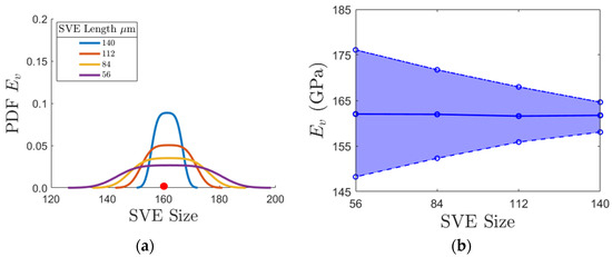
Figure 10.
Vertical results for : (a) PDF of for all SVE sizes. The red dot serves as a reference to the published value from [38]; (b) the size effect plot for .
Size effect relation of vertical stiffness is shown in Figure 10b. The minimum and maximum values of homogenized stiffness for the population of SVEs at any given size are shown by the dashed and dot-dashed lines. The mean value of the homogenized property is shown by the solid line inside this region. As implied by the PDFs in Figure 10a, we observe that the mean value of is quite stable among all SVE sizes. Moreover, there exists a relative difference of only 0.0027 across means values for each SVE size, highlighting that is not size-sensitive. In [26], a mean-based RVE size limit criterion is proposed, wherein the RVE size for a property is defined as the size at which the mean value of the given property is close enough to its terminal value (in the limit of infinite VE size). We observe that from this perspective, even the smallest relative SBE, 56 μm, can be considered a RVE size for whose mean value closely aligns with that of the published value in Table 1. The variations in gradually decrease from about 10% to 2.5% of the mean value as the SVE size increases. The decrease in variations is expected as in the limit of a SVE size equal to infinity, all VEs have the same response and the variation tends toward zero.
PDF and size effect plots of vertical strength, , are shown in Figure 11. The size effect plot in in Figure 11b shows a similar trend to that of vertical stiffness in Figure 10b, although the mean value is not as stable as across all SVE sizes, and the variations are higher for the smallest SVE sizes (15% for compared to 10% for for the SVE size 56 μm). This instability in the mean for is more evident in the PDFs of strengths (Figure 11a). This is expected as fracture properties are more sensitive to minute differences in the layout of the material at the microscale and in general, higher variations are experienced for fracture properties than they are for elastic ones [26]. Like in Figure 10a, the experimental value for the RVE (Figure 2a) is shown by the red dot in Figure 11a, for a comparison with the PDFs of the results of different SVE sizes.
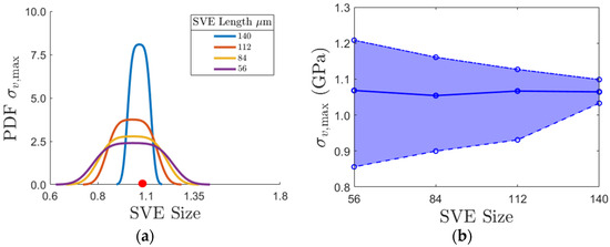
Figure 11.
Vertical results for : (a) PDF of for all SVE sizes. The red dot serves as a reference to the published value from [38]; (b) the size effect plot for .
3.2. Horizontal Direction
Figure 12 shows strain versus stress results in the horizontal direction for SVEs of sizes 56 and 140 μm, respectively. Compared to the corresponding results for vertical loading in Figure 10, there is less variation in the elastic modulus and delayed softening past the maximum stress for the horizontal loading results. We contribute these features to the topology of the melt pools in Figure 2a. The melt pool boundaries are more favorably opened when the loading is along the vertical direction compared to when it is in the horizontal direction. This is due to the fact that for horizontal loading, there are long stretches of material from left to right that carry the load and contain no melt pool lines. Accordingly, separation along the cohesive surfaces is not activated as much. The results show less variation and unloading past the maximum stress given that the response is mostly driven by the elastoplasticity of the bulk material.
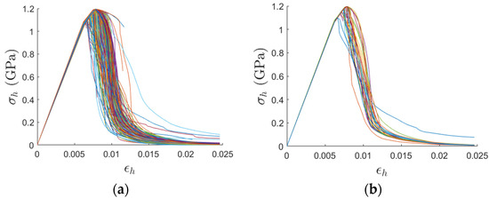
Figure 12.
Horizontal stress vs. strain overlay for (a) 56 μm; (b) 140 μm.
Figure 13 shows the PDF and size effect results for the horizontal stiffness. Referring to Figure 13b, stiffness for the horizontal load case is not as heavily affected by the varying SVE size as the vertical stiffness is in Figure 11b. Otherwise, both the vertical and horizontal stiffnesses show the same trends in the PDFs and size effects. That is, in both cases, the mean value stays relatively insensitive to the SVE size. The mean value for each SVE size also closely aligns with the publish value for in Table 1. This is reflected by the red dot corresponding to the experimental results in [38] for the RVE in Figure 2a.
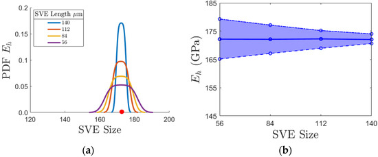
Figure 13.
Horizontal results for : (a) PDF of for all SVE sizes. The red dot serves as a reference to the published value from [38]; (b) the size effect plot of for all SVE sizes.
Figure 14 shows the results for horizontal strength Referring to the PDFs in Figure 14a, the mean value for varies more dramatically, close to tenfold more, compared to the elastic modulus . Again, the red dot corresponding to the experimental results in [38] is provided for comparison with computational results of different SVE sizes. Figure 14b illustrates the increase in both the mean and minimum homogenized value of as SVE size increased. The reason for the increase to at larger SVE sizes and the difference between horizontal and vertical elastic moduli is explained by referring to the geometry of the melt pools in Figure 2a and Figure 5. For large SVEs, there is a higher likelihood of having a whole block of bulk material that runs across the entire SVE. Such blocks prevent the failure of the SVE through debonding across cohesive surfaces, as none will run across the layer. These stiff layers dictate the overall stiffness in the horizontal direction; the 3D printed layers in this case act as parallel springs, wherein the highest stiffness (the continuous layers) dictates the overall stiffness. For small SVEs, there is more likelihood of having certain melt pool lines cut through a layer. Accordingly, the overall horizontal strength becomes lower for such small SVEs. In contrast, for all SVE sizes, the debonding in the vertical direction is easier and almost always possible, thus much less size sensitivity is observed in Figure 11 for . The decrease of variations for and is expected as both properties tend to their variation-based RVE size as the SVE size increases [12].
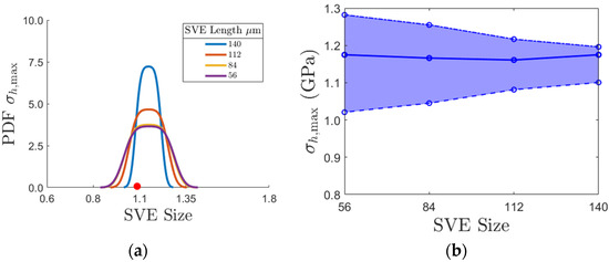
Figure 14.
Horizontal results for (a) PDF of for all SVE sizes. The red dot serves as a reference to the published value from [38]; (b) Size effect plot for .
4. Discussion
In this section, we summarize the results from the presented numerical results in the prior sections. First, we examine whether or not one can claim any of the four homogenized properties has reached its RVE size for 140 μm. In [26], we discussed mean-based, variation-based and boundary condition (BC)-based criteria to examine whether or not a homogenized properties has reached its RVE size limit. In the mean-based criterion, the RVE size is defined as the , such that for all SVEs larger than that, the relative variations in the mean value (e.g., the middle line in Figure 10b, Figure 11b, Figure 13b and Figure 14b) stay below a certain user-defined threshold, , across all larger SVE sizes. In the variation-based criterion, the RVE size corresponds to the size beyond with the coefficient of variation (COV) staying below the threshold, . The COV is defined as the ratio of the standard deviation to the mean value of the quantity. Often, the arbitrary threshold of = 0.01 is used for both criteria [22,25]. This variation-based criterion is the most common choice to determine the RVE size in the literature; see for example [25,47]. We refer the reader to [26] for a further discussion of these criteria and the BC-based criterion not used in this work.
In [26], we first obtain best fits to the means and COVs of a homogenized property versus before determining when the normalized mean and COV fall below for the definition of mean- and variation-based RVEs. In this work, we adopt a simpler approach given the lower variation in homogenized properties discussed in Section 3. For the mean-based criterion, we define the error in the mean values, e(μ), as the largest difference between the mean values of all sizes divided by the largest mean value. That is, it is a relative error among all the mean values of the given property. These values are reported in the first data row of Table 3. As evident, for all properties, e(μ) is below or very close to = 0.01. Thus, from this perspective, all homogenized properties can be claimed to have reached the mean-based RVE size below or around 140 μm.
Table 3.
Summary of values used to examine mean- and variation-based RVE sizes for all four homogenized properties.
The results for the variation-based criterion are shown in the second data line of Table 3. Herein, the COVs of the largest SVE size of 140 μm are provided. For elastic properties and vertical strength, the COVs are below = 0.01. Even for the homogenized strength, the COV of 0.023 is close to the often-used threshold of 0.01. Thus, even for the variation-based criterion, the properties are deemed to have reached their RVE size below or around 140 μm. This is an anticipated result, as [48] also obtained a similar finding pertaining to elastic properties.
Next, we examine the differences in the homogenized properties from two perspectives. First, for both criteria, elastic properties take smaller values, implying that they reach their RVE limit at a smaller size. This is consistent with our results in [26,41] for different two-phase composites. In [41], stress contours demonstrate that minute local variations in the microstructure result in highly varied levels of stress concentration and thus the strength value assigned to an SVE. In contrast, the elastic properties reflect the average response of the SVE (as opposed to the weakest point-type response for fracture properties) and are less sensitive to microstructural variations. This explains why the values for elastic properties are smaller in Table 3.
Second, we examine the difference between horizontal and vertical properties. From Table 3, we observe that that the homogenized not only has a more stable mean value (reflected in e(μ)), but also has smaller normalized variations (reflected in COV). Both aspects are also graphically evident when comparing Figure 10b and Figure 13b. This can be attributed to whole regions spanning the RVE horizontally, acting as rather deterministic parallel springs for the horizontal loading case. For fracture properties, while a lower variation is observed for compared to that for in Figure 11b and Figure 14b and in Table 3, one needs to refer to the actual strain–stress responses in Figure 9 and Figure 12 to have a clearer understanding of the differences of the two loading beyond just the maximum stress. From the strain–stress responses, we observe a lower variation in the elastic slope, , compared to that in (consistent with the COV values for 140 μm in Table 3). In contrast, it is now the horizontal direction that has a higher variation in response post-elastic regime.
5. Conclusions
The SVE-based homogenization approach can be used to derive elastic and fracture properties for SLM materials. The mean apparent values for vertical and horizontal QoIs bear a resemblance to the experimentally obtained values. Furthermore, increasing the SVE size reduces the variation in homogenized properties. The relative difference in mean values for was more than twice that for , indicating heightened sensitivity in the effect of SVE size on vertical stiffness. The behavior in the horizontal and vertical directions appears to exhibit inverse tendencies, with the vertical direction displaying heightened sensitivity in linear components while the horizontal direction demonstrates increased variability during fracture, indicating divergent behavior between the two directions. The difference in behavior between horizontal and vertical results can be attributed to the microstructure of the SLM material. The likelihood of a melt pool boundary perpendicular to the applied load is greater for the vertical load case than for the horizontal load case. The resulting over-stiffness phenomenon observed for the horizontal load case decreased for larger SVEs. As for fracture properties, we observe that they exhibit higher variations and less stable mean values when compared to those of elastic properties. In any case, for the SLM material considered, below or around the size of 140 μm, all elastic and fracture properties reached both the mean- and variation-based RVE size.
The results provide insights into how SLM materials’ elastic and fracture properties tend toward their macroscopic size-independent and homogeneous limit. While these RVE-based limits are suitable for many macroscopic problems, SVE-based homogenized properties are favorable for failure analysis as they maintain a sufficient level of material heterogeneity needed for such applications [26,41]. The heightened sensitivity of fracture properties to small variations in SLM materials bears significant implications for material design and structural integrity. A more comprehensive understanding of the brittleness and fracture behavior becomes critical since even minor variations in these properties can potentially lead to catastrophic brittle failures in real-world applications. We believe that these SVE-based elastic and fracture properties can be used for the stochastic failure analysis of materials as demonstrated in [30].
Some other extensions of this work are as follows. First, we only had one set of experimental results to compare with our computational results. To accurately validate the results, we should have several experimental strain–stress responses of the SLM material for each SVE size considered. Second, the temperature effects during manufacturing and ensuing residual stresses should be included in subsequent mechanical analysis. These residual stresses are obtained from the thermomechanical analysis of the printing process [49]. Some examples of such analysis for a single laser path, multiple parallel paths, and an entire SLM part are provided in [50,51], and [52], respectively. In future work, we aim to derive residual stresses resulting from simulating the manufacturing process and incorporating their effect on the nonlinear properties of the printed material, such as strength and fracture energy. Third, grain-level nonlinear material models such as crystal plasticity remove the restriction of crack propagation along melt pool boundaries and provide a more accurate overall representation of material failure. Fourth, SVE-based homogenization can be incorporated in the multiscale linear and nonlinear analysis of SVEs. The lower computational cost of such multiscale analyses (compared to that for DNS) makes this approach a suitable forward solver in design problems, for example in optimizing SLM printing parameters [50,53].
Author Contributions
Conceptualization, R.A., S.S., C.T.F. and K.L.; methodology, R.A. and S.S.; software, B.V., R.P.C., G.H., and R.A.; validation, R.P.C.; formal analysis, R.P.C.; investigation, R.P.C.; resources, C.T.F. and K.L.; data curation, R.P.C.; writing—original draft preparation, R.P.C., R.A. and B.V.; writing—review and editing, S.S., C.T.F. and K.L.; visualization, R.P.C. and B.V.; supervision, R.A., S.S., C.T.F. and K.L.; project administration, R.A., C.T.F. and K.L.; funding acquisition, R.A., C.T.F. and K.L. All authors have read and agreed to the published version of the manuscript.
Funding
This research was funded by Southeastern Advanced Machine Tools Network (SEAMTN), grant number SEAMTN-01-2022 with the federal Award Number HQ00052110069.
Data Availability Statement
The data presented in this study are available on request from the corresponding author. The data are not publicly available as the material and research are ongoing.
Acknowledgments
We acknowledge the support of SEAMTN project at the University of Tennessee Knoxville (UTK). We especially thank the support and leadership of the SEAMTN director Tony Schmitz and project manager Rhnea Reagan.
Conflicts of Interest
The authors declare that this study received funding from Southeastern Advanced Machine Tools Network (SEAMTN), grant number SEAMTN-01-2022 with the federal Award Number HQ00052110069. The funders had no role in the design of the study; in the collection, analyses, or interpretation of data; in the writing of the manuscript; or in the decision to publish the results.
References
- Carter, L.N.; Martin, C.; Withers, P.J.; Attallah, M.M. The influence of the laser scan strategy on grain structure and cracking behaviour in SLM powder-bed fabricated nickel superalloy. J. Alloys Compd. 2014, 615, 338–347. [Google Scholar] [CrossRef]
- Qiu, C.; Adkins, N.J.; Attallah, M.M. Microstructure and tensile properties of selectively laser-melted and of HIPed laser-melted Ti–6Al–4V. Mater. Sci. Eng. A 2013, 578, 230–239. [Google Scholar] [CrossRef]
- Zou, S.; Xiao, X.; Li, Z.; Liu, M.; Zhu, C.; Zhu, Z.; Xhen, C.; Zhu, F. Comprehensive investigation of residual stress in selective laser melting based on cohesive zone model. Mater. Today Commun. 2022, 31, 103283. [Google Scholar] [CrossRef]
- Choo, H.; Sham, K.-L.; Bohling, J.; Ngo, A.; Xiao, X.; Ren, Y.; Depond, P.J.; Matthews, M.J.; Garlea, E. Effect of laser power on defect, texture, and microstructure of a laser powder bed fusion processed 316 L stainless steel. Mater. Des. 2019, 164, 107534. [Google Scholar] [CrossRef]
- Andani, M.T.; Karamooz-Ravari, M.R.; Mirzaeifar, R.; Ni, J. Micromechanics modeling of metallic alloys 3D printed by selective laser melting. Mater. Des. 2018, 137, 204–213. [Google Scholar] [CrossRef]
- Andani, M.T.; Ghodrati, M.; Karamooz-Ravari, M.R.; Mirzaeifar, R.; Ni, J. Damage modeling of metallic alloys made by additive manufacturing. Mater. Sci. Eng. A 2019, 743, 656–664. [Google Scholar] [CrossRef]
- Shifeng, W.; Shuai, L.; Qingsong, W.; Yan, C.; Sheng, Z.; Yusheng, S. Effect of molten pool boundaries on the mechanical properties of selective laser melting parts. J. Mater. Process. Technol. 2014, 214, 2660–2667. [Google Scholar] [CrossRef]
- Riedlbauer, D.; Scharowsky, T.; Singer, R.F.; Steinmann, P.; Körner, C.; Mergheim, J. Macroscopic simulation and experimental measurement of melt pool characteristics in selective electron beam melting of Ti-6Al-4V. Int. J. Adv. Manuf. Technol. 2017, 88, 1309–1317. [Google Scholar] [CrossRef]
- Belotti, L.P.; Hoefnagels, J.; Geers, M.; van Dommelen, J. A modular framework to obtain representative microstructural cells of additively manufactured parts. J. Mater. Res. Technol. 2022, 21, 1072–1094. [Google Scholar] [CrossRef]
- Pilgar, C.M.; Fernandez, A.M.; Lucarini, S.; Segurado, J. Effect of printing direction and thickness on the mechanical behavior of SLM fabricated Hastelloy-X. Int. J. Plast. 2022, 153, 103250. [Google Scholar] [CrossRef]
- Cao, M.; Liu, Y.; Dunne, P. A crystal plasticity approach to understand fatigue response with respect to pores in additive manufactured aluminum alloys. Int. J. Fatigue 2022, 161, 106917. [Google Scholar] [CrossRef]
- Ji, L.; Wang, S.; Wang, C.; Zhang, Y. Effect of hatch space on morphology and tensile property of laser powder bed fusion of Ti6Al4V. Opt. Laser Technol. 2022, 150, 107929. [Google Scholar] [CrossRef]
- Hao, L.; Wang, W.; Zeng, J.; Song, M.; Chang, S.; Zhu, C. Effect of scanning speed and laser power on formability, microstructure, and quality of 316 L stainless steel prepared by selective laser melting. J. Mater. Res. Technol. 2023, 25, 3189–3199. [Google Scholar] [CrossRef]
- Li, E.; Zhang, Z.; Chang, C.; Li, L.Q. Numerical homogenization for incompressible materials using selective smoothed finite element method. Compos. Struct. 2015, 123, 216–232. [Google Scholar] [CrossRef]
- Zou, S.; Xiao, H.; Ye, F.; Li, Z.; Tang, W.; Zhu, F.; Chen, C.; Zhu, C. Numerical analysis of the effect of the scan strategy on the residual stress in the multi-laser selective laser melting. Results Phys. 2020, 16, 103005. [Google Scholar] [CrossRef]
- Hill, R. Elastic properties of reinforced solids: Some theoretical principles. J. Mech. Phys. Solids 1963, 11, 357–372. [Google Scholar] [CrossRef]
- Hill, R. On constitutive macro-variables for heterogeneous solids at finite strain. Proceedings of the Royal Society A: Mathematical. Phys. Eng. Sci. 1972, 326, 131–147. [Google Scholar]
- Mandel, J. Contribution th’eorique á l’étude de l’écrouissage et des lois de l’écoulement plastique. In Applied Mechanics; Springer: Berlin/Heidelberg, Germany, 1966; pp. 502–509. [Google Scholar]
- Ogden, R. On the overall moduli of non-linear elastic composite materials. J. Mech. Phys. Solids 1974, 22, 541–555. [Google Scholar] [CrossRef]
- Sab, K. On the homogenization and the simulation of random materials on the homogenization and the simulation of random materials. Eur. J. Mech. A-Solids 1992, 11, 585–607. [Google Scholar]
- Gitman, I.M.; Askes, H.; Sluys, L.J. Representative volume: Existence and size determination. Eng. Fract. Mech. 2007, 74, 2518–2534. [Google Scholar] [CrossRef]
- Pelissou, C.; Baccou, J.; Monerie, Y.; Perales, F. Determination of the size of the representative volume element for random quasi-brittle composites. Int. J. Solids Struct. 2009, 46, 2842–2855. [Google Scholar] [CrossRef]
- Ostoja-Starzewski, M. Random field models of heterogeneous materials. Int. J. Solids Struct. 1998, 35, 2429–2455. [Google Scholar] [CrossRef]
- Ostoja-Starzewski, M.; Du, X.; Khisaeva, Z.F.; Li, W. Comparisons of the size of the representative volume element in elastic, plastic, thermoelastic, and permeable random microstructures. Int. J. Multiscale Comput. Eng. 2007, 5, 73–82. [Google Scholar] [CrossRef]
- Kanit, T.; Forest, S.; Galliet, I.; Mounoury, V.; Jeulin, D. Determination of the size of the representative volume element for random composites: Statistical and numerical approach. Int. J. Solids Struct. 2003, 40, 3647–3679. [Google Scholar] [CrossRef]
- Abedi, R.; Garrard, J.; Acton, K.; Soghrati, S. Effect of boundary condition and statistical volume element size on inhomogeneity and anisotropy of apparent properties. Mech. Mater. 2022, 173, 104408. [Google Scholar] [CrossRef]
- Huyse, L.; Maes, M.A. Random field modeling of elastic properties using homogenization. J. Eng. Mech. 2001, 127, 27–36. [Google Scholar] [CrossRef]
- Segurado, J.; Llorca, J. Computational micromechanics of composites: The effect of particle spatial distribution. Mech. Mater. 2006, 38, 873–883. [Google Scholar] [CrossRef]
- Tregger, N.; Corr, D.; Graham-Brady, L.; Shah, S. Modeling the effect of mesoscale randomness on concrete fracture. Probabilistic Eng. Mech. 2006, 21, 217–225. [Google Scholar] [CrossRef]
- Bazant, Z.P.; Planas, J. Fracture and Size Effect in Concrete and Other Quasi-Brittle Materials; CRC Press: Rutledge, NY, USA, 1998; Volume 16. [Google Scholar]
- Genet, M.; Couegnat, G.; Tomsia, A.P.; Ritchie, R.O. Scaling strength distributions in quasi-brittle materials from micro- to macro-scales: A computational approach to modeling nature inspired structural ceramics. J. Mech. Phys. Solids 2014, 68, 93–106. [Google Scholar] [CrossRef]
- Strack, O.E.; Leavy, R.B.; Brannon, R.M. Aleatory uncertainty and scale effects in computational damage models for failure and fragmentation. Int. J. Numer. Methods Eng. 2015, 102, 468–495. [Google Scholar] [CrossRef]
- Dimas, L.S.; Giesa, T.; Buehler, M.J. Coupled continuum and discrete analysis of random heterogeneous materials: Elasticity and fracture. J. Mech. Phys. Solids 2014, 63, 481–490. [Google Scholar] [CrossRef]
- Baxter, S.C.; Graham, L.L. Characterization of random composites using moving-window technique. J. Eng. Mech. 2000, 126, 389–397. [Google Scholar] [CrossRef]
- Graham, L.L.; Baxter, S.C. Simulation of local material properties based on moving-window GMC. Probabilistic Eng. Mech. 2001, 16, 295–305. [Google Scholar] [CrossRef]
- Al-Ostaz, A.; Jasiuk, I. Crack initiation and propagation in materials with randomly distributed holes. Eng. Fract. Mech. 1997, 58, 395–420. [Google Scholar] [CrossRef]
- Kozicki, J.; Tejchman, J. Effect of aggregate structure on fracture process in concrete using 2D lattice model. Arch. Mech. 2007, 59, 365–384. [Google Scholar]
- Hanzl, P.; Zetek, M.; Bakša, T.; Kroupa, T. The Influence of Processing Parameters on the Mechanical Properties of SLM Parts. Procedia Eng. 2015, 100, 1405–1413. [Google Scholar] [CrossRef]
- Soghrati, S.; Nagarajan, A.; Liang, B. Conforming to interface structured adaptive mesh refinement: New technique for the automated modeling of materials with complex microstructures. Finite Elem. Anal. Des. 2017, 125, 24–40. [Google Scholar] [CrossRef]
- Soghrati, S.; Xiao, F.; Nagarajan, A. A conforming to interface structured adaptive mesh refinement technique for modeling fracture problems. Comput. Mech. 2017, 59, 667–684. [Google Scholar] [CrossRef]
- Bahmani, B.; Yang, M.; Nagarajan, A.; Clarke, P.L.; Soghrati, S.; Abedi, R. Automated homogenization-based fracture analysis: Effects of SVE size and boundary condition. Comput. Methods Appl. Mech. Eng. 2019, 345, 701–727. [Google Scholar] [CrossRef]
- Abaqus. Abaqus Analysis User’s Manual (V6.6); Washington University: St. Louis, MO, USA, 2006. [Google Scholar]
- Huet, C. Application of variational concepts to size effects in elastic heterogeneous bodies. J. Mech. Phys. Solids 1990, 38, 813–841. [Google Scholar] [CrossRef]
- Hazanov, S.; Huet, C. Order relationships for boundary conditions effect in heterogeneous bodies smaller than the representative volume. J. Mech. Phys. Solids 1994, 42, 1995–2011. [Google Scholar] [CrossRef]
- Hazanov, S.; Amieur, M. On overall properties of elastic heterogeneous bodies smaller than the representative volume. Int. J. Eng. Sci. 1995, 33, 1289–1301. [Google Scholar] [CrossRef]
- Ming, Y.; Abedi, R.; Garrard, J.; Soghrati, S. Effect of microstructural variations on the failure response of a nano-enhanced polymer: A homogenization-based statistical analysis. Comput. Mech. 2021, 67, 315–340. [Google Scholar]
- Liu, W.K.; Siad, L.; Tian, R.; Lee, S.; Lee, D.; Yin, X.; Chen, W.; Chan, S.; Olson, G.B.; Lindgen, L.E.; et al. Complexity science of multiscale materials via stochastic computations. Int. J. Numer. Methods Eng. 2009, 80, 932–978. [Google Scholar] [CrossRef]
- Jiang, Z.; Xu, P.; Liang, Y.; Liang, Y. Deformation effect of melt pool boundaries on the mechanical property anisotropy in the SLM AlSi10Mg. Mater. Today Commun. 2023, 36, 106879. [Google Scholar] [CrossRef]
- Luo, Z.; Zhao, Y. A survey of finite element analysis of temperature and thermal stress fields in powder bed fusion Additive Manufacturing. Addit. Manuf. 2018, 21, 318–332. [Google Scholar] [CrossRef]
- Letenneur, M.; Kreitcberg, A.; Brailovski, V. Optimization of laser powder bed fusion processing using a combination of melt pool modeling and design of experiment approaches: Density control. J. Manuf. Mater. Process. 2019, 3, 21. [Google Scholar] [CrossRef]
- Burkhardt, C.; Soldner, D.; Mergheim, J. A comparison of material models for the simulation of selective beam melting processes. Procedia CIRP 2020, 94, 52–57. [Google Scholar] [CrossRef]
- Luo, Z.; Zhao, Y. Numerical simulation of part-level temperature fields during selective laser melting of stainless steel 316 L. Int. J. Adv. Manuf. Technol. 2019, 104, 1615–1635. [Google Scholar] [CrossRef]
- Sun, Z.; Tan, X.; Tor, S.B.; Yeong, W.Y. Selective laser melting of stainless steel 316 L with low porosity and high build rates. Mater. Des. 2016, 104, 197–204. [Google Scholar] [CrossRef]
Disclaimer/Publisher’s Note: The statements, opinions and data contained in all publications are solely those of the individual author(s) and contributor(s) and not of MDPI and/or the editor(s). MDPI and/or the editor(s) disclaim responsibility for any injury to people or property resulting from any ideas, methods, instructions or products referred to in the content. |
© 2023 by the authors. Licensee MDPI, Basel, Switzerland. This article is an open access article distributed under the terms and conditions of the Creative Commons Attribution (CC BY) license (https://creativecommons.org/licenses/by/4.0/).