Identification of Hydrodynamic Coefficients of the SUBOFF Submarine Using the Bayesian Ridge Regression Model

Abstract

Maneuverability is one of the submarine’s most important features, and is closely related to hydrodynamic coefficients. The submarine standard motion equation is the most commonly used hydrodynamic mathematical model, estimating more than 100 hydrodynamic coefficients. This paper applies the Bayesian ridge regression model to identify a submarine’s hydrodynamic coefficients. Specifically, the proposed approach combines the URANS equation with a six-degree-of-freedom motion model and a body force propeller model, and uses overset grid technology to simulate the underwater six-degree-of-freedom navigation motion of the SUBOFF submarine. The submarine’s required hydrodynamic coefficients are obtained by collecting relevant velocity and angular velocity data and applying the Bayesian ridge regression model for data identification. Meanwhile, CFD simulation of the restraint model test for the SUBOFF submarine is conducted to obtain the related hydrodynamic coefficients. Through comparative experiments, we validate that the proposed Bayesian ridge regression model identification method is effective and reliable; most of the errors in the hydrodynamic coefficients were within 10%, with a maximum error of −43.26%, providing more comprehensive and timely hydrodynamic coefficients than traditional CFD restraint model tests. Furthermore, the hydrodynamic coefficient identification results were used to invert the submarine’s spatial motion, and we demonstrated that the resulting trajectory, velocity, and angular velocity curves all fit well.

1. Introduction

Accurate mathematical models are essential for research on submarine maneuvering and control. Currently, the dynamic mathematical model of submarines relies on the standard equations of submarine motion published by the United States Navy Ship Research and Development Center in 1967 [1]. However, these equations involve more than 100 hydrodynamic coefficients that must be estimated and obtained for accurate dynamic modeling.

Although free-running model tests are good for studying the maneuverability characteristics of submarines [2], they are costly and easily influenced by the experimental environment and measuring instruments. The restrained model tests of submarine models, including Planar Motion Mechanism (PMM) [3] and Rotation Arm (RA) [4], are widely used to obtain the hydrodynamic coefficients. RA can be used to obtain the cross coefficients related to angular velocities, but it is unable to determine acceleration derivatives and accurately measure position derivatives. Additionally, the experimental facilities for RA impose high costs. On the other hand, PMM is less expensive and can obtain more hydrodynamic coefficients by simulating the translational and rotational motions of the test model, thereby obtaining the six-degree-of-freedom hydrodynamic coefficients of the submarine hull, but the motion cannot be large in the PMM test, so the nonlinear coefficients are not reliable. Although most hydrodynamic coefficients can be obtained through these test methods, their high costs and long cycles remain practical problems.

With the development of computer technology, computational fluid dynamics (CFD) methods for simulating and calculating hydrodynamic coefficients have become more prevalent. For instance, Kim et al. [5] used CFD to simulate the PMM test of the KCS model and obtained partial hydrodynamic coefficients. Ji et al. [6] separated the linear and nonlinear components of the total resistance coefficient using CFD numerical methods, fitted the resistance coefficients for translational motion, and calculated the hydrodynamic coefficients for rotational motion using surface fitting. Wu et al. [7] combined the inertial and rotating reference frames, along with the added momentum source method, to simulate the RA test. By varying the angular velocity and drift angle, they obtained stability derivatives of yawing moment and yawing force that aligned well with the experimental results. Their study also explored the impact of the rotating arm radius. Gao et al. [8] extracted all hydrodynamic coefficients of the forced motion of a submarine hull by conducting only one test using CFD simulation.

Parameter identification methods are powerful technical means for establishing accurate system-dynamic mathematical models using experimental or numerical data. Many researchers have studied model identification and parameter estimation methods for autonomous underwater vehicles. For example, Abkowitz [9] first applied the Kalman filter for ship hydrodynamic parameter identification in the 1990s. Since then, numerous scholars have extended the research of [9], such as Ebrahimi et al. [10], who successfully determined the hydrodynamic coefficients of the NPS AUV II and ISIMI by employing velocity and displacement measurements in conjunction with the implementation of an extended Kalman filter (EKF) estimator. These hydrodynamic coefficients were then incorporated into the augmented state vector of a nonlinear model with six degrees of freedom. To enhance the accuracy and convergence speed of the algorithm, a suitable covariance matrix was selected based on the ARMA process model. Cardenas and de Barros [11] utilized a combination of an analytical and semi-empirical estimation (ASE) method that integrated the hydrodynamics and geometric characteristics of submarine vehicles. This approach was further enhanced by incorporating a parameter estimator based on the extended Kalman filter. To estimate the nominal hydrodynamic coefficients of the AUV, Sajedi and Bozorg [12] employed both the robust extended Kalman filter (REKF) and the extended H-infinity (EH∞) filter. Rasekh and Mahdi [13] employed a comprehensive approach combining the nonlinear hybrid extended Kalman filter (HEKF) observer, analytical and semi-empirical (ASE) formulas, as well as computational fluid dynamics (CFD) simulations. This combined method allowed for the estimation of all the hydrodynamic coefficients associated with a REMUS AUV. Scholars such as Mohammad et al. have also employed the Kalman filter and its improved algorithms to identify the hydrodynamic coefficients of underwater vehicles [14,15]. Additionally, Xiao [16] and Zhao [17] employed the maximum likelihood estimation algorithm to identify a simplified model of underwater vehicles and their hydrodynamic coefficients in different directions. Zhang et al. [18] and Mustafa et al. [19] utilized the least squares method to identify partial hydrodynamic coefficients of surface ships and underwater vehicles, respectively. Xue et al. [20] used the Bayesian method to identify the four-degree-of-freedom hydrodynamic coefficients of surface ships through simulated motion data. Additionally, some scholars have explored support vector machines [21,22], adaptive particle swarm optimization algorithms [23], and other algorithms to identify the hydrodynamic coefficients of surface and underwater vehicles.

This study introduces a new method for identifying the hydrodynamic coefficients of a six-degree-of-freedom underwater vehicle using the Bayesian ridge regression (BRR) model. The BRR algorithm was chosen due to its advantages of high data utilization, requiring fewer training samples, and avoiding overfitting [24]. Here, the BRR model is employed to solve the problem of extracting hydrodynamic coefficients for the complex motion of underwater vehicles with six degrees of freedom. Specifically, the CFD method is combined with the six-degree-of-freedom motion model, virtual propeller model, and overlapping grid technology to simulate the free navigation motion of a submarine model under specific rudder deflection. The motion and angular velocity data are collected, and then the model’s hydrodynamic coefficients are identified using the BRR model combined with the standard equations of submarine motion. Meanwhile, the CFD method simulates the restrained model test of the submarine model and obtains the partial hydrodynamic coefficients. Finally, the results of the two methods are compared, and the feasibility of the BRR model for identifying hydrodynamic coefficients is analyzed.

2. Mathematical Model

2.1. Submarine Motion Equation

Figure 1 illustrates the coordinate systems of a submarine, where the fixed coordinate system E-ξηζ is associated with the Earth and is the reference, and the moving coordinate system O-xyz moves along with the vehicle. Both coordinate systems are right-handed.

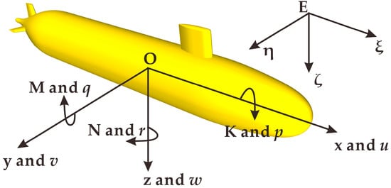
Figure 1. Coordinate systems of a submarine.

This study employs the standard submarine motion equations proposed by Gertler in 1967 [1]. Considering that the submarine undergoes low-speed and low-amplitude motion, the influence of the propeller load is neglected. Therefore, it is assumed that the propeller load remains constant during the maneuvering process of the submarine. The specific expression is as follows:

$$\left(\begin{array}{cccccc}m-X_{\dot{u}}& 0& 0& 0& m{z}_G& -m{y}_G\\ 0& m-Y_{\dot{v}}& 0& -m{z}_G-Y_{\dot{p}}& 0& m{x}_G-Y_{\dot{r}}\\ 0& 0& m-Z_{\dot{w}}& m{y}_G& -m{x}_G-Z_{\dot{q}}& 0\\ 0& -m{z}_G-K_{\dot{v}}& m{y}_G& I_x-K_{\dot{p}}& -I_{xy}& -I_{zx}-K_{\dot{r}}\\ m{z}_G& 0& -m{x}_G-M_{\dot{w}}& -I_{xy}& I_y-M_{\dot{q}}& -I_{yz}\\ -m{y}_G& m{x}_G-N_{\dot{v}}& 0& -I_{zx}-N_{\dot{p}}& -I_{yz}& I_z-N_{\dot{r}}\end{array}\right)\left(\begin{array}{c}\dot{u}\\ \dot{v}\\ \dot{w}\\ \dot{p}\\ \dot{q}\\ \dot{r}\end{array}\right)=\left(\begin{array}{c}{X}_1\\ Y_1\\ Z_1\\ K_1\\ M_1\\ N_1\end{array}\right)$$

(1)

where (x_G, y_G, z_G) denotes the coordinates of the center of gravity in the moving coordinate system; and u, v, w, p, q, and r represent the linear velocities along the x, y, and z axes, and the angular velocities around the x, y, and z axes, respectively. In Equation (1), the origin of the moving coordinate system does not coincide with the center of gravity. Additionally, X₁, Y_1, Z₁, K₁, M₁, and N₁ represent the axial force, lateral force, vertical force, rolling moment, pitching moment, and yawing moment acting on the submarine. The specific expressions for these terms are presented in Equations (2)–(7):

$$\begin{array}{cc}\hfill X_1& =\frac{1}{2}\rho L^4\left[X_{qq}^{\prime }{q}^2+X_{rr}^{\prime }{r}^2+X_{pp}^{\prime }{p}^2\right]+\frac{1}{2}\rho L^2\left[X_{uu}^{\prime }{u}^2+X_{vv}^{\prime }{v}^2+X_{ww}^{\prime }{w}^2\right]\hfill \\ & +\frac{1}{2}\rho L^3\left[X_{vr}^{\prime }vr+X_{wq}^{\prime }wq\right]+\frac{1}{2}\rho L^2{u}^2\left[X_{{\delta }_r{\delta }_r}^{\prime }{\delta }_r{}^2+X_{{\delta }_b{\delta }_b}^{\prime }{\delta }_b{}^2+X_{{\delta }_s{\delta }_s}^{\prime }{\delta }_s{}^2\right]\hfill \\ & -m\left[vr+wq-x_G(q^2+r^2)+y_{G}pq+z_{G}pr\right]-(P-B)\sin \theta +F_p\hfill \end{array}$$

(2)

$$\begin{array}{ll}{Y}_1& =\frac{1}{2}\rho L^4\left(Y_{p|p|}^{\prime }p|p|+Y_{pq}^{\prime }pq+Y_{qr}^{\prime }qr\right)+\frac{1}{2}\rho L^3\left(Y_{vq}^{\prime }vq+Y_{wp}^{\prime }wp+Y_{wr}^{\prime }wr\right)\\ & +\frac{1}{2}\rho L^2\left[Y_{vw}^{\prime }vw+Y_{{\delta }_r}^{\prime }{u}^2{\delta }_r\right]+\frac{1}{2}\rho L^2\left[Y_0^{\prime }{u}^2+Y_v^{\prime }uv+Y_{|v|v}^{\prime }v\left|{(v^2+w^2)}^{1/2}\right|\right]\\ & +\frac{1}{2}\rho L^3\left(Y_r^{\prime }ur+Y_{|r|{\delta }_r}^{\prime }u|r|{\delta }_r+Y_p^{\prime }up+Y_{v|r|}^{\prime }\frac{v}{|v|}\left|{(v^2+w^2)}^{1/2}\right||r|\right)\\ & -m\left[ur-wp+x_{G}pq-y_G(p^2+r^2)+z_{G}qr\right]+(P-B)\cos \theta \sin \phi \end{array}$$

(3)

$$\begin{array}{ll}{Z}_1& =\frac{1}{2}\rho L^4\left[Z_{pp}^{\prime }pp+Z_{rr}^{\prime }rr+Z_{rp}^{\prime }rp\right]+\frac{1}{2}\rho L^2\left[Z_{vv}^{\prime }vv+Z_{{\delta }_S}^{\prime }{u}^2{\delta }_S+Z_{{\delta }_b}^{\prime }{u}^2{\delta }_b\right]\\ & +\frac{1}{2}\rho L^3\left[Z_{vr}^{\prime }vr+Z_{vp}^{\prime }vp\right]+\frac{1}{2}\rho L^3\left[Z_q^{\prime }uq+Z_{\left|q\right|{\delta }_S}^{\prime }u\left|q\right|{\delta }_S+Z_{w\left|q\right|}^{\prime }u\frac{w}{\left|w\right|}\left|{(v^2+w^2)}^{1/2}\right|\left|q\right|\right]\\ & +\frac{1}{2}\rho L^2\left[Z_0^{\prime }{u}^2+Z_w^{\prime }uw+Z_{w\left|w\right|}^{\prime }w\left|{(v^2+w^2)}^{1/2}\right|+Z_{\left|w\right|}^{\prime }u\left|w\right|+Z_{ww}^{\prime }w{(v^2+w^2)}^{1/2}\right]\\ & -m\left[vp-uq+x_{G}rp+y_{G}rq-z_G(p^2+q^2)\right]+(P-B)\cos \theta \cos \phi \end{array}$$

(4)

$$\begin{array}{ll}{K}_1& =\frac{1}{2}\rho L^5\left[K_{qr}^{\prime }qr+K_{pq}^{\prime }pq+K_{p|p|}^{\prime }p|p|\right]\\ & +\frac{1}{2}\rho L^4\left[K_p^{\prime }up+K_r^{\prime }ur+K_{vq}^{\prime }vq+K_{wp}^{\prime }wp+K_{wr}^{\prime }wr\right]\\ & +\frac{1}{2}\rho L^3\left[K_0^{\prime }{u}^2+K_v^{\prime }uv+K_{{\delta }_r}^{\prime }{u}^2{\delta }_r+K_{v|v|}^{\prime }v\sqrt{v^2+w^2}+K_{vw}^{\prime }vw\right]\\ & -\left(I_{zz}-I_{yy}\right)qr+pq{I}_{zx}-\left(r^2-q^2\right)I_{yz}-I_{xy}pr-m\left[y_G(vp-uq)-z_G(ur-wp)\right]\\ & +\left(y_{G}P-y_{B}B\right)\cos \theta \cos \phi -\left(z_{G}P-z_{B}B\right)\cos \theta \sin \phi \end{array}$$

(5)

$$\begin{array}{ll}{M}_1& =\frac{1}{2}\rho L^5\left[M_{pp}^{\prime }pp+M_{rr}^{\prime }rr+M_{rp}^{\prime }rp+M_{q|q|}^{\prime }q\left|q\right|\right]+\frac{1}{2}\rho L^3\left[M_{vv}^{\prime }vv+M_{{\delta }_s}^{\prime }{u}^2{\delta }_s+M_{{\delta }_b}^{\prime }{u}^2{\delta }_b\right]\\ & +\frac{1}{2}\rho L^4\left[M_{vr}^{\prime }vr+M_{vp}^{\prime }vp+M_q^{\prime }uq+M_{\left|q\right|{\delta }_s}^{\prime }u\left|q\right|{\delta }_s+M_{\left|w\right|q}^{\prime }q\left|{\left(v^2+w^2\right)}^{1/2}\right|\right]\\ & +\frac{1}{2}\rho L^3\left[M_0^{\prime }{u}^2+M_w^{\prime }uw+M_{w|w|}^{\prime }w\left|{\left(v^2+w^2\right)}^{1/2}\right|+M_{|w|}^{\prime }u|w|+M_{ww}^{\prime }w\left|{\left(v^2+w^2\right)}^{1/2}\right|\right]\\ & -\left(I_{xx}-I_{zz}\right)rp+I_{xy}qr-\left(p^2-r^2\right)I_{zx}-I_{yz}qp-m\left[z_G(wq-vr)-x_G(vp-uq)\right]\\ & -\left(x_{G}P-x_{B}B\right)\cos \theta \cos \phi -\left(z_{G}P-z_{B}B\right)\sin \theta \end{array}$$

(6)

$$\begin{array}{ll}{N}_1& =\frac{1}{2}\rho L^5\left[N_{pq}^{\prime }pq+N_{qr}^{\prime }qr+N_{r|r|}^{\prime }r|r|\right]+\frac{1}{2}\rho L^4\left[N_{wr}^{\prime }wr+N_{wp}^{\prime }wp+N_{wq}^{\prime }vq\right]\\ & +\frac{1}{2}\rho L^4\left[N_p^{\prime }up+N_r^{\prime }ur++N_{\left|r\right|{\delta }_r}^{\prime }u\left|r\right|{\delta }_r+N_{\left|v\right|r}^{\prime }r\left|{\left(v^2+w^2\right)}^{1/2}\right|\right]\\ & +\frac{1}{2}\rho L^3\left[N_0^{\prime }{u}^2+N_v^{\prime }uv+N_{|v|v}^{\prime }v{\left(v^2+w^2\right)}^{1/2}+N_{vw}^{\prime }vw+N_{{\delta }_r}^{\prime }{u}^2{\delta }_r\right]\\ & -\left(I_{yy}-I_{xx}\right)pq+I_{yz}rp-\left(q^2-p^2\right)I_{xy}-I_{zx}rq-m\left[x_G(wp+ur)-y_G(vr+wq)\right]\\ & +\left(x_{G}P-x_{B}B\right)\cos \theta \cos \phi +\left(y_{G}P-y_{B}B\right)\sin \theta \end{array}$$

(7)

This work considers a simplified propeller model for the propulsion system, with negligible consideration given to the effects of load variations during maneuvering. The thrust force F_p is calculated using the following equation:

$$F_p=\rho n^2{D}_p^4{K}_T(1-t_p)$$

(8)

where ρ represents the fluid density, n denotes the propeller rotational speed, D_p corresponds to the propeller diameter, K_T represents the thrust coefficient, and t_p is the thrust deduction factor.

2.2. Bayesian Ridge Regression Model

The Bayesian ridge regression model is a linear regression model, and its general expression has the following form:

$$Y={\omega }^{T}X+\epsilon$$

(9)

where ω is the estimated random vector with a dimension of d; X = {x_i} and Y = {y_i} represent the system input and output random variables, i = 1, 2, 3, …; n denotes the sample size; and ε is the random noise that follows a Gaussian distribution with a mean of 0 and variance β.

The prior distribution assumption for parameter ω follows a Gaussian distribution:

$$P(\omega )=N(0,{\lambda }^{-1}I)$$

(10)

where I is the d × d identity matrix, λ is a hyperparameter that controls the prior distribution density, and λ⁻¹I represents the variance of the corresponding Gaussian distribution. We assume that the conditional probability of the output variable Y also follows a Gaussian distribution, which leads to the likelihood function of ω:

$$p(Y\mid \omega ,X)=N(Y\mid {\omega }^{T}x,{\sigma }^2)$$

(11)

where σ² is the corresponding variance.

From Equation (11), the posterior distribution of ω can be computed using the Bayesian theorem, expressed as follows:

$$p\left(\omega |x,Y\right)\propto p\left(Y|x,\omega \right)p\left(\omega \right)$$

(12)

Based on the likelihood function and prior distribution, further derivation leads to the following outcome:

$$p(\omega |x,Y)\propto \exp (-\frac{1}{2{\sigma }^2}{\displaystyle \sum _{i=1}^n{(y_i-{\omega }^T{x}_i-{\epsilon }_i)}^2})\exp (-\frac{\lambda }{2}{\omega }^T\omega )$$

(13)

The logarithmic form of this expression is as follows:

$$\ln p(\omega |x,y)\propto -\frac{1}{2{\sigma }^2}{\displaystyle \sum _{i=1}^n{(y_i-{\omega }^T{x}_i-{\epsilon }_i)}^2}-\frac{\lambda }{2}{\omega }^T\omega +const$$

(14)

where const is a constant unrelated to ω. According to the Bayesian statistical principles, it is evident that the posterior distribution of ω also follows a Gaussian distribution. This distribution is utilized for purposes involving the prediction and estimation of uncertainty.

The optimal parameters ω_MAP for Equation (14) are obtained by finding the extremum point. The resulting expression for ω_MAP is as follows:

$${\omega }_{MAP}={(\lambda I+\frac{1}{{\sigma }^2}{\displaystyle \sum _{i=1}^n{x}_i}{x}_i^T)}^{-1}\frac{1}{{\sigma }^2}{\displaystyle \sum _{i=1}^n{x}_i}{y}_i$$

(15)

where the matrix ${(\lambda I+\frac{1}{{\sigma }^2}{\displaystyle \sum _{i=1}^n{x}_i}{x}_i^T)}^{-1}$ is a d × d matrix. The mean square deviation σ and the parameter λ satisfy a gamma distribution:

$$\sigma ~Ga({\alpha }_1,{\alpha }_2)$$

(16)

$$\lambda ~Ga({\beta }_1,{\beta }_2)$$

(17)

In fitting the model, the joint estimation of parameters ω, σ, and λ is typically regulated using the Maximum A Posteriori (MAP) estimation method. Specifically, while solving the ω_MAP, the noise variance σ is regarded as an unknown parameter, and the optimal estimates for ω_MAP, σ, and λ are obtained by maximizing the posterior distribution [24,25].

In this study’s identification process, the standard equations of submarine motion are appropriately modified. Specifically, in Equation (1), the left-hand side represents the product of the mass matrix M and the acceleration matrix A, while the right-hand side represents the external forces F acting on the submarine, which can be abbreviated as:

$$M\cdot A=F$$

(18)

Then, the Euler method is used to discretize Equation (18), providing the following expression:

$$F=M\cdot \frac{V_{i+1}-V_i}{\Delta t}$$

(19)

where V = [u, v, w, p, q, r]^T, Δt represents the discrete time step, and i denotes the sampling time step, i = 0, 1, 2, …. By utilizing Equations (2) and (19), F can be obtained by solving for the force matrix using M and V. Consequently, each component of matrix F can be expressed linearly. Notably, the force in the x-axis direction, denoted as X₁, is expressed as follows:

$$X_1=X_{hy}\cdot x(i)-m\left[vr+wq-x_G\left(q^2+r^2\right)+y_{G}pq+z_{G}pr\right]-(P-B)\sin \theta +F_p$$

(20)

where the hydrodynamic derivatives and speed state variables in Equation (11) are as follows:

$$\begin{gathered} X_{hy}=\left[X_{qq}^{\prime },X_{rr}^{\prime },X_{rp}^{\prime },X_{vr}^{\prime },X_{wq}^{\prime },X_{uu}^{\prime },X_{vv}^{\prime },X_{ww}^{\prime },X_{{\delta }_r{\delta }_r}^{\prime },X_{{\delta }_b{\delta }_b}^{\prime },X_{{\delta }_s{\delta }_s}^{\prime }\right] \\ x(i)={\left[q_{(i)}{}^2,r_{(i)}{}^2,p_{(i)}{}^2,v_{(i)}{r}_{(i)},w_{(i)}{q}_{(i)},u_{(i)}{}^2,v_{(i)}{}^2,w_{(i)}{}^2,{u_{(i)}}^2{\delta }_{r_{(i)}}^2,{u_{(i)}}^2{\delta }_{b_{(i)}}^2,{u_{(i)}}^2{\delta }_{s_{(i)}}^2\right]}^T \end{gathered}$$

where X_hy represents the hydrodynamic coefficient in the x-direction that must be identified, and x(i) denotes the independent variable parameters at the time i. Similarly, the linear expressions for the remaining five force components in different directions can be derived, but these will not be elaborated upon in this discussion.

The hydrodynamic coefficient vector X_hy is the parameter ω in the Bayesian ridge regression model, with the data samples x(i) at a specific moment represented by x_i.

3. Model and CFD Methods

3.1. Model

The target model was a half-scale SUBOFF model [26], which is a standard DARPA design with publicly available geometric details. Figure 2 depicts the entire model, with the related coordinate system illustrated in Figure 1. The model scale ratio was 1:2, with a length of L = 2.178 m. Table 1 reports the remaining model parameters.

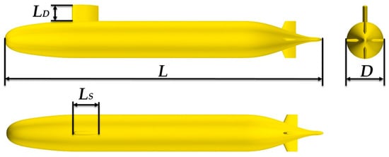
Figure 2. SUBOFF geometry.

Table 1. Main dimensional parameters for the SUBOFF model.

Parameter	Symbol	Unit	Value
Total length	L	m	2.178
Diameter	D	m	0.254
Sail length	LS	m	0.184
Sail height	LD	m	0.112
Mass of model	ms	kg	88.02
Center of mass	(xg, yg, zg)	m	(1.005, 0.0, −0.003)
Center of buoyancy	(xb, yb, zb)	m	(1.005, 0.0, 0.001)
Moment of inertia	(Ixx, Iyy, Izz)	kg·m2	(0.88, 25.43, 25.43)

3.2. CFD Methods

Numerical simulation was conducted using the commercial CFD software, STAR-CCM+ 13.02, which employs the incompressible unsteady Reynolds-averaged Navier–Stokes (RANS) equations in combination with the k-ω shear stress transport (SST) turbulence model. The selection of the k-ω SST turbulence model was based on its effective prediction capability and reasonable computational cost. The simulation strategy was guided using the studies conducted by Jak [27], and Dantas [28] as references to inform the design process, which is represented in a two-equation format:

$$\left\{\begin{array}{c}\frac{\partial (\rho k)}{\partial t}+\frac{\partial \left(\rho u_{j}k\right)}{\partial x_j}=P-{\beta }^{*}\rho \omega k+\frac{\partial }{\partial x_j}\left[\left(\mu +{\sigma }_k{\mu }_{\mathrm{t}}\right)\frac{\partial k}{\partial x_j}\right]\\ \frac{\partial (\rho \omega )}{\partial t}+\frac{\partial \left(\rho u_j\omega \right)}{\partial x_j}=\frac{\rho \gamma }{{\mu }_{\mathrm{t}}}P-{\beta }^{*}\rho {\omega }^2+\frac{\partial }{\partial x_j}\left[\left(\mu +{\sigma }_{\omega }{\mu }_{\mathrm{t}}\right)\frac{\partial \omega }{\partial x_j}\right]+2\left(1-F_1\right)\frac{\rho {\sigma }_{\omega 2}}{\omega }\cdot \frac{\partial k}{\partial x_j}\cdot \frac{\partial \omega }{\partial x_j}\end{array}\right.$$

(21)

where ρ represents density, μ_j denotes velocity vector, x_j indicates position vector, and k and ω represent turbulent kinetic energy and turbulence dissipation rate, respectively. The coefficients μ and μ_t correspond to laminar and turbulent viscosity coefficients. The form of the production term P and function F₁, as well as the values of coefficients β*, γ, σ_k, and σ_ω2, can be inferred from the relevant literature for the SST model [29].

In order to validate the accuracy of the numerical computation method and facilitate comparison with experimental data, the SUBOFF model was simulated at a scale ratio of 1:1. This corresponds to a model length of 4.356 m and an incoming flow velocity of 5.144 m/s. The drag force values from the towing experiment were calculated for reference [30]. This computational grid is presented in Figure 3.

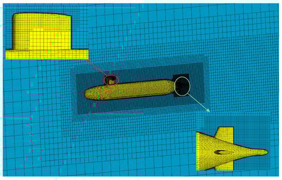
Figure 3. The computational region grid for resistance.

To ensure the convergence of the computational grid, the mesh was encrypted according to the fineness ratio in the ITTC recommendation rules. Specifically, the grid was encrypted in all three directions using r_G = $\sqrt{2}$; the other parameters were unchanged [31]. Table 2 reports three sets of grids with varying refinement levels, including the corresponding drag values obtained from towing experiments.

Table 2. Comparison between CFD methods and experimental value for the SUBOFF model (L = 4.356).

Method	Grid Level	Cells (Millions)	Drag Force (N)	Relative Error (%)
Experiment	-	-	283.8	-
CFD	Coarse	2.96	299.87	5.66%
	Medium	7.25	291.76	2.81%
	Fine	16.78	290.57	2.39%

Symbol Δ represents the difference in resistance between two types of grids:

Δ₁ = R_medium − R_fine

(22)

Δ₂ = R_coarse − R_medium

(23)

The changes in Δ were used to define the convergence ratio R_ratio:

R_ratio = Δ₁/Δ₂

(24)

The computed convergence ratio, R_ratio = 0.128, falls within the 0 < R_ratio < 1 range. Therefore, the three sets of grids exhibit monotonic convergence, and the drag force calculated for the medium grid resulted in an error of 2.81% when compared to the experimental data. This error falls below the 5% threshold, indicating a satisfactory level of accuracy. Considering all factors, using the medium grid for further investigations on the six-degrees-of-freedom motion of the SUBOFF model and the simulation of the constrained model experiment is recommended.

3.3. Spatial Motion Simulation

The CFD method was employed to simulate the spatial motion of the SUBOFF model and thus identify its hydrodynamic coefficients. In order to fully activate the model’s motion characteristics, the CFD numerical motion was conducted under some specified operating conditions. Once the model speed is stabilized, the horizontal and vertical rudders continuously steer in a sinusoidal pattern, thereby obtaining the simulated trajectory of the model’s spatial motion, which theoretically allows for the identification of all hydrodynamic coefficients of the SUBOFF model.

It should be noted that when simulating the model’s six-degrees-of-freedom motion, while the propeller propels the hull’s motion, the rotation of the horizontal and vertical rudders controls the direction of the hull. This is a complex motion system, and at the same time, the propeller, rudder, and vertical fin must move together with the hull. The overset grid technology can independently generate grids for different regions and flexibly handle the relative motion of multiple objects. Therefore, in the simulation process, the rotation motion of the horizontal and vertical rudders was handled using overset grids. In contrast, the submarine’s motion followed a six-degrees-of-freedom motion model, and the propeller motion was simplified using a body force model. This strategy has been validated in [32].

3.3.1. Grid

Figure 4 illustrates the hull’s computational region and the rudder’s overset grid region. In Figure 4a, the computational region of the hull is represented, where the rear boundary is set as a fluid pressure outlet located L distance away from the hull. The remaining boundary surfaces are all set as velocity inlets. The front boundary surface of the hull is also located at a distance of L from the hull, while the side surfaces are positioned at 0.5 L away from the hull, and the upper and lower boundary surfaces are at a distance of L from the hull. To ensure the movement of the overset grid, there is a 5 mm gap between the rudder and the hull. Figure 4b depicts the computational region of the rudder, with its boundaries defined as the Overset Interface.

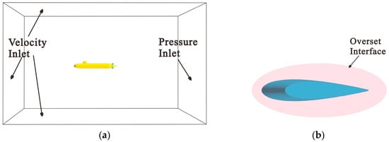
Figure 4. The computational regions. (a) Hull region; (b) rudder region.

Figure 5 illustrates the computational region grid. The hull and rudder region use a trimmer mesh, and the hull boundary layer comprises 5 layers with a target y+ value of approximately 1. The background grid in the rotating region of the rudder should be made as consistent as possible with the rudder region grid to ensure the interpolation accuracy and quality of the overset grids. Additionally, the propeller wake region is locally encrypted. Figure 5b displays the overset grid of the rudder region.

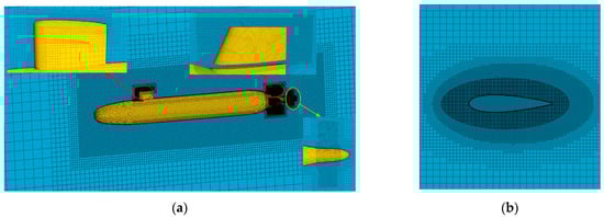
Figure 5. The region grids. (a) Hull region grid; (b) rudder region grid.

3.3.2. Body Force Propeller Model

The weighted integration of the flow velocity onto the propeller’s inflow plane provides the propeller’s inflow velocity, which is substituted into the propeller’s known hydrodynamic curve to estimate the thrust and torque. Subsequently, by adding source terms, an equivalent force and moment are exerted on the fluid within the specified volume force field. This method is referred to as the body force model [33]. Compared to conducting actual propeller calculations, this method has a higher computational efficiency. Therefore, the propeller was replaced by a virtual propeller based on the volume force model. This virtual propeller adopts the DTMB 4382 propeller parameters, which are reported in Table 3. Additionally, Figure 6 depicts the virtual propeller’s location within the submarine, the inflow plane diameter of the blade disk (D_i = 1.1D_P), and the offset of the inflow plane (d_s = 0.1D_P).

Table 3. Main parameters for DTMB4382.

Parameter	Symbol	Value
Blades	-	5
Diameter	DP	0.15
Hub-to-diameter ratio	d/DP	0.2
Disk aspect ratio	Ae/A0	0.725

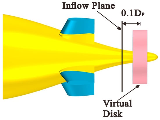
Figure 6. Relative position of the virtual propeller on the model.

Figure 7 illustrates the open-water performance curve. In order to obtain the same performance as the propeller, its characteristics should be incorporated into the volume force model, where the volume force depends on the thrust coefficient k_t and torque coefficient k_q. These coefficients are obtained from open-water experiments and are related to the advance ratio J:

$$J=V/(n{D}_p)$$

(25)

where n represents the rotational speed of the propeller, D_p is the propeller’s diameter, and V is the fluid velocity at the propeller location.

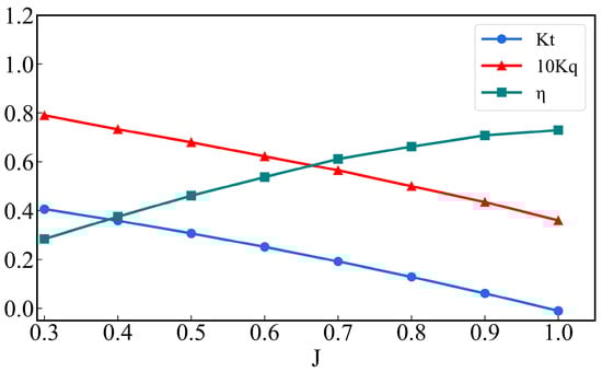
Figure 7. Open-water performance curve of propeller DTMB 4382.

3.3.3. Spatial Motion Result

The numerical simulations regarding the six-degree-of-freedom spatial motion have a time interval of Δ_t = 0.01 s, and the total duration is t = 200 s. To fully activate the SUBOFF model’s motion characteristics, the vessel performs CFD six-degree-of-freedom numerical navigation motion under specified operating conditions, i.e., the propeller rotates at n = 15 rad/s, while the horizontal rudder δ_s and the vertical rudder δ_r move in a sinusoidal pattern. Considering that the submarine standard equations are applicable for low-amplitude motion, the amplitude of the rudder angle was determined as 10 degrees, and the motion law of the rudder angle was given by δ_s (δ_r) = 10 sin(2π/30·t). The horizontal and vertical rudders have a motion period of 30 s. It took 126.4 h to compute it in the server utilizing three blades, with each blade having 128 GB of memory and 20 cores.

During the simulation of SUBOFF spatial motion, the collected velocity and angular velocity data were used to identify the hydrodynamic coefficients. Figure 8 depicts the model’s temporal curves for the velocity and angular velocity in different directions in the body coordinate system. Figure 9 presents an illustrative diagram of the motion trajectory of the SUBOFF model.

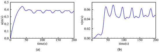
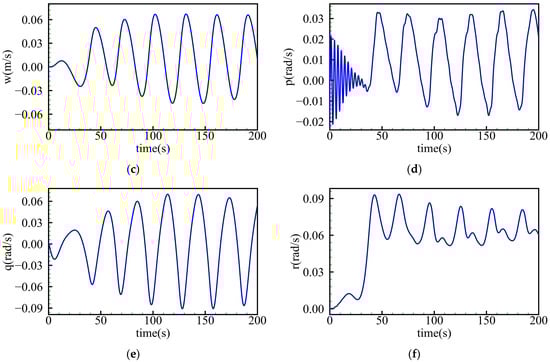
Figure 8. Time history curves of the SUBOFF model’s velocity and angular velocity. (a) X direction velocity u; (b) Y direction velocity v; (c) Z direction velocity w; (d) roll rate p; (e) pitch rate q; (f) yaw rate r.

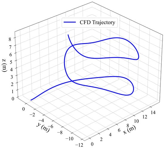
Figure 9. Spatial motion trajectory obtained from the virtual experiment.

Figure 10 presents a schematic diagram of the submarine’s vortex structures at different times. The wake region of the propeller is represented by a circular shape, which distinguishes it from the physical model and the discretized propeller vortex structure. Additionally, this figure illustrates horseshoe vortices caused by the hull, tip vortices, and hub vortices at different time points.

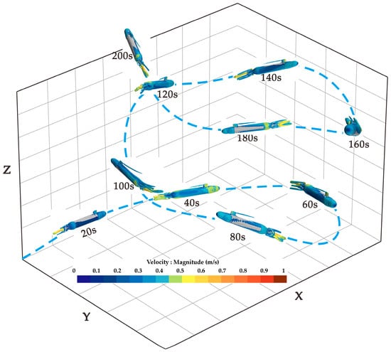
Figure 10. Vortex structures at different time points.

3.4. Simulated Restraint Model Test

A series of restraint model tests using CFD were conducted to compare the identification results under the same numerical calculation conditions. These tests included the oblique towing test, pure sway, pure yaw on the horizontal plane, and oblique towing test, pure pitch, and pure heave on the vertical plane. The mesh settings for each test condition are described in Section 3.2. Since the testing methodology for the vertical plane was consistent with that of the horizontal plane, the following paragraphs will discuss only the details of the vertical plane tests. The inflow velocity for all test conditions was set to 0.5 m/s.

3.4.1. Oblique Towing Tests on the Vertical Plane

The oblique towing tests measure the dimensionless position derivatives of the SUBOFF model. These tests vary the angle of attack (α) of the vessel within a range of −12° to 12°, with 2° intervals. The magnitude of the vertical force (Z) and the pitching moment (M) are measured under a constant flow velocity, as depicted in Figure 11.

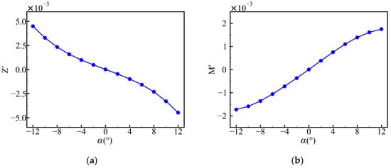
Figure 11. Oblique towing test results. (a) Angle of attack (α) against vertical force (Z); (b) angle of attack (α) against pitching moment (M).

3.4.2. Pure Heaving

The pure heaving motion of a submarine refers to the motion along its centerline on the vertical plane being uniform while simultaneously having a vertical displacement. The submarine’s heading remains unchanged and undergoes a sinusoidal motion with zero pitch angle. Figure 12 illustrates the concept of pure heaving motion.

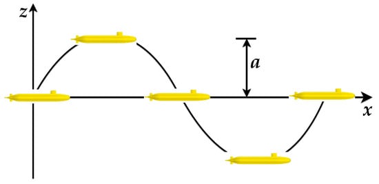
Figure 12. Model trajectory during the pure heaving test.

The expression for simulating pure heaving motion is as follows:

$$\left\{\begin{array}{l}\zeta =a\sin \omega t\hfill \\ \theta =\dot{\theta }=0\hfill \\ w=\dot{\zeta }=a\omega \cos \omega t\hfill \\ \dot{w}=-a{\omega }^2\sin \omega t\hfill \end{array}\right.$$

(26)

where ζ represents the vertical displacement of the submarine at any given moment, a is the amplitude of the motion, ω is the circular frequency of the motion, θ is the pitch angle, and $\dot{\theta }$ is the angular velocity. Additionally, w and $\dot{w}$ represent the vertical velocity and acceleration of the submarine.

The submarine model has a motion with a frequency of f = 0.2 Hz and an amplitude of a = 0.15 m. The simulation calculated data for 6 complete cycles and focused on the stable data from the 2nd to the 3rd cycle. The vertical force (Z) and the pitching moment (M) acting on the underwater body were monitored, with Figure 13 presenting the non-dimensional time history curves for Z and M in pure heaving motion.

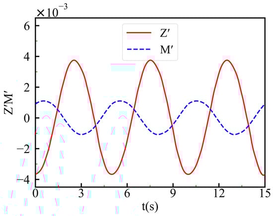
Figure 13. Curves for the vertical force (Z) and pitching moment (M) during pure heaving motion.

3.4.3. Pure Pitch

Pure pitch in a submarine refers to the combination of uniform motion along the centerline and a variation in pitch angle. This bow angle ensures that the submarine’s trajectory is always tangent to the body coordinate system’s vertical axis (z-axis). Figure 14 illustrates the concept of pure pitch.

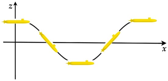
Figure 14. Trajectory of the model during the pure pitch test.

The simulated pure pitch motion is expressed as follows:

$$\left\{\begin{array}{l}\theta ={\theta }_0\sin \omega t\hfill \\ q=\dot{\theta }={\theta }_0\omega \cos \omega t\hfill \\ \dot{q}=-{\theta }_0{\omega }^2\sin \omega t\hfill \\ w=\dot{w}=0\hfill \end{array}\right.$$

(27)

where ${\theta }_0$ is the amplitude of the pitch motion, q is the angular velocity of the pitch angle, and $\dot{q}$ is the angular acceleration of the pitch angle.

In this trial, the submarine model has a motion with a frequency of f = 0.2 Hz. The simulation calculated data for 6 complete cycles and focused on the stable data from the 2nd to the 3rd cycle. The vertical force (Z) and the pitching moment (M) acting on the underwater body were monitored, with Figure 15 presenting the non-dimensional time history curves of Z and M in pure pitch motion.

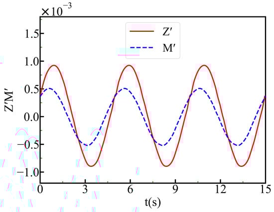
Figure 15. The non-dimensional time history curves for Z and M in pure pitch motion.

4. Results and Discussion

4.1. Results of Hydrodynamic Coefficient Identification

When identifying the hydrodynamic coefficients, the coefficient of determination R² is commonly used to evaluate the goodness of fit. The expression for R² is:

$$R^2=(1-\frac{S{S}_{res}}{S{S}_{tot}})\times 100\%$$

(28)

where $S{S}_{res}=\sum {(y_i-{\widehat{y}}_i)}^2$ represents the sum of squares of the residuals; $S{S}_{tot}=\sum {(y_i-\overline{y})}^2$ is the total sum of squares; and y_i, ${\widehat{y}}_i$, and $\overline{y}$ are the actual, estimated, and mean values, respectively.

Table 4 reports the coefficient of determination R² for the identified Bayesian ridge regression models, with all R² values exceeding 0.964.

Table 4. Coefficient of determination (R²) for the identified Bayesian ridge regression models.

Force Direction	R2	Force Direction	R2
X	0.985	K	0.989
Y	0.997	M	0.973
Z	0.987	N	0.964

The hydrodynamic coefficients are obtained using the Bayesian ridge regression model identification. The sensitivity analysis of the hydrodynamic coefficients for the submarine’s standard motion equations used the direct method proposed by Yeo [34]. For detailed information on this method, please refer to [34]. Figure 16 depicts the sensitivity analysis results for the typical coefficients, considering the maneuvering conditions of a 35° rudder angle turn and a 10°/10° zigzag motion. The submarine’s standard motion equations are simplified by selecting sensitivity values (s) greater than 2%. Table 5 lists the hydrodynamic coefficients obtained with the Bayesian ridge regression model after simplifying the motion equations.

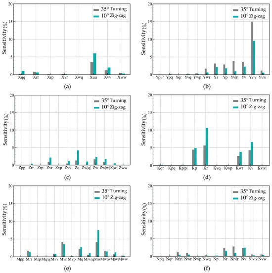
Figure 16. Sensitivity distribution of hydrodynamic coefficients in various directions. The hydrodynamic coefficients in the (a) X direction; (b) Y direction; (c) Z direction; (d) K direction; (e) M direction; (f) N direction.

Table 5. Identification results based on the Bayesian ridge regression model.

Coefficients	Bayesian × 10−4	Coefficients	Bayesian × 10−4	Coefficients	Bayesian × 10−4
X$\dot{u}$	−8.31	Z$\dot{q}$	−8.39	M$\dot{q}$	−17.2
Xuu	−11.0	Zvr	−453.8	Mq	−34.35
Xvv	171.6	Zq	−71.47	Mw	98.99
Y$\dot{v}$	−141.68	Zw	−144.05	Mvr	−5.2
Y$\dot{p}$	−5.11	K$\dot{v}$	−0.52	Mδs	−36.66
Y$\dot{r}$	4.47	K$\dot{p}$	−0.03	N$\dot{v}$	2.92
Yr	57.05	Kp	−4.8	N$\dot{r}$	−7.31
Yp	−29.7	Kr	2.6	N$\dot{p}$	−0.086
Yv|r|	4.5	Kwr	11.3	Nr	−46.31
Yv	280.76	Kv	−6.46	Nv	−145.05
Yv|v|	−1160.1	Kδr	−0.1	N|v|r	−20.8
Yδr	71.43	Z|w|	−20.0	Nδr	−26.83
Yvw	−3025.7	Zδs	−49.21
Z$\dot{w}$	−115.55	M$\dot{w}$	−2.85

Table 6 compares the hydrodynamic coefficients obtained through Bayesian ridge regression identification and through CFD simulation restraint model testing. Table 6 highlights that the hydrodynamic coefficients obtained using the Bayesian ridge regression model closely match those calculated from the CFD-constrained experiments. The Bayesian ridge regression method yielded hydrodynamic coefficients with most errors within 10%, while few exhibit larger errors, with a maximum error of −43.26%. Based on these findings, it can be concluded that identifying hydrodynamic coefficients through Bayesian ridge regression is feasible. Moreover, compared to traditional CFD methods, the identification method proposed here enables the acquiring of all hydrodynamic coefficients and offers a simple and efficient approach.

Table 6. Comparison of the hydrodynamic coefficients obtained from CFD simulation restraint model tests and Bayesian ridge regression identification.

Coefficients	CFD × 10−4	Bayesian × 10−4	Errors Compared to CFD Method %
Zw	−131.85	−144.05	9.25
Mw	95.34	98.99	3.82
Zq	−71.32	−79.43	11.37
Mq	−35.59	−34.35	−3.49
Z$\dot{w}$	−110.19	−115.55	4.87
M$\dot{w}$	−5.02	−2.85	−43.26
Z$\dot{q}$	−7.68	−8.39	9.30
M$\dot{q}$	−7.88	−7.39	−6.21
Zδs	-	−49.21	-
Mδs	-	−36.66	-
Yv	261.14	280.76	7.51
Nv	−142.96	−145.05	1.46
Kv	-	−6.46	-
Yr	57.35	57.05	−0.53
Nr	−50.20	−46.31	−7.75
Y$\dot{v}$	−139.94	−141.68	1.24
N$\dot{v}$	2.57	2.92	13.76
Y$\dot{r}$	4.32	4.47	3.47
N$\dot{r}$	−7.96	−7.31	−8.11
Yδr	-	71.43	-
Nδr	-	−26.83	-
Kδr	-	−0.10	-

4.2. Spatial Motion Prediction and Analysis

The identified hydrodynamic coefficients were updated in the motion model, and the spatial motion of the submarine was predicted. The vessel’s resulting trajectory was also obtained under the conditions, as discussed in Section 3.2. Figure 17 compares the spatial motion trajectories, showing a high level of overlap, with a maximum error of only 0.22 m. Figure 18 compares the temporal curves of the spatial motion and angular velocity components. Except for the roll angular velocity (p), the deviations within the other motion parameters are relatively small, with a maximum error of 0.089 rad/s for p. Thus, it is evident that using the Bayesian ridge regression model to identify the hydrodynamic coefficients of a submarine yields good results when predicting its spatial motion.

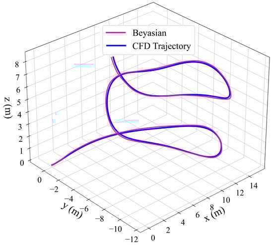
Figure 17. Comparison of the spatial motion trajectories.

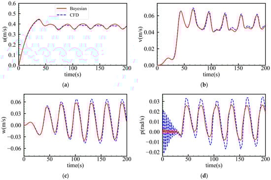
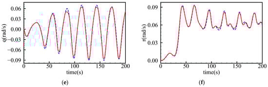
Figure 18. Comparison of time history curves for velocity and angular velocity. (a) X-direction velocity, u; (b) Y-direction velocity, v; (c) Z-direction velocity, w; (d) roll rate, p; (e) pitch rate, q; (f) yaw rate, r.

5. Conclusions

This paper proposes a new method for identifying submarine hydrodynamic coefficients based on CFD simulations of free navigation data using Bayesian ridge regression models. The developed method utilizes overset grid techniques to simulate the submarine’s multi-body movement, enabling specific sinusoidal movements of the horizontal and vertical rudders. It combines the URANS equations with a six-degree-of-freedom motion model and a body force propeller model to achieve six-degree-of-freedom free navigation of the underwater submarine. The velocity and angular velocity data are collected during the free navigation process, and the Bayesian ridge regression model is employed to identify the motion data and obtain all hydrodynamic coefficients.

This method was compared against the traditional CFD-constrained model test method, and most of the errors in the hydrodynamic coefficients were within 10%, with a maximum error of −43.26%. Furthermore, this method provides more comprehensive hydrodynamic coefficients while offering the advantages of cost-effectiveness and time efficiency.

Using the identified hydrodynamic coefficients allows the inversion of the submarine’s spatial motion, resulting in a maximum trajectory error of 0.22 m. The velocity and angular velocity profiles of the submarine’s body closely match the expected values, except for the roll angular velocity profile, which has a maximum error of 0.089 rad/s.

Currently, the submarine data are obtained through CFD simulations. Future work will conduct self-propulsion model tests using real data to identify the hydrodynamic coefficients and validate this method’s accuracy.

References

- Gertier, M.; Hagen, G.E.; Hagen, G.R. Standard Equations of Motion for Submarine Simulation; NSRDC-2510; Naval Ship Research and Development Center: Bethesda, MD, USA, 1967. [Google Scholar]
- Dantas, J.L.D.; da Silva Caetano, W.; da Silva Vale, R.T.; de Oliveira, L.M.; Pinheiro, A.R.M.; de Barros, E.A. Experimental Research on Underwater Vehicle Manoeuvrability Using the AUV Pirajuba. In Proceedings of the International Congress of Mechanical Engineering (COBEM 2013), Ribeirão Preto, Brazil, 3–7 November 2013. [Google Scholar]
- Alex, G.; Morton, G. Planar Motion Mechanism and System. U.S. Patent US3052120A, 4 September 1962. [Google Scholar]
- Burcher, R.K. Co-operative tests for ITTC mariner class ship rotating arm experiments. In Proceedings of the 12th International Towing Tank Conference 1969, Rome, Italy, 22–30 September 1969. [Google Scholar]
- Kim, H.; Akimoto, H.; Islam, H. Estimation of the hydrodynamic derivatives by Rans simulation of planar motion mechanism test. Ocean Eng. 2015, 108, 129–139. [Google Scholar] [CrossRef]
- Ji, D.; Wang, R.; Zhai, Y.; Gu, H. Dynamic modeling of quadrotor AUV using a novel CFD simulation. Ocean. Eng. 2021, 237, 109651. [Google Scholar] [CrossRef]
- Wu, X.; Wang, Y.; Huang, C.; Hu, Z.; Yi, R. An effective CFD approach for marine-vehicle maneuvering simulation based on the hybrid reference frames method. Ocean Eng. 2015, 109, 83–92. [Google Scholar] [CrossRef]
- Gao, T.; Wang, Y.; Pang, Y.; Chen, Q.; Tang, Y. A time-efficient CFD approach for hydrodynamic coefficient determination and model simplification of submarine. Ocean. Eng. 2018, 154, 16–26. [Google Scholar] [CrossRef]
- Abkowitz, M.A. Measurement of hydrodynamic characteristic from ship maneuvering trials by system identification. SNAME Trans. 1980, 88, 283–318. [Google Scholar]
- Ebrahimi, S.; Bozorg, M.; Zare Ernani, M. Identification of an Autonomous Underwater Vehicle Dynamic Using Extended Kalman Filter with ARMA Noise Model. Int. J. Robot. 2015, 4, 22–28. [Google Scholar]
- Cardenas, P.; de Barros, E.A. Estimation of AUV Hydrodynamic Coefficients Using Analytical and System Identification Approaches. IEEE J. Ocean. Eng. 2019, 45, 1157–1176. [Google Scholar] [CrossRef]
- Sajedi, Y.; Bozorg, M. Robust estimation of hydrodynamic coefficients of an AUV using Kalman and H∞ filters. Ocean Eng. 2019, 182, 386–394. [Google Scholar] [CrossRef]
- Rasekh, M.; Mahdi, M. Combining CFD, ASE, and HEKF approaches to derive all of the hydrodynamic coefficients of an axisymmetric AUV. Proc. IME M J. Eng. Marit. Environ. 2022, 236, 474–492. [Google Scholar] [CrossRef]
- Sabet, M.T.; Daniali, H.M.; Fathi, A.; Alizadeh, E. Identification of an Autonomous Underwater Vehicle Hydrodynamic Model Using the Extended, Cubature, and Transformed Unscented Kalman Filter. IEEE J. Ocean. Eng. 2018, 43, 457–467. [Google Scholar] [CrossRef]
- Deng, F.; Levi, C.; Yin, H.; Duan, M. Identification of an Autonomous Underwater Vehicle hydrodynamic model using three Kalman filters. Ocean Eng. 2021, 229, 108962. [Google Scholar] [CrossRef]
- Liang, X.; Li, W.; Lin, J.; Su, L.; Li, H. Model Identification for Autonomous Underwater Vehicles Based on Maximum Likelihood Relaxation Algorithm. In Proceedings of the Second International Conference on Computer Modeling and Simulation, Sanya, China, 22–24 January 2010; IEEE: Darmstadt, Germany, 2010; pp. 128–132. [Google Scholar]
- Zhao, R.; Xie, H.; Qiao, B. A method for identifying hydrodynamic parameters of undersea vehicle based on test data. J. Unmanned Undersea Syst. 2018, 26, 335–341. [Google Scholar]
- Zhang, G.; Zhang, X.; Pang, H. Multi-innovation auto-constructed least squares identification for 4 DOF ship maneuvering modeling with full-scale trial data. ISA Trans. 2015, 25, 186–195. [Google Scholar] [CrossRef] [PubMed]
- Dinç, M.; Hajiyev, C. Identification of hydrodynamic coefficients of AUV in the presence of measurement biases. J. Eng. Mar. Environ. 2022, 236, 756–763. [Google Scholar] [CrossRef]
- Xue, Y.; Liu, Y.; Ji, C.; Xue, G. Hydrodynamic parameter identification for ship maneuvering mathematical models using a Bayesian approach. Ocean Eng. 2020, 195, 106612. [Google Scholar] [CrossRef]
- Xu, F.; Zou, Z.J.; Yin, J.C.; Cao, J. Identification modeling of underwater vehicles’ nonlinear dynamics based on support vector machines. Ocean Eng. 2013, 67, 68–76. [Google Scholar] [CrossRef]
- Wang, Z.; Zou, Z.; Soares, C.G. Identification of ship maneuvering motion based on nu-support vector machine. Ocean Eng. 2019, 183, 270–281. [Google Scholar] [CrossRef]
- Zhang, P.; Liu, C.; Hu, K.; Zhang, J. Research of Hydrodynamic Coefficients Identification for Submarine in Vertical Motions Based on APSO. In Proceedings of the 2020 IEEE International Conference on Mechatronics and Automation, Beijing, China, 13–16 October 2020. [Google Scholar]
- Tipping, M.E. Sparse Bayesian Learning and the Relevance Vector Machine. J. Mach. Learn. Res. 2001, 1, 211–244. [Google Scholar]
- MacKay, D.J.C. Bayesian Interpolation. Neural Comput. 1992, 4, 415–447. [Google Scholar] [CrossRef]
- Groves, N.; Huang, T.; Chang, M. Geometric Characteristics of DARPA (Defense Advanced Research Projects Agency) SUBOFF Models (DTRC Model Numbers 5470 and 5471); Technical Report; David Taylor Research Center: Bethesda, MD, USA, 1989.
- Celik, I.; Ghia, U.; Roache, P.J.; Freitas, C.; Coloman, H.; Raad, P. Procedure of Estimation and Reporting of Uncertainty Due to Discretization in CFD Applications. J. Fluids Eng. 2008, 130, 078001. [Google Scholar]
- Dantas, J.L.D.; de Barros, E.A. Numerical analysis of control surface effects on AUV manoeuvrability. Appl. Ocean Res. 2013, 42, 168–181. [Google Scholar] [CrossRef]
- Menter, F.R. Two-Equation Eddy-Viscosity Transport Turbulence Model for Engineering Applications. AIAA J. 1994, 32, 1598–1605. [Google Scholar] [CrossRef]
- Liu, H.-L.; Huang, T. Summary of DARPA Suboff Experimental Program Data; Naval Surface Warfare Center, Carderock Division (NEWCCD): Bethesda, MD, USA, 1998; Volume 28.
- Zhang, N.; Shen, H.; Yao, H. Uncertainty analysis in CFD for resistance and flow field. J. Ship Mech. 2008, 12, 211. [Google Scholar]
- Han, K.; Cheng, X.; Liu, Z.; Huang, C.; Chang, H.; Yao, J.; Tan, K. Six-DOF CFD Simulations of Underwater Vehicle Operating Underwater Turning Maneuvers. J. Mar. Sci. Eng. 2021, 9, 1451. [Google Scholar] [CrossRef]
- Oda, J.; Yamazaki, K. Technique to Obtain Optimum Strength Shape by the Finite Element Method: On Body Force Problem. Trans. Jpn. Soc. Mech. Eng. 1978, 44, 1141–1150. [Google Scholar] [CrossRef][Green Version]
- Yeo, D.J.; Rhee, K.P. Sensitivity analysis of submersibles’ maneuverability and its application to the design of actuator inputs. Ocean Eng. 2006, 33, 2270–2286. [Google Scholar] [CrossRef]
Disclaimer/Publisher’s Note: The statements, opinions and data contained in all publications are solely those of the individual author(s) and contributor(s) and not of MDPI and/or the editor(s). MDPI and/or the editor(s) disclaim responsibility for any injury to people or property resulting from any ideas, methods, instructions or products referred to in the content. |
© 2023 by the authors. Licensee MDPI, Basel, Switzerland. This article is an open access article distributed under the terms and conditions of the Creative Commons Attribution (CC BY) license (https://creativecommons.org/licenses/by/4.0/).