Article

Macro–Micro-Coupled Simulations of Dilute Viscoelastic Fluids

1
School of Mathematics and Statistics, Rochester Institute of Technology, Rochester, NY 14623, USA
2
Department of Mathematics, University of South Carolina, Columbia, SC 29208, USA
*
Author to whom correspondence should be addressed.
Appl. Sci. 2023, 13(22), 12265; https://doi.org/10.3390/app132212265
Submission received: 3 October 2023 / Revised: 30 October 2023 / Accepted: 8 November 2023 / Published: 13 November 2023
(This article belongs to the Special Issue Multiscale Modeling of Complex Fluids and Soft Matter)

Abstract

:
Modeling the flow of polymer solutions requires knowledge at various length and time scales. The macroscopic behavior is described by the overall velocity, pressure, and stress. The polymeric contribution to the stress requires knowledge of the evolution of polymer chains. In this work, we use a microscopic model, the finitely extensible nonlinear elastic (FENE) model, to capture the polymer’s behavior. The benefit of using microscopic models is that they remain faithful to the polymer dynamics without information loss via averaging. Their downside is the computational cost incurred in solving the thousands to millions of differential equations describing the microstructure. Here, we describe a multiscale flow solver that utilizes GPUs for massively parallel, efficient simulations. We compare and contrast the microscopic model with its macroscopic counterpart under various flow conditions. In particular, significant differences are observed under nonlinear flow conditions, where the polymers become highly stretched and oriented.

1. Introduction

Viscoelastic fluids are materials that exhibit complex behaviors due to their unique composition and structure. Uses of these materials can be found in many industrial, biomedical, and basic science applications [1,2,3,4,5,6]. Common examples include liquid crystals, polymers, and colloids. In practice, modeling the behavior of viscoelastic materials requires significant computational power, which clashes with the need for fast simulations. An increasing number of research studies focus on the mathematical modeling of viscoelastic fluids at different scales. To allow such modeling efforts to be useful in practice, there is a critical need for more efficient computational methods. In recent years, GPU computing has emerged as a valuable tool to overcome these challenges. Here, we describe numerical algorithms aimed at using GPU computing in viscoelastic flow simulations.
GPU computing refers to the use of graphics processing units (GPUs) to perform numerical computations. GPU computing has become an important tool for the study of complex fluids due to its ability to handle large amounts of data and perform computations in parallel. Because GPUs can handle massive computational demands, they can provide results in a fraction of the time of traditional CPU-based methods. As computing power continues to increase, GPU-based simulations can become increasingly important for understanding the behavior of complex materials and complex flows. GPUs have been previously used in the modeling of polymeric systems. Reith et al. [7] performed numerical simulations to find the equilibrium properties of polymer rings. Brito et al. [8] used GPUs to accelerate computations of smoothed particle hydrodynamics (SPH) for viscoelastic materials. Ingelsten et al. [9] extended their Lagrangian–Eulerian method for viscoelastic flow simulations to GPU computing. Yang et al. [10] simulated phase separation in polymer blends and polymer solutions using a GPU-based viscoelastic model. Bergamasco et al. [11] introduced a lattice-Boltzmann-based finite-volume formulation, where the macroscopic equations were solved by a finite-volume method and the microscopic equation was solved by a lattice-Boltzmann method. These authors implemented the solution to the microscopic equation in GPUs. Gutierrez-Castillo et al. [12] used GPUs to accelerate their three-dimensional numerical simulations of viscoelastic fluids for both the Oldroyd-B and FENE-P models. Schram and Barkema [13] simulated ring polymer melts via GPU computing using an elastic lattice polymer model. Behbahani et al. [14] investigated high-molecular-weight entangled polymer melts using HOOMD-blue, a GPU accelerated simulation software. In this paper, we use GPU computing to couple dynamics at the macroscale with those at the mesoscale, described by Langevin-type equations.
From a modeling perspective, it is well-known that the stress, τ , of any Newtonian fluid is directly proportional to the imposed shear rate, τ = η γ ˙ , where the proportionality constant η is the viscosity of the material. Differences between materials will only affect the value of η but not the functional form of the constitutive equation. Mathematically speaking, this means that for Newtonian fluids, there is a single, general constitutive equation capable of describing different types of Newtonian materials. In principle, this means that the same numerical algorithms can be used for any material by only changing the value of the viscosity constant. In contrast, there is not a single all-encompassing constitutive equation for viscoelastic materials. This is because, in this case, the evolution of the stress as a function of the applied strain can vary from material to material or even for the same material under different flow conditions. Accordingly, the formulation of constitutive equations describing different types of viscoelastic materials is a prolific area of research [15]. It is not surprising, then, that because of the lack of a single constitutive equation and due to their ubiquity in many industrial and biological processes, numerical methods for solving the flow of these viscoelastic materials under flows fields of different levels of complexity have been a very active research field. Some extensive reviews in this subject can be found in [9,16,17,18,19,20].
Broadly speaking, the link between polymer fluids and external fields is relatively well-understood: how a polymeric fluid behaves under a given field is directly governed by the dynamics of their corresponding underlying microstructure. For polymeric fluids, this microstructure comprises polymer chains. The underlying dynamics include coiling and uncoiling processes, hindered motion due to physical entanglements or hydrodynamic effects caused by the presence of other polymer molecules in their vicinity, and in some cases, physical cross-linking between chains. In this paper, we focus on a subclass of the available computational techniques: the so-called micro–macro approaches [18]. These approaches combine the solution of the conservation equations at the macroscale with models derived from kinetic theory at the microscale. The advantage of using kinetic models is that instead of a homogenized view of the rheology of the material through a macroscopic constitutive equation, the viscoelastic contribution to the stress is obtained using coarse-grained representations of the microstructural dynamics. For more comprehensive reviews on these methods, the reader is referred to [18,21,22,23,24,25].
Micro–macro methods are especially appealing when modifications to the microstructural dynamics need to be introduced without incurring large numerical changes or extreme computational costs. This is because the evolution of the microscopic description is somehow decoupled from the macroscopic flow solvers. This has the potential of making the model highly versatile and applicable to a range of deformation conditions. In addition, micro–macro methods facilitate the investigation of the effects of various parameters to gain insights into the underlying physics of a given phenomenon and lead to an optimization of a range of industrial processes. On the other hand, micro–macro methods are more computationally demanding than their corresponding macroscopic counterparts. In practice, one must choose between models that are computationally tractable but perhaps do not offer a direct link between the flow-induced development of the micro-structure and the applied flow field or be limited to simple geometries and viscometric flows when using macro–micro methods.
Within the context of microscopic models, different models have been developed to describe the coupling between macroscopic response and microstructure dynamics in polymeric fluids. One family of models are the so-called bead-spring models. These models use molecular coarse-graining to describe the behavior of polymer chains represented as beads connected by massless springs. The simplest of these models considers only two beads, and it is known as the elastic dumbbell model. Although it is widely recognized that a single dumbbell is too simple to be able to describe any complicated dynamics in polymeric systems, it is also known that stretching and orientation alone suffice to give a qualitative description of steady-state rheological properties and flows with slow characteristic time scales [15]. Accordingly, these models have been extensively used to develop “an elementary but broad understanding of the relation between macro-molecular motions and rheological phenomena” [15]. One of the most common dumbbell models is the Hookean dumbbell model, where the spring connecting the two beads is assumed to follow a linear elastic law ( Hooke’s law). This model, although physically unrealistic, has the advantage of being the only model in its class with an exact closure [15,26]; this closure leads to the well-known macroscopic constitutive equation called the Oldroyd-B model. If a different spring law is assumed, the transition between micro and macro models is not directly possible. For instance, the family of models derived from using a finite extensible (FENE) spring force can have many types of closure depending on which approximation is made in the closure step. Many studies have investigated the effects of the different FENE closures; for an example, see Herrchen and Öttinger [27].
In short, the use of dumbbell models allows for the simulation of complex fluids at a molecular level, which, although somewhat unrealistic, can still provide valuable insight into the microstructural responses in these materials. However, simulating complex fluids using dumbbell models requires large amounts of computational power, which has hindered the ability to conduct large-scale simulations until recently. That is why, although some information is lost by averaging the effect of the dumbbells in a single differential equation, macroscopic models are still more widely used in complex flow. The main reason for this is that PDE models are more computationally tractable than their SDE counterparts. Parallel computing has surfaced as an alternative to close the gap between these two computational costs. In particular, GPU computing emerged in past decades as a cheap option for performing parallel computing. The only drawback when dealing with GPUs is that memory transfer between the CPU and the GPU is very costly, which is why these devices perform better on systems that are trivially parallelizable.
Here, we demonstrate the use of GPU computing using non-interacting dumbbell models, which are by design trivially parallelizable. First, we explore two viscometric flows: simple shear and uniaxial extensional flow. Next, we show the coupling between an existing macro solver [28] and the GPU dumbbell models to simulate capillary thinning. Capillary thinning is a phenomenon where a liquid bridge formed between two solid surfaces undergoes thinning due to surface tension forces until it breaks. This is a common phenomenon in a variety of industrial processes, such as coating, printing, and microfabrication [1,3,5]. The use of simulations in understanding capillary thinning can provide insight into the underlying physics and aid in the design of improved processes. An advantage of using dumbbell models is that they enable the investigation of the effects of various microstructural parameters on capillary thinning.

2. Governing Equations

2.1. Macroscopic Flow Equations

At the macroscale, considering an unsteady, incompressible viscoelastic flow and in the absence of external body forces, the flow is governed by the conservation of mass and the conservation of momentum equations
˜ · u ˜ = 0 ,
ρ u ˜ t ˜ + u ˜ · ˜ u ˜ = ˜ p ˜ + η s ˜ 2 u ˜ + ˜ · τ ˜ ,
where u ˜ is the velocity vector, p ˜ is the pressure, τ ˜ is the extra stress tensor, η s is the solvent viscosity, and ρ is the density.
We scale the conservation equations as follows:
t = t ˜ · U L , x = x ˜ · 1 L , u = u ˜ · 1 U , p = p ˜ · 1 ρ U 2 , τ = τ ˜ · λ η p .
Here, L is a characteristic macoscopic length, U is a characteristic velocity, η p is the zero shear rate polymeric viscosity, and λ is the longest relaxation time. With this scaling, the conservation equations become
· u = 0 ,
u t + u · u = p + 1 R e β 2 u + 1 β D e · τ .
Several nondimensional groups arise from this scaling:
  • The Reynolds number, R e = ρ U L η , which is the ratio of inertial to viscous forces.
  • The ratio of the solvent to total zero-shear viscosity: β = η s η s + η p .
  • The Deborah number, D e = λ U L , which is the ratio of the fluid relaxation time to a characteristic time for the macroscopic flow. Note that in the case of viscometric flow, in which U / L = γ ˙ 0 , this is also referred to as the Weissenberg number.

2.2. Constitutive Equations for Extra Stress

To solve the resulting system of conservation equations, an expression for the extra stress tensor, τ , is necessary. As discussed in the introduction, there are several ways in which the extra stress can be modeled. Here we use a micro–macro approach [21], where the coarse-grained approximation at the mesoscale utilizes non-interacting elastic dumbbells. Below, we introduce the evolution equations of the dumbbell models used in this study. For completeness, we also introduce the macroscopic closure equations corresponding to each of the two dumbbell models considered.

2.2.1. Microscopic Description—Dumbbell Models

The solvent is assumed to be an incompressible Newtonian fluid of viscosity η s . The configuration of the dumbbell, shown in Figure 1, is described by the end-to-end connector vector Q = r 2 r 1 and the center-of-mass vector r c = 1 2 r 1 + r 2 . Here, we assume a homogeneous distribution, so that the only variable of =interest is Q .
The stochastic differential equation describing the evolution of the end-to-end vector is given by [15,29],
d Q ˜ t = ˜ u ˜ · Q ˜ t 2 ζ F Q ˜ t + 4 k B T ζ d W t ,
where F ( · ) denotes the functional form of the spring force, W t is a two-dimensional Wiener process, ζ is the drag coefficient acting on each bead, and k B T is the thermal energy.
The viscoelastic contribution to the stress is given by Kramer’s relation [15,29],
τ ˜ = n F ( Q ˜ ) Q ˜ n k B T I ,
where n is the dumbbells’ number density, n F ( Q ) Q is the contribution of the tension on the spring with the spring law F ( Q ) , and n k B T captures effects due to Brownian motion.
  • Hookean dumbbells:
    For Hookean dumbbells, a linear form is assumed for the spring force, F ( Q ) = H Q , where H is the spring constant. With this, Equations (5) and (6) become
    d Q ˜ t = ˜ u ˜ · Q ˜ t 2 H ζ Q ˜ t + 4 k B T ζ d W t ,
    τ ˜ = n H Q ˜ Q ˜ n k B T I .
    These equations are scaled using Equation (3) and the characteristic microscopic length,
    x = k B T H .
    With these,
    η p = n k B T λ , τ = τ ˜ · λ η p = τ ˜ · 1 n k B T , Q = Q ˜ · H k B T .
    In addition, the longest relaxation time is defined as
    λ = ζ 4 H .
    The resulting non-dimensional equations are then
    d Q t = u · Q t 1 2 D e Q t + 1 D e d W t ,
    τ = Q Q I ,
    where the Deborah number is defined as before, D e = λ U / L .
  • FENE Dumbbells
    If instead of a linear spring connector a finitely extensible spring is considered, we obtain FENE-type models. These models are derived by introducing Warner’s finitely extensible nonlinear connector force law [15],
    F Q ˜ = H Q ˜ 1 Q ˜ / Q max 2 ,
    where Q 2 = Q · Q and Q max is the maximum allowed extension of the dumbbell.
    Introducing this spring law into Equation (5) and non-dimensionalizing as before gives
    d Q t = u · Q t 1 2 D e Q t 1 Q 2 / b + 1 D e d W t ,
    τ = Q Q 1 Q 2 / b I ,
    where the nonlinear FENE parameters are b = H Q max 2 / ( k B T ) .

2.2.2. Macro-Constitutive Equations—Closure Models

In this section, we introduce macroscopic closures for the two dumbbell models discussed in Section 2.2.1. We introduce these closures here and use them in Section 3.1 and Section 3.2 to compare their results with those of their corresponding microscopic dumbbell model. The main objective is to show how much information is lost at the microscale using closure approximations. These shortcomings of the macroscopic closures highlight the importance of micro–macro models to properly capture the underlying dynamics that govern the flow in complex fluids.
Recall that the extra stress is found as a function of the second moment of the end-to-end vector, Q . From the equation of motion of a dumbbell, Equation (5), the following evolution equation for the second moment of the end-to-end vector Q can be derived:
Q ˜ Q ˜ ( 1 ) + 4 ζ F ( Q ˜ ) Q ˜ = 4 k B T ζ I ,
where ( · ) ( 1 ) is the upper convected derivative, defined as
( · ) ( 1 ) = ( · ) t + u · ( · ) ( · ) · u u · ( · ) .
  • Upper convected Maxwell model:
    If the spring is linear (Hookean), where F ( Q ) = H Q , the resulting constitute equation obtained from Equation (14) is known as the upper convected Maxwell (UCM) model
    τ ˜ = n H Q ˜ Q ˜ n k B T I ,
    Q ˜ Q ˜ ( 1 ) + 4 H ζ Q ˜ Q ˜ = 4 k B T ζ I .
    Using the same scaling as before leads to the following non-dimensional constitutive equations:
    τ = Q Q I ,
    D e Q Q ( 1 ) + Q Q = I .
  • FENE-P model
    In a FENE model, with the spring law given by Equation (12), the evolution equation, Equation (14), becomes
    Q ˜ Q ˜ ( 1 ) + 4 H ζ H Q ˜ Q ˜ 1 ( Q ˜ / Q max ) 2 = 4 k B T ζ I .
    Different FENE models can be formulated based on the approximation used to calculate the second term in Equation (18). Here, we focus on the FENE-P model, which is obtained by the approximation
    H Q ˜ Q ˜ 1 ( Q ˜ / Q max ) 2 = Q ˜ Q ˜ 1 Q ˜ 2 / Q max 2 .
    With this approximation, the constitutive equations become
    τ ˜ = n H 1 Q ˜ 2 / Q ˜ max 2 Q ˜ Q ˜ n k B T I ,
    Q ˜ Q ˜ ( 1 ˜ ) + 4 H ζ Q ˜ Q ˜ 1 Q ˜ 2 / Q ˜ max 2 = 4 k B T ζ I .
    Scaling as before, we obtain
    τ = Q Q 1 Q 2 / b I ,
    D e Q Q ( 1 ) + Q Q 1 Q 2 / b = I .
    For convenience, one can define the non-dimensional configuration tensor, A , as
    A d Q ˜ Q ˜ Q ˜ 2 0 ,
    where Q ˜ 2 0 is the mean-square end-to-end spring length at equilibrium (absence of flow) and d is the dimensionality [15].
    Note that if we scale the end-to-end vector as before, we have
    A d k B T H Q Q Q ˜ 2 0 = d Q Q k B T H Q ˜ 2 2 = d Q Q 1 d = Q Q .
    In addition, trace A = d Q 2 .
    The constitutive equation for A in two dimensions is
    τ = A 1 trace A / ( 2 b ) I .
    D e A ( 1 ) + A 1 trace A / ( 2 b ) = I ,

2.3. Numerical Considerations

In this work, we use graphics processing units (GPU) to perform calculations at the mesoscale. This approach takes advantage of the fact that the stochastic differential equations for non-interacting dumbbells are trivially parallelizable, so that one can concurrently solve millions of equations. This approach eliminates the need for variance reduction approaches [30,31,32] since it is possible to resolve hundreds of thousands of realizations with very little computational time. The main computational scheme is summarized in Figure A1, particular considerations for the Hookean and FENE dumbbells are described below.
One thing to keep in mind when using GPUs is that this approach works best when the dynamics of the individual dumbbells are trivially parallelizable. That is why, for instance, modeling hydrodynamics comes with a much higher computational costs using GPUs. In this study, we limit ourselves to equations of motion that are trivially parallelizable.
  • Parameter values: Unless otherwise noted, the parameter values used in the simulations are given in Table 1.
Table 1. Simulation parameters.
ParameterSymbol—EqnUnitsValueRef.
Density ρ kg/m 3 1000
Solvent viscosity η s Pa s0.001
Zero shear rate viscosity η 0 = η s + η p Pa s0.0037[33]
Characteristic relaxation time λ s0.010[34]
Characteristic velocity U = γ / ( ρ R 0 ) m/s0.260
Characteristic lengthLm0.003
Surface tension γ N/m0.070[34]
Initial jet radius R 0 m0.001[34]
Reynolds number R e = ρ U L / η 0 Dimensionless78
Ratio of viscosities β = η s / η 0 Dimensionless0.270
Deborah number D e = λ U / L Dimensionless0.800
Ohnesorge number O h = η 0 / ρ γ R 0 Dimensionless0.038
FENE parameterbDimensionless 10 5
WavenumberkDimensionless0.8

2.3.1. Hookean Dumbbells

Equation (11a) will be solved for each dumbbell using a forward Euler scheme,
Q t j + 1 = Q t j + u · Q t j 1 2 D e Q t j Δ t j + 1 D e Δ W j .
Boundary conditions for Q are imposed at the macroscale through u . Whenever necessary to calculate the stress gradient, ghost cells will be included in the macroscale grid.

2.3.2. FENE Dumbbells

Because of the nonlinearity introduced in the evolution equation, a semi-implicit, first-order algorithm is used instead of the forward Euler scheme. Briefly, a two-step operator splitting procedure is implemented, where the two steps are given by Equations (26) and (27) [29] as follows:
Q ¯ t j + 1 = Q t j + u · Q t j 1 2 D e Q t j 1 Q t j 2 / b Δ t j + 1 D e Δ W j ,
and
1 + 1 4 D e Δ t j 1 Q 2 t j + 1 b Q t j + 1 = Q t j + 1 D e Δ W j + 1 2 [ u t j + 1 · Q ¯ t j + 1 + u t j · Q t j 1 2 D e Q t j 1 Q 2 t j b ] Δ t j .
Equation (27) can be written as
Q j + 1 3 P Q j + 1 2 b 1 + 1 4 D e Δ t Q j + 1 b P = 0 ,
where P is the magnitude of the right-hand side of Equation (27). This cubic equation has one real root in the interval 0 , b [29,35]. The approach is to find the magnitude of Q t j + 1 using the polynomial’s solution in this interval; then, its direction is found by solving Equation (27) for each vector component.
Note that Equation (27) requires the velocity gradient tensor, u t j + 1 , at time t + 1 , which is unknown for non-viscometric flows. In our computations, u t j + 1 is found by a second-order extrapolation following [35],
u t j + 1 = 2 u t j u t j 1 .

3. Results

3.1. Simple Shear

This flow field results from placing the fluid between two parallel plates, with the lower plate stationary and the upper plate moving at a constant velocity U top . Under viscometric conditions, the equations can be simplified by assuming a fully developed flow so that
u ˜ = γ ˙ 0 y ˜ , 0 , · x = 0 ,
where γ ˙ 0 = U top / L and L is the plates’ separation.
Using the same scaling as before simplifies the velocity to u = y , 0 , and the velocity gradient tensor reduces to
u = 0 1 0 0 .
All initial conditions correspond to equilibrium conditions. For dumbbell models, this means the end-to-end vectors are drawn from a normal distribution. For the closure models, this means the extra stress is zero.
The UCM model is an exact closure of the Hookean dumbbell equation, and as expected results from these two models will always agree, this is confirmed in Figure 2, where results from both models in viscometric simple shear flow are compared.
Similarly, Figure 3 compares results from the FENE-P model with stochastic simulations of FENE dumbbells. The figure shows that the FENE-P approximation underpredicts the nonlinear behavior of the shear stress, in agreement with previous studies [27].
Figure 4 shows that as the nonlinearity, represented by the parameter b, is increased, the discrepancies between the micro and macro representations become more pronounced. For a more in-depth comparison between the FENE model and different FENE closures, the reader is referred to [27].
The advantage of using dumbbell equations, as opposed to closure approximations, is that in addition to the average stress behavior, shown in Figure 2, Figure 3 and Figure 4, one can also capture the stretching and orientation of dumbbells under flow. In this way, the model predictions can be compared to data obtained from scattering techniques [36]. Figure 5 shows the temporal evolution of the distribution of dumbbell lengths, Q x vs. Q y , as a function of shear flow both in the linear regime, D e = 10 , and the nonlinear regime, D e = 500 . In the linear regime, dumbbells are stretched and oriented in the direction of the flow, but the distribution of lengths remains Gaussian. In the nonlinear regime, Gaussianity is lost around the same time the overshoot in the shear stress is observed.
We can also examine the probability distribution function of the dumbbell orientation as a function of the Deborah number; these results are shown in Figure 6. The figure shows that the nonlinear behavior differs from linear behavior in two main ways. First, the ‘molecules’ are more oriented with respect to the flow, as proven by the fact that the mean orientation angle at steady state for D e = 10 is not quite zero, while for D e = 500 , the mean angle is zero. Second, narrower distributions for D e = 500 indicate that more ‘molecules’ are aligned with the flow at steady state compared with molecules in the linear regime.
A final checkpoint for our simulations is the expansion ratio, defined as
e = e x 2 + e y 2 2 ,
where the axes of extension for the dumbbell ‘molecule’ are calculated as
e i = Q i 2 Q i 2 0 , i = x , y
where < · > 0 represents the mean deformation at equilibrium.
Figure 7 shows the expansion ratio for different values of D e . Compared to the information gathered from the shear stress curves, the expansion ratio does not offer any new insight into the flow dynamics. However, our simulations at the mesoscale allow us to take a closer look at the individual axes of extension and analyze their behavior, as shown in Figure 8.
In Figure 8, we show the particulars of the two axes of extension in the nonlinear regime, D e = 500 , together with their distributions at some selected times. In the scattering plots, we have normalized the axes with respect to their maximum values. However, we should note that the maximum values vary widely for different times. For instance, at t = 1 : max e x = 10.54 , while at t = 1000 : max e x = 295.82 . This normalization was carried out to visualize the breaking of isotropy in the stretching as the system approaches the stress overshoot.

3.2. Elongational Flow

This flow field results from stretching the fluid in one direction at a rate ε ˙ 0 = d ε / d t , where ε is the strain. As before, we assume a fully developed flow so that the velocity field is given by
u ˜ = ε ˙ 0 x ˜ , 1 2 ε ˙ 0 y ˜ , 1 2 ε ˙ 0 z ˜ .
Using the same scaling as before simplifies the velocity as u = x , 1 2 y , 1 2 z and the velocity gradient tensor as
u = 1 0 0 0 1 2 0 0 0 1 2 .
As before, we assume that initially, the system is at equilibrium, as discussed in Section 3.1.
Figure 9 shows the comparison of the macro and stochastic simulations. As expected, the FENE-P closure deviates from the FENE dumbbell model, and this deviation increases in the nonlinear regime. For a complete discussion of FENE models under rapid elongational flow, the reader is referred to [37].

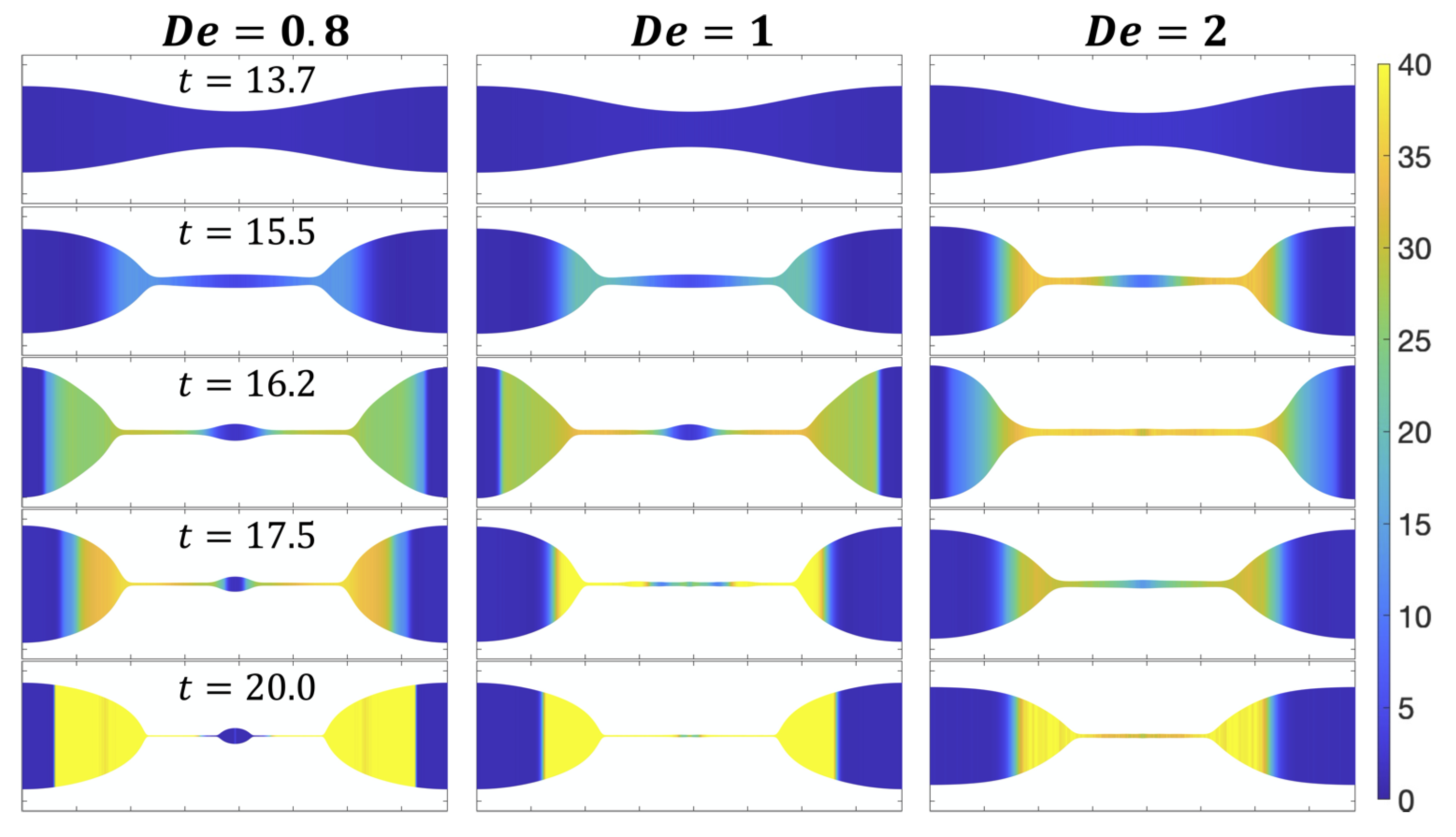
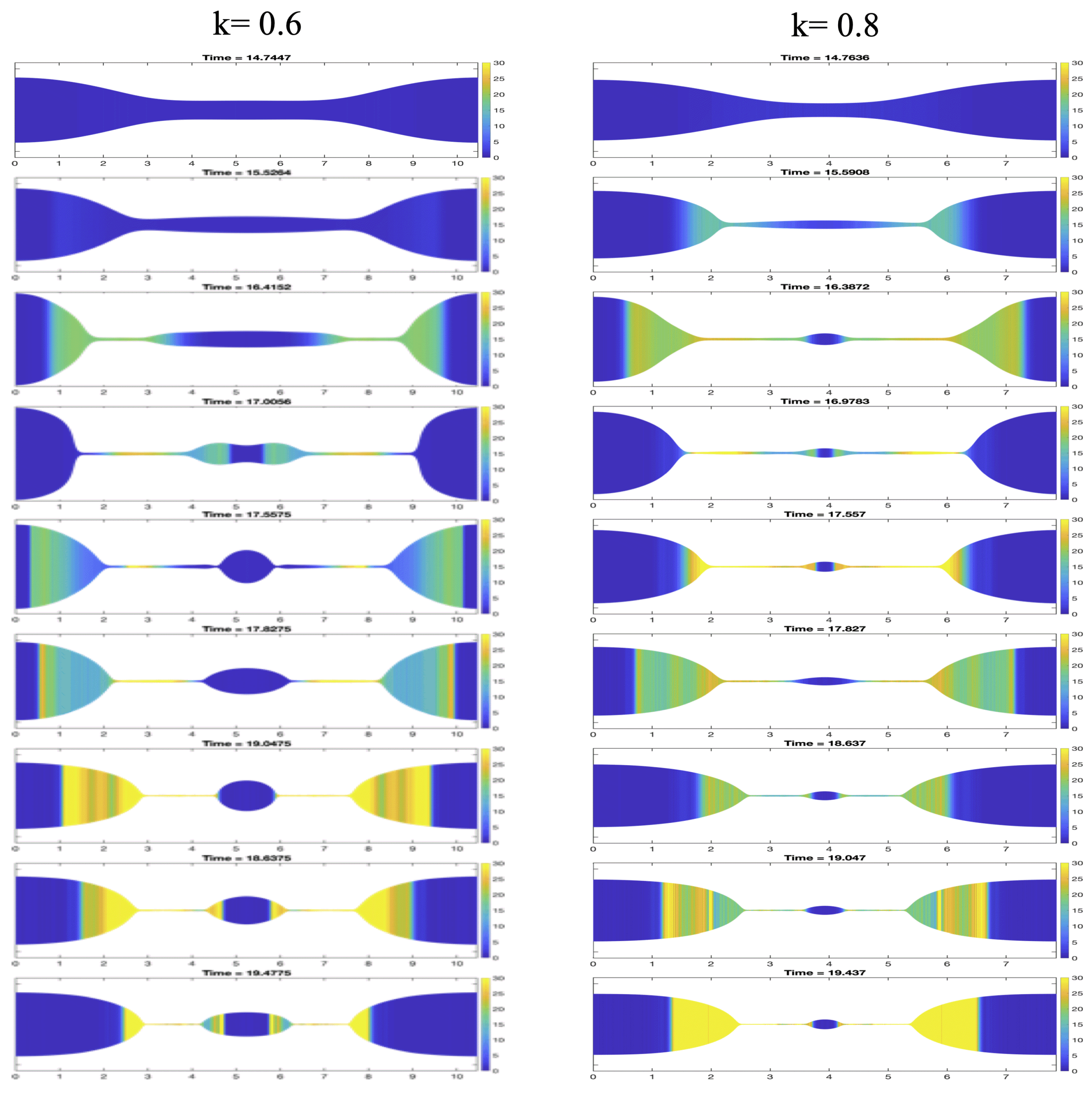
3.3. Capillary Thinning

Transient elongational rheometry is used to obtain comparative information about the elongational behavior of polymer solutions. The investigation of the elongational behavior of complex fluids is relevant to applications defined by spraying and jetting, such as microfluidic devices, printing, fiber spinning, and understanding how droplet emissions from respiratory events affect the transmission of infectious diseases [1,2,3,4,5,6]. Ardekani et al. [34] showed that three conditions should be satisfied for an elongational experiment to be successful: an elastocapillary balance must be established, the range of diameters of the liquid jets should be experimentally accessible, and the formation of secondary droplets along the thread must be suppressed. Clearly, understanding the underlying microstructural dynamics that govern one or more of these conditions is important to evaluate the optimal performance both under experimental and application settings. While most of the theoretical analysis is carried out using homogenized views of the microstructure in the form of macroscopic constitutive equations, using methods that allow for the straightforward explicit integration of microstructural dynamics is appealing. Here, our goal is to illustrate how coarse-grained mesoscopic simulations can also be used to gain insight into the development of droplets in a viscoelastic fluid jet. We note that the objective of this publication is to demonstrate the feasibility of the methods, and we take advantage of symmetry and one-dimensional flow fields to simplify many of the computations. More in-depth studies will be left for future investigations.
In capillary thinning experiments, a piece of fluid is stretched between two separating surfaces, with surface tension being the main driver of the fluid motion. When a Newtonian fluid is stretched, its radius decreases due to surface tension until it breaks into many droplets. For viscoelastic materials, the underlying microstructure can give rise to different configurations. In polymeric materials, these dynamics involve nonlinear effects derived from the finite extensibility of polymer chains within the fluid. As the fluid jet starts to form droplets, the polymer inside the drops remains relaxed, while polymer chains in the filaments between drops become strongly oriented and stretched, essentially leading to the formation of bridges with high tensile strains. This instability, characteristic of fluids that have some elasticity, has become known as a “beads-on-a-string” structure [38,39,40,41]. Moreover, under certain flow regimes, when there is a balance of capillary, viscous, and inertial effects, additional structures can appear. For a more in-depth review of the formation of bead-on-a-string structures, see [40].
To solve this flow, a thin film formulation is used where only the leading-order approximation in an expansion on the jet radius, R ( z , t ) , is considered [42]. This essentially assumes that the flow inside the fluid jet is one-dimensional so that the only relevant variables are the radius and the axial velocity, v ( z , t ) . In this case, the non-dimensional conservation of mass and of momentum equations are simplified as [43],
R 2 t + z ( v R 2 ) = 0
v t + v v z = κ z + 3 O h β R 2 z R 2 v z + O h D e 1 β R 2 z R 2 ( τ z z τ r r ) ,
where
κ = 1 R 1 + R z 2 1 / 2 R z z 1 + R z 2 3 / 2
is the curvature and τ is the polymer contribution to the stress. The equations have been non-dimensionalized by taking the initial radius of the jet, R 0 , as the characteristic macroscopic length scale and the Rayleigh time, t R = ρ R 0 3 / γ , as the macroscopic characteristic time scale; this gives the characteristic velocity as γ / ( ρ R 0 ) . Finally, the Ohnesorge number is defined as O h = η 0 / ρ γ R 0 , and all other dimensionless groups are defined as before.
With this scaling, the dynamics of the axisymmetric slender jet are governed by three non-dimensional groups: the Ohnesorge number, O h , which is the ratio of surface tension to inertial forces; the parameter β , which is the ratio between the solvent and fluid viscosities; and the Deborah number, D e , which measures the ratio of the material’s characteristic time to the time scale of the flow. An additional parameter captures the nonlinear viscoelastic behavior of the polymer chains, which, in the case of FENE models, is the finite extensibility parameter, b, defined above.
The nonlinear system of partial differential equations (PDEs), Equation (36), is solved numerically via finite differencing [28]. All spatial terms, except convection, are discretized using second-order central differencing. For the convective terms, a velocity-weighted upwind discretization scheme is used. In particular, the derivative is interpolated between pure central differencing and pure upwind. The result is that in regions of slow flow, a central differencing is used; however, as the velocity increases, the weighting moves closer to a pure upwind differencing. For the convective terms where the derivative depends on the velocity, the first derivative is calculated as follows:
f z j = ( 1 g j ) ( f j + 1 f j ) 2 Δ z + ( 1 + g j ) ( f j f j 1 ) 2 Δ z ,
where g j = v j / v m a x .
We use the implicit Euler method for time discretization combined with time filters, which increase the order of accuracy from first to second order [44]. Additionally, we have implemented variable step sizes, which greatly enhances the speed and efficiency of the solver. The numerical solver has been benchmarked against existing simulations of the Oldroyd-B model [34].
In the spatial domain, periodic boundary conditions are used for the velocity, the radius, and the polymer configurations. The initial condition considers a homogeneous base state corresponding to a uniform cylindrical shape and molecules at equilibrium conditions. To this base state a small amplitude perturbation is added. We note that the eigenvalues of the linearized system resulting from expanding the governing equations to first order in the amplitude of these perturbations determines how fast the perturbations grow towards a necked state or whether they decay to leave a uniform filament. Following [34], we set the initial shape of the jet as
R = R 0 1 + 0.01 cos k z ,
where k is the wavenumber.
At each time step, the system of PDEs is solved to find the velocity field. The field is then used to find the velocity gradient, u , at each grid point. Using these values, the dumbbell configurations are updated using Equation (13a) and the extra stress calculated with Equation (13b). The resulting values for the extra stress at each grid point are introduced in the macroscopic simulation through Equation (36b).
Below, we show the results obtained when the Deborah number, the wavelength values, and the maximum extensibility of the FENE dumbbells are varied. As a metric for microstructural organization, we use the expansion ratio defined in Equation (32).

3.3.1. Deborah Number

Figure 10 shows the evolution of the jet morphology as a function of the Deborah number, D e . As the elasticity of the fluid is increased—a larger D e —the formation of droplets is inhibited. This inhibition is related to the higher tensile stress in the filament prior to the formation of the droplets, represented by a larger expansion ratio in the figures. This, in turn, hinders the reorganization of the strands that would result in a lower expansion ratio in the middle of the jet, which is what ultimately leads to the formation of droplets.

3.3.2. Wavelength

The effect of the excitation wavenumber on the formation of droplets is well understood; see, for example, [34,45,46,47]. Briefly, there are three regimes: (i) for very small wavelengths, the jets are characterized by traveling capillary waves; (ii) in the middle regime, the jet develops single and multiple drops; and (iii) at large wavelength numbers, no formation of droplets is observed. Our simulations show the same behavior. In Figure 11 the jet evolutions for two different wavenumbers are shown. The expansion ratio shows the same trends discussed above, where the main stretching is observed at the bridges. In addition, this figure shows that smaller droplets result in a higher level of stretching in other regions of the filament.

3.3.3. Nonlinear FENE Parameter

Figure 12 shows the evolution of droplets for two values of the nonlinear parameter b. Recall that b controls the maximum stretch allowed in the dumbbells. It is this stretch that gives polymer solutions their elasticity. In this manner, filament formation has a similar trend when varying b and D e , i.e., as maximum extensibility is increased, satellite bead formation is suppressed. Under conditions where satellite beads do form, smaller, secondary droplets between the satellite and main beads may appear. As shown in Figure 12, larger values of b suppress these secondary droplets. Furthermore, another main difference is observed at the pinch sites, with smaller values of b resulting in more pronounced pinching. This is a result of less elasticity, hence more viscous-like behavior.

4. Discussion

In this work, we have considered multiscale simulations of dilute polymeric solutions under homogeneous and non-homogeneous flow conditions. At the microscale, Langevin equations describing the behavior of elastic dumbbells are solved using GPUs, which allows for massively parallel simulations. Considering dumbbell equations provides more accurate information on the stretch and orientation of polymer chains, as opposed to macroscopic constitutive equations. In this way, the stretching and orientation of dumbbells are captured in a similar manner in which an experimentalist will analyze fluid behavior using scattering techniques.
Under viscometric conditions of simple shear and uniaxial extension, we showed that there is a significant difference between predictions from macroscopic and mesoscopic models. These differences are exacerbated under nonlinear flow conditions. In the linear regime, dumbbells are stretched and oriented in the direction of the flow, but the distribution of lengths remains Gaussian. In the nonlinear regime, Gaussianity is lost around the same time the overshoot in the shear stress is observed. Furthermore, the PDF of dumbbell orientation shows that ‘molecules’ are more oriented with respect to the flow in the nonlinear regime compared with molecules in the linear regime.
Under capillary thinning, we investigated the effects of the Deborah number, wavenumber, and maximum extensibility on the formation of satellite drops. As the elasticity of the fluid ( D e ) is increased, the formation of satellite droplets is inhibited. This inhibition is related to a higher tensile stress in the filament prior to the formation of the droplets, represented by a larger expansion ratio. This, in turn, hinders the reorganization of the strands that would result in a lower expansion ratio in the middle of the jet, which is what ultimately leads to the formation of droplets. The finite extensibility plays a similar role. By increasing the extensibility, the polymer becomes more elastic, suppressing droplet formation. For less elastic materials, significant pinching can be observed where the bead and string meet, as one might expect from a viscous filament. The wavenumber of perturbation, although not a material feature, plays a significant role in filament evolution. The expansion ratio shows the same trends as elastic effects, where the main stretching is observed at the bridges. In addition, smaller droplets result in a higher level of stretching in other regions of the filament.
The objective of this work is to further examine and reveal the power and utility of microscopic descriptions of macromolecules. One of the primary concerns in using micro–macro multiscale simulations is computational efficiency. In homogeneous flow fields, configurations are easy to follow around due to the absence of spatial resolution. We extended the simulation capabilities to an inhomogeneous flow field, namely one-dimensional capillary thinning. The symmetry and thin film assumptions resulted in the problem being reduced to one spatial dimension. This allowed the decoupling of the dumbbell stretching in two dimensions, which simplifies computational time and effort. The goal now is to consider more general flow fields. In order to extend the solver’s capabilities to other types of flow, a more careful coupling of the micro and macro approaches is required, with extra limitations arising from the use of GPUs. The results of this work show that coupling a GPU solver for the Langevin equations with an efficient macroscale solver for the flow field can lead to large-scale multiscale simulations in complex flow fields.

Author Contributions

Conceptualization, M.C. and P.A.V.; Methodology, M.C. and P.A.V.; Software, M.C. and P.A.V.; Writing—original draft, M.C. and P.A.V. All authors have read and agreed to the published version of the manuscript.

Funding

This research was funded by the National Aeronautics and Space Administration, grant number 80NSSC19K0159 P00004, and the DMS Program of the National Science Foundation under CAREER: Multi-Scale Modeling of Biological Gels by Coupling Langevin Equations and Fractional Viscoelastic Constitutive Models, No. 1751339.

Data Availability Statement

The data presented in this study are available on request from the corresponding author. The data are not publicly available due to privacy.

Acknowledgments

M.C. acknowledges Research Computing at the Rochester Institute of Technology for providing computational resources and support that contributed to the research results reported in this publication. P.A.V. acknowledges the University of South Carolina High-Performance Computing (HPC) Hyperion cluster for providing computational resources.

Conflicts of Interest

The authors declare no conflict of interest. The funders had no role in the design of the study; in the collection, analyses, or interpretation of data; in the writing of the manuscript; or in the decision to publish the results.

Appendix A

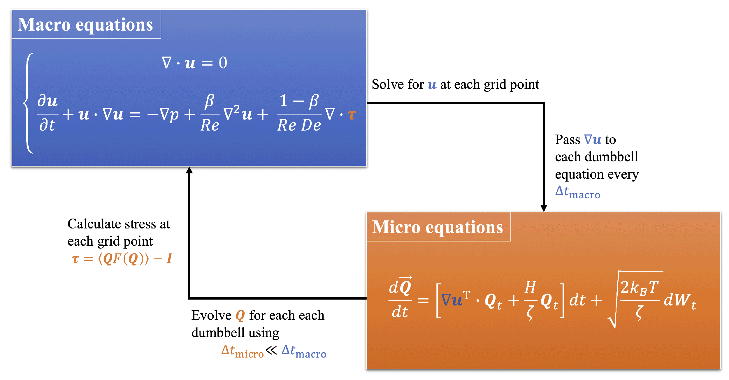
Appendix A.1. Flow Diagram

Figure A1 shows a flow diagram describing the procedure followed to couple micro- and macroscale equations.
Figure A1. Coupling of equations at the micro- and macroscales.
Applsci 13 12265 g0a1

Appendix A.2. Computational Resources

Simulations were performed at USC’s Hyperion cluster. The cluster is a heterogeneous configuration, consisting of 291 compute nodes, 8 large memory nodes, 53 GPU nodes, a large SMP system, and 2 IBM Power8 quad GPU servers. All nodes are connected via a high-speed, low latency, InfiniBand network at 100 Gb/s. All nodes are also connected to a 1.4 petabyte high-performance GPFS scratch filesystem and 450 terabytes of home directory storage.
Figure A2 shows a comparison of running time between parallel and serial computations for simple shear flow.
Figure A2. Wall clock time comparison for viscometric computations in simple shear flow for Hookean dumbbells. Speedup using GPU increases with the number of dumbbells considered.
Applsci 13 12265 g0a2

Appendix A.3. Capillary Thinning Results Using FENE-P Model

In this section, we compare the results shown in Figure 10 for the FENE dumbbell model with those obtained using a macroscopic closure, namely a FENE-P model. The predictions of the FNE-P model are given in Figure A3.
Figure A3. Principal stress difference obtained from simulations of the FENE-P model. These results are comparable to those shown in Figure 10. The differences arise because the FENE-P model is not an exact closure for the FENE dumbbell model and some information is lost by the approximation used in the FENE-P model.
Applsci 13 12265 g0a3

References

  1. Hutchings, I.; Tuladhar, T.; Mackley, M.; Vadillo, D.; Hoath, S.; Martin, G. Links between ink rheology, drop-on-demand jet formation, and printability. J. Imaging Sci. Technol. 2009, 53, 1–8. [Google Scholar] [CrossRef]
  2. Krishnan, J.; Deshpande, A.; Kumar, P. Rheology of Complex Fluids; Springer: New York, NY, USA, 2010. [Google Scholar]
  3. Ulery, B.; Nair, L.; Laurencin, C. Biomedical applications of biodegradable polymers. J. Polym. Sci. Part Polym. Phys. 2011, 49, 832–864. [Google Scholar] [CrossRef] [PubMed]
  4. Barbati, A.; Desroches, J.; Robisson, A.; McKinley, G. Complex fluids and hydraulic fracturing. Annu. Rev. Chem. Biomol. Eng. 2016, 7, 415–453. [Google Scholar] [CrossRef] [PubMed]
  5. Guo, Y.; Patanwala, H.; Bognet, B.; Ma, A. Inkjet and inkjet-based 3D printing: Connecting fluid properties and printing performance. Rapid Prototyp. J. 2017, 23, 562–576. [Google Scholar] [CrossRef]
  6. Ewoldt, R.; Saengow, C. Designing complex fluids. Annu. Rev. Fluid Mech. 2022, 54, 413–441. [Google Scholar] [CrossRef]
  7. Reith, D.; Mirny, L.; Virnau, P. GPU Based Molecular Dynamics Simulations of Polymer Rings in Concentrated Solution: Structure and Scaling. Prog. Theor. Phys. Suppl. 2011, 191, 135–145. [Google Scholar] [CrossRef]
  8. José dos Santos Brito, C.; Vieira-e-Silva, A.L.B.; Almeida, M.W.S.; Teichrieb, V.; Marcelo Xavier Natario Teixeira, J. Large Viscoelastic Fluid Simulation on GPU. In Proceedings of the 2017 16th Brazilian Symposium on Computer Games and Digital Entertainment (SBGames), Curitiba, Brazil, 2–4 November 2017; pp. 134–143. [Google Scholar] [CrossRef]
  9. Ingelsten, S.; Mark, A.; Jareteg, K.; Kádár, R.; Edelvik, F. Computationally Efficient Viscoelastic Flow Simulation Using a Lagrangian-Eulerian Method and GPU-acceleration. J. Non-Newton. Fluid Mech. 2020, 279, 104264. [Google Scholar] [CrossRef]
  10. Yang, K.; Su, J.; Guo, H. GPU accelerated numerical simulations of viscoelastic phase separation model. J. Comput. Chem. 2012, 33, 1564–1571. [Google Scholar] [CrossRef]
  11. Bergamasco, L.; Izquierdo, S.; Ammar, A. Direct numerical simulation of complex viscoelastic flows via fast lattice-Boltzmann solution of the Fokker–Planck equation. J. Non-Newton. Fluid Mech. 2013, 201, 29–38. [Google Scholar] [CrossRef]
  12. Gutierrez-Castillo, P.; Kagel, A.; Thomases, B. Three-dimensional viscoelastic instabilities in a four-roll mill geometry at the Stokes limit. Phys. Fluids 2020, 32, 023102. [Google Scholar] [CrossRef]
  13. Schram, R.; Barkema, G. Simulation of ring polymer melts with GPU acceleration. J. Comput. Phys. 2018, 363, 128–139. [Google Scholar] [CrossRef]
  14. Behbahani, A.; Schneider, L.; Rissanou, A.; Chazirakis, A.; Bacova, P.; Jana, P.; Li, W.; Doxastakis, M.; Polinska, P.; Burkhart, C. Others Dynamics and rheology of polymer melts via hierarchical atomistic, coarse-grained, and slip-spring simulations. Macromolecules 2021, 54, 2740–2762. [Google Scholar] [CrossRef]
  15. Bird, R.B.; Curtiss, C.F.; Armstrong, R.C.; Hassager, O. Dynamics of Polymeric Liquids, Volume 2: Kinetic Theory; Wiley: Hoboken, NJ, USA, 1987. [Google Scholar]
  16. Alves, M.; Oliveira, P.; Pinho, F. Numerical Methods for Viscoelastic Fluid Flows. Annu. Rev. Fluid Mech. 2021, 53, 509–541. [Google Scholar] [CrossRef]
  17. Cruz, C.; Chinesta, F.; Régnier, G. Review on the Brownian Dynamics Simulation of Bead-Rod-Spring Models Encountered in Computational Rheology. Arch. Comput. Methods Eng. 2012, 19, 227–259. [Google Scholar] [CrossRef]
  18. Keunings, R. Micro-Macro Methods for the Multiscale Simulation of Viscoelastic Flow Using Molecular Models of Kinetic Theory. Rheol. Rev. 2004, 2004, 67–98. [Google Scholar]
  19. Owens, R.G.; Phillips, T.N. Computational Rheology; World Scientific: Singapore, 2002. [Google Scholar]
  20. Walters, K.; Webster, M.F. The Distinctive CFD Challenges of Computational Rheology. Int. J. Numer. Methods Fluids 2003, 43, 577–596. [Google Scholar] [CrossRef]
  21. Feigl, K.; Laso, M.; Oettinger, H.C. CONNFFESSIT approach for solving a two-dimensional viscoelastic fluid problem. Macromolecules 1995, 28, 3261–3274. [Google Scholar] [CrossRef]
  22. Halin, P.; Lielens, G.; Keunings, R.; Legat, V. The Lagrangian Particle Method for Macroscopic and Micro–Macro Viscoelastic Flow Computations. J. Non-Newton. Fluid Mech. 1998, 79, 387–403. [Google Scholar] [CrossRef]
  23. Le Bris, C.; Lelievre, T. Micro-macro models for viscoelastic fluids: Modelling, mathematics and numerics. Sci. China Math. 2012, 55, 353–384. [Google Scholar] [CrossRef]
  24. Lozinski, A.; Owens, R.G.; Phillips, T.N. The Langevin and Fokker–Planck Equations in Polymer Rheology. In Handbook of Numerical Analysis; Elsevier: Amsterdam, The Netherlands, 2011; Volume 16, pp. 211–303. [Google Scholar] [CrossRef]
  25. Xu, X.; Yu, P. A multiscale SPH method for simulating transient viscoelastic flows using bead-spring chain model. J. Non-Newton. Fluid Mech. 2016, 229, 27–42. [Google Scholar] [CrossRef]
  26. Bhave, A.V.; Armstrong, R.C.; Brown, R.A. Kinetic theory and rheology of dilute, nonhomogeneous polymer solutions. J. Chem. Phys. 1991, 95, 2988–3000. [Google Scholar] [CrossRef]
  27. Herrchen, M.; Öttinger, H.C. A detailed comparison of various FENE dumbbell models. J. Non-Newton. Fluid Mech. 1997, 68, 17–42. [Google Scholar] [CrossRef]
  28. Chase, D.; Cromer, M. Roles of chain stretch and concentration in capillary thinning of polymer solutions. Fluid Dyn. Res. 2023; in revision. [Google Scholar]
  29. Öttinger, H.C. Stochastic Processes in Polymeric Fluids: Tools and Examples for Developing Simulation Algorithms; Springer Science & Business Media: Berlin/Heidelberg, Germany, 2012. [Google Scholar]
  30. Öttinger, H.C.; Van Den Brule, B.; Hulsen, M. Brownian configuration fields and variance reduced CONNFFESSIT. J. Non-Newton. Fluid Mech. 1997, 70, 255–261. [Google Scholar] [CrossRef]
  31. Jourdain, B.; Le Bris, C.; Lelièvre, T. On a variance reduction technique for micro–macro simulations of polymeric fluids. J. Non-Newton. Fluid Mech. 2004, 122, 91–106. [Google Scholar] [CrossRef]
  32. Bonvin, J.; Picasso, M. Variance reduction methods for CONNFFESSIT-like simulations. J. Non-Newton. Fluid Mech. 1999, 84, 191–215. [Google Scholar] [CrossRef]
  33. Bertola, V. Dynamic wetting of dilute polymer solutions: The case of impacting droplets. Adv. Colloid Interface Sci. 2013, 193, 1–11. [Google Scholar] [CrossRef] [PubMed]
  34. Ardekani, A.; Sharma, V.; McKinley, G. Dynamics of bead formation, filament thinning and breakup in weakly viscoelastic jets. J. Fluid Mech. 2010, 665, 46–56. [Google Scholar] [CrossRef]
  35. Prieto, J.L.; Bermejo, R.; Laso, M. A semi-Lagrangian micro–macro method for viscoelastic flow calculations. J. Non-Newton. Fluid Mech. 2010, 165, 120–135. [Google Scholar] [CrossRef]
  36. Lee, E.C.; Solomon, M.J.; Muller, S.J. Molecular orientation and deformation of polymer solutions under shear: A flow light scattering study. Macromolecules 1997, 30, 7313–7321. [Google Scholar] [CrossRef]
  37. Ghosh, I.; McKinley, G.H.; Brown, R.A.; Armstrong, R.C. Deficiencies of FENE dumbbell models in describing the rapid stretching of dilute polymer solutions. J. Rheol. 2001, 45, 721–758. [Google Scholar] [CrossRef]
  38. Li, J.; Fontelos, M.A. Drop dynamics on the beads-on-string structure for viscoelastic jets: A numerical study. Phys. Fluids 2003, 15, 922–937. [Google Scholar] [CrossRef]
  39. Clasen, C.; Eggers, J.; Fontelos, M.A.; Li, J.; McKinley, G.H. The beads-on-string structure of viscoelastic threads. J. Fluid Mech. 2006, 556, 283–308. [Google Scholar] [CrossRef]
  40. Bhat, P.P.; Appathurai, S.; Harris, M.T.; Pasquali, M.; McKinley, G.H.; Basaran, O.A. Formation of beads-on-a-string structures during break-up of viscoelastic filaments. Nat. Phys. 2010, 6, 625–631. [Google Scholar] [CrossRef]
  41. Wagner, C.; Bourouiba, L.; McKinley, G.H. An analytic solution for capillary thinning and breakup of FENE-P fluids. J. Non-Newton. Fluid Mech. 2015, 218, 53–61. [Google Scholar] [CrossRef]
  42. Eggers, J. Nonlinear dynamics and breakup of free-surface flows. Rev. Mod. Phys. 1997, 69, 865. [Google Scholar] [CrossRef]
  43. Forest, M.G.; Wang, Q. Change-of-type behavior in viscoelastic slender jet models. Theor. Comput. Fluid Dyn. 1990, 2, 1–25. [Google Scholar] [CrossRef]
  44. Guzel, A.; Layton, W. Time filters increase accuracy of the fully implicit method. BIT Numer. Math. 2018, 58, 301–315. [Google Scholar] [CrossRef]
  45. Middleman, S. Stability of a viscoelastic jet. Chem. Eng. Sci. 1965, 20, 1037–1040. [Google Scholar] [CrossRef]
  46. Goldin, M.; Yerushalmi, J.; Pfeffer, R.; Shinnar, R. Breakup of a laminar capillary jet of a viscoelastic fluid. J. Fluid Mech. 1969, 38, 689–711. [Google Scholar] [CrossRef]
  47. Brenn, G.; Liu, Z.; Durst, F. Linear analysis of the temporal instability of axisymmetrical non-Newtonian liquid jets. Int. J. Multiph. Flow 2000, 26, 1621–1644. [Google Scholar] [CrossRef]
Figure 1. Dumbbell configuration given by the coordinates of each dumbbell, r 1 and r 2 , or its center of mass, r c and end-to-end vector, Q .
Applsci 13 12265 g001
Figure 2. Extra stress results in viscometric simple shear flow for Hookean dumbbells (Equation (11)) and UCM model (Equation (17)). The first normal stress difference is calculated as N 1 = τ y y τ x x . All variables are non-dimensionalized using the scaling given in Equation (3) and parameter values given in Table 1.
Applsci 13 12265 g002
Figure 3. Extra stress in viscometric simple shear flow for FENE models compared to the FENE-P closure (Equation (24)). All variables are non-dimensionalized using the scaling given in Equation (3) and parameter values given in Table 1.
Applsci 13 12265 g003
Figure 4. Stochastic simulations for the FENE model with different values of the nonlinear parameter b. All variables are non-dimensionalized using the scaling given in Equation (3) and parameter values given in Table 1.
Applsci 13 12265 g004
Figure 5. Scatter plots of Q x and Q y in simple shear flow for two values of the Deborah number D e . Note: the scale of the scatter plots is not the same across the different plots.
Applsci 13 12265 g005
Figure 6. Probability distribution function (PDF) of dumbbells’ orientation as a function of time and Deborah number ( D e ).
Applsci 13 12265 g006
Figure 7. Expansion ratio as a function of time and Deborah number. The ratio is calculated using Equation (32).
Applsci 13 12265 g007
Figure 8. Axes of extension as a function of time and D e = 500 . Distribution plots at the bottom have been normalized by their corresponding maximum values. Between 0 and 100, the system is in the linear regime, and the stretching in the x- and y-directions are proportional to each other. In the nonlinear regime, t > 100 , the molecules stretch more in the direction of the flow field, i.e., the x-direction. As the stretching approaches the maximum dumbbell length ( b = 300 ), the stretching is ’accumulated’ at the end of the spectrum.
Applsci 13 12265 g008
Figure 9. Comparison of FENE-P model (Equation (24)) with stochastic simulations (Equation (13)) under viscometric elongational flow.
Applsci 13 12265 g009
Figure 10. Filament stretching evolution coupled with microstructure evolution. In this model, the microstructure is represented by non-interacting dumbbells, and their conformation is given by the expansion ratio in Equation (32). Other parameters are β = 0.27 , O h = 0.04 , k = 0.8 , and b = 10 5 .
Applsci 13 12265 g010
Figure 11. Filament and microstructure evolution for different wavelength numbers. Other parameters are β = 0.27 , O h = 0.04 , D e = 0.8 , and b = 10 5 .
Applsci 13 12265 g011
Figure 12. Effects of different FENE parameter. Other parameters are β = 0.27 , O h = 0.04 , k = 0.8 , and D e = 0.8 .
Applsci 13 12265 g012
Disclaimer/Publisher’s Note: The statements, opinions and data contained in all publications are solely those of the individual author(s) and contributor(s) and not of MDPI and/or the editor(s). MDPI and/or the editor(s) disclaim responsibility for any injury to people or property resulting from any ideas, methods, instructions or products referred to in the content.

