Article

A Decision Support System Based on the Integration of a Theory of Constraints and Strategic Management Tools for the Selection of Product Mixes

1
Institute for Transport Planning and Logistics, Hamburg University of Technology, 21071 Hamburg, Germany
2
Department of Industrial Engineering, Faculty of Engineering, Cukurova University, Sarıçam, 01250 Adana, Türkiye
*
Author to whom correspondence should be addressed.
Appl. Sci. 2023, 13(22), 12191; https://doi.org/10.3390/app132212191
Submission received: 2 October 2023 / Revised: 27 October 2023 / Accepted: 6 November 2023 / Published: 9 November 2023
(This article belongs to the Section Applied Industrial Technologies)

Abstract

:
The selection of products to be offered on the market is a critical decision-making process encountered in all industry sectors. It is not just a matter of maximizing profit or optimizing the utilization of corporate resources but also specifically concerns determining a product portfolio that is most suitably aligned to corporate strengths and that appeals to the most attractive and emerging markets. Hence, corporate competencies such as strategic management and production capabilities must be taken into account concurrently. Starting from this point of view, a twofold decision support system (DSS) has been developed. On the one hand, a theory of constraints (TOC)-based analytic hierarchy process (AHP) approach, including a taboo search algorithm, has been developed in order to derive the right product mix for maximizing the total profit amount by considering the bottleneck problem. On the other hand, a GE/McKinsey screen matrix is added to this consolidated approach to support decision-makers in the formulation of product portfolio strategies. The DSS provides a platform to compare outputs coming from the preceding two processes, which allows for the refinement of the solution. The proposed DSS is executed with a problem dataset from the industry to test its accuracy and reliability.

1. Introduction

As Komijan et al. [1] point out, the “product mix problem (PMP) is one of the most complicated problems in production systems”. Solution approaches employing the TOC have gained great momentum since the early 1990s. Goldratt improved the concept of the TOC by incorporating the notion of an effective management philosophy on improvement, based on a five-step heuristic to increase the product throughput of a production system [2]:
  • Identify the constraints.
  • Decide how to exploit the constraints.
  • Subordinate everything else to the above decision.
  • Elevate the constraints.
  • If, in the previous steps, a constraint has been broken, go back to step 1. Do not let inertia become the constraint.
Only the first two of the five steps are applied to derive the product-mix solution. Researchers have already dealt with the solution of PMP under TOC conditions in many aspects [3,4,5,6,7]. According to Wu et al. [8], the TOC has had a significant influence on productivity enhancement in industrial systems.
The most traditional method for selecting the product mix employs the margin heuristic, where those products having the highest individual product margins with higher priority are selected, regardless of the time spent on bottlenecks [5]. The TOC-derived heuristic, however, proposes that product lines should be selected according to their ratio of throughput per time spent on system constraints [2,9,10,11,12,13].
The situation, however, is more complex than it seems. The challenges faced are categorized by the multitude of bottlenecks, the dominance rule adopted in the sequencing of products, and production over integer quantities. If demand exceeds the capacity of the production system, more than one bottleneck may exist. Although it is argued that TOC-derived heuristics are successful in single-bottleneck environments [6,13,14,15,16], Linhares [17] demonstrated that a TOC-derived heuristic may not lead to the optimal solution, even in single-bottleneck environments. Some of the researchers focused on multi-bottleneck systems [4,5,6,7,9,10,11,12,13,14,15,16,17,18]. However, algorithms developed to solve PMP have failed in multi-bottleneck environments since all decisions are made based on the most capacitated constraint, namely, the dominant bottleneck. In determining a product mix, previous researchers merely used the priorities assigned to products by the dominant bottleneck. Considering only one bottleneck in decision-making and ignoring the importance of other ones may distort the solution because only part of the information is used [1]. The initial TOC-based traditional algorithms were presented by Luebbe and Finch [6] and Patterson [13]. They asserted that TOC-derived heuristics could lead to an optimal solution via an integer linear programming (ILP) model. This assertion was also supported by Plenert [7], Maday [19], and Posnack [20]. Although PMP can be formulated as an ILP model, as the number of products increases, the difficulty of solving the ILP model increases exponentially [1].
Following these developments, a series of approaches were propounded, such as the revised algorithm [4], dominance rule-based algorithm [21], and advanced heuristics such as genetic algorithms [22,23] and the tabu-search (TS) [24], providing new policies to deal with the combinatorial complexity of PMP with multiple constrained resources. The revised algorithm tries to improve the solution using an iterative decrease and increase process. Aryanezhad and Komijan [18] discussed several disadvantages of the revised algorithm and the stopping condition of the revised algorithm, stating that it was not defined properly as it might cause the algorithm to reach a non-optimum solution. They then developed their own algorithm, called the “improved algorithm”, which is equipped with a neighborhood search process involving firm stopping conditions.
The literature on methods for solving problems with a multi-bottleneck is rapidly growing. Bhattacharya et al. [25] modeled the problem using fuzzy linear programming. Mishra et al. [26] proposed a TS and simulated annealing hybrid approach. Singh et al. [27] proposed an approach based on Maslow’s need hierarchy theory. Wang et al. [28] also used immune-based approaches, such as self-adaptive regulation and vaccination. Recently, Ray et al. [29] presented an integrated heuristic model comprising the AHP and the TOC (AHP-TOC heuristic) in a decision model, in which the priority of a product and a resource center optimize the product throughput in a multiple-constraint resource environment. Wang et al. [30] reviewed the AHP-TOC heuristic and illustrated its shortcomings.
In this overview of PMP literature, we can conclude that although the optimum product mix may sometimes include products with the lowest product margin and the lowest ratio of throughput per constraint time, violating the TOC-derived heuristic principle [17], TOC-based heuristic approaches provide efficient solutions (sometimes with some slight modifications) for a wide range of PMP instances within reasonable computation times.
PMP, thus far, has been dealt with principally from the perspective of production, but it must be emphasized that the competitive positions of products in the market play a significant role in the determination of strategic product mixes. Blackstone [9] asserts that companies tend to view products as either “dogs” (which have low profit margins), or as “stars” (with large margins), in line with traditional product margin approaches. To compete in the marketplace, companies, on the one hand, expand and differentiate their product mix in a way that can lead to increased revenues, and, on the other hand, the strategy that they adopt should allow for the optimal utilization of enterprise resources and for obtaining a product mix that maximizes operating profit [31]. Companies are, thus, obliged to determine how to offer the right product mix to the market. Such decisions on optimal product mix are closely associated with the general wisdom suggested by the Boston Consulting Group (BCG) (an introduction is available at www.bcg.com/publications/1970/strategy-the-product-portfolio.aspx (accessed on 2 December 2020)) and their notion of product portfolio strategy [32]. In the formulation of product portfolio strategies, it is essential to gather and aggregate the views of senior executives in a systematic manner.
In this study, the GE-McKinsey matrix (an introduction is available at www.mckinsey.com/business-functions/strategy-and-corporate-finance/our-insights/enduring-ideas-the-ge-and-mckinsey-nine-box-matrix (accessed on 2 December 2020)) is used to decide on a product portfolio strategy, instead of using the BCG method. According to Kieltyka et al. [33], a McKinsey matrix has these strengths: (i) it helps to prioritize limited resources in order to maximize return, (ii) managers have a better understanding of how their goods or business divisions operate, and (iii) it will determine the strategic initiatives that the organization should take to improve the performance of its business portfolio. GE has many advantages over BCG since it evaluates the products according to the attractiveness of the market involved and the strength of the firm’s position in the market, with 5 main criteria, including 73 sub-criteria. Moreover, GE consists of nine decision cells with three types of classification (strong, average, weak) instead of four cells with two types of classification (high, low), as in the BCG matrix. There have been studies in the literature concerning the GE matrix as a product portfolio tool. Jang et al. [34] used a GE/McKinsey matrix to measure the attraction of the 15 frontier green construction products and to compare their competencies in terms of strength. In another study, Zihare and Blumberga [35] investigated the market opportunities for cellulose products from combined renewable resources; they made decisions on only two products with potential in the market among a choice of seven products by using GE/McKinsey matrix, which they named “a great tool for decision-making”. Al-Sharrah et al. [36] used the GE/McKinsey matrix as a strategic tool to reach their final decision for planning a balanced petrochemical network with acceptable risk after applying the optimization model in relation to a mixed-integer model of the petrochemical industry.
According to Olhager and Wikner [37], to stay competitive in a global market, it is important to identify strategic, tactical, and operational issues by considering the link among markets, products, and production. While Skinner [38] discussed the effect of manufacturing managers’ ignorant behavior on corporate strategy and proposed a systematic model for top managers, Moore [39] emphasized the alignment of marketing and manufacturing strategies and mentioned the existence of several exceptional publications regarding the development of a manufacturing strategy integrated with marketing and overall business strategies. According to Baki and Cheng [40], product-mix optimization is one of the most important factors related to production planning. They proposed a study to define the current process in a production line and to formulate a linear programming model for product-mix optimization. Jaegler et al. [41] presented a study that considers key questions regarding production control system implementation in a high product-mix and/or high routing-mix environment. Chanda et al. [42] proposed a study that deals with the application of linear programming to product mix. According to de Jesus Pacheco [43], the operations plan must be integrated with corporate and business strategies in order to change and adhere to them. However, in the last decade, the number of studies in the literature regarding the development of manufacturing strategy integrating company business strategy and marketing strategy has been increasing, and the topic is becoming more popular. Due to the forces of legal and environmental factors, even though these studies mostly focused on research areas such as sustainability, green manufacturing, and lean manufacturing, addressing these issues will soon be unavoidable for all manufacturing companies, including traditional ones. Dombrowski et al. [44] presented an approach for the development of a manufacturing strategy that was integrated with corporate strategy. Their research allows a unique strategic position that improves competitiveness through specific resources and capabilities in manufacturing, coordinating other functional strategies with corporate strategy after analyzing the internal, external, and competitive position of the company. Other studies have emphasized this subject and elaborated on it in discussions [45,46,47,48,49,50,51,52].
In the present work, we propose a DSS that derives the right product mix with a priority sequence and, in the meantime, offers norm strategies to facilitate the formulation process of a product portfolio. The priority sequence incorporates the product rankings of AHP-TOC heuristics, optimizing the product mix in multi-bottleneck environments. The product portfolio norm strategies are derived from the views of senior executives, as ascertained through a questionnaire. This evaluation technique requires knowledge of raw material cost, hourly rate, selling price, demand, processing time, and a questionnaire that will provide information about the company’s competitive strength and market attractiveness. The major originality of our study is that the proposed DSS provides an assessment platform that includes two different results: the first is an optimal product mix using the AHP-TOC heuristic, and the second employs norm strategies for products.
The next sections of this paper attempt to put forward the functioning mechanism and application of the DSS. The second section provides a brief description of the PMP. In the third section, a detailed explanation of the functioning mechanism of the AHP-TOC heuristic is given. Also included in this part is an outline of the infrastructure of the DSS. In the next section, this is verified with a PMP dataset drawn from the industry. The rest of the paper assesses the DSS’s performance and outlines the conclusions.

2. Description of the Product-Mix Problem

Products that have common operations on the same resources contribute to a company’s total profit in direct proportion to the multiplication of their contribution margin and demand. The main objective function conceptualized in this sense aims at the maximization of profit for several product types, where constraints contain the capacity limit of resources and the maximum value for the production amount of a particular product type. A mathematical formulation of the problem is described below:
M a x   z = i = 1 N x i × C M i i = 1 N
i = 1 N t i j × x i     β j j = 1 M
x i D i   a n d   x i Z + i = 1 N
The objective function (1) of the ILP model maximizes the total profit, where xi is the decision variable representing the quantity of the product type i, and CMi denotes the contribution margin of the product type i, which is the gap between the sales price and the raw material cost. Equation (2) ensures that the capacity of the resources is not exceeded, where βj is the capacity limit of resource j in the planning period, and tij is the processing time for one unit of product i in resource j. In Equation (3), market demand Di indicates the bounds for a quantity of product type i, and the production quantity of the product i is an integer and non-negative.

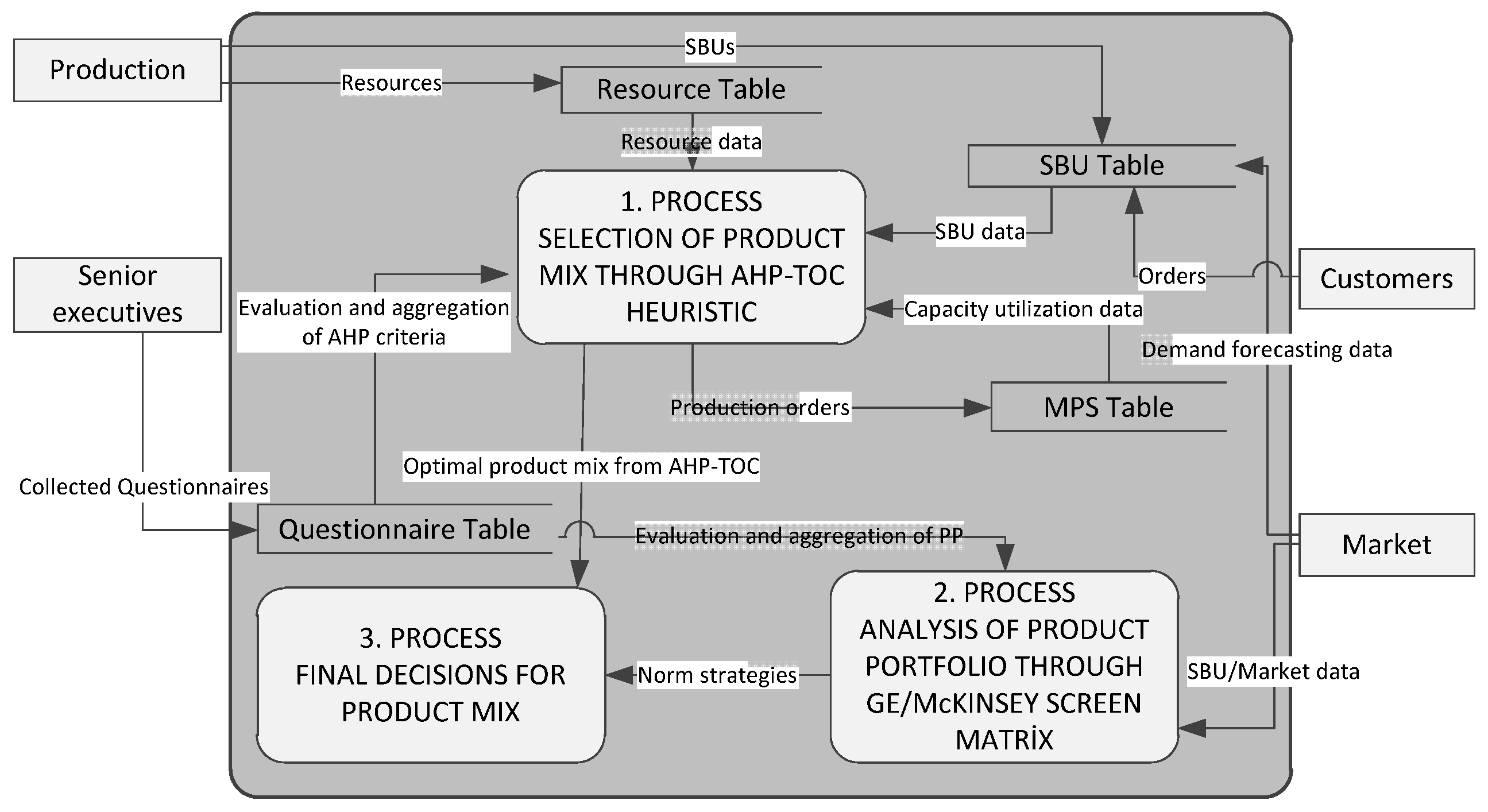
3. System Architecture of the DSS

The optimization-based DSS discussed in this study comprises three key relational components: data management, model management, and dialog management [53]. Model management leverages the AHP-TOC heuristic solution methodology to identify the optimal product mix and conduct the necessary calculations for determining product portfolio norm strategies. Meanwhile, data management involves a relational database for storing datasets and questionnaires.
With its relational structure, data management serves as the primary mechanism for data manipulation. During the execution of the decision support system (DSS), this triad operates as closely interconnected systems. The following section provides detailed explanations of these components of the DSS.

3.1. Data Management

The data management component encompasses a cohesive structure consisting of six principal interconnected tables, including products, sub-products, resources, questionnaires, top management, and production orders.
In the realm of production systems, the prevalent scenario involves a many-to-many relationship between products and sub-products. Notably, industries such as those dealing with metal parts often exhibit a pattern where a final product comprises multiple detailed parts, each of which may be utilized in the assembly of a range of final products. Similar complexities arise in the association between resources and sub-products, stemming from variations in processing time and operation costs across different resources for a single sub-product unit.
The function of production orders within this framework is pivotal, actively contributing to the solution process, particularly in conjunction with the utilization of decision support systems (DSS) alongside ongoing production-planning systems. The computation of the total raw material cost for a specific product involves the aggregation of the raw material costs attributed to the sub-products associated with that product. Similarly, the calculation of the total processing time and processing costs for a product relies on the summation of the corresponding values for the related sub-products across the pertinent resources.
Furthermore, the determination of the contribution margin for a product involves assessing the disparity between its sales price and the total raw material cost. Notably, the designed structure of the database facilitates the incorporation of processing costs into the profit-calculation process. In the context of top management, senior executives, who are responsible for overseeing the strategic business units, provide responses to survey inquiries. Each response is systematically recorded as an entry within the PMP questionnaire table.

3.2. Dialog Management

The dialog management component furnishes users with a graphical user interface that facilitates data entry pertaining to the problem dataset, the execution of the solution procedure, and the display of the resulting solution. Additionally, the survey screen is configured as a web-based platform, ensuring accessibility for remote data processing. It enables functionalities such as data capture from the survey screen, posting to the database, and recording the information in the database system.

3.3. Model Management

The framework of model management is structured around three primary relational processes, as illustrated in Figure 1. The first process is dedicated to the pursuit of an optimal product mix, leveraging the AHP-TOC heuristic algorithm proposed by Ray et al. [29]. The second process entails an in-depth analysis of the product portfolio, facilitated through a questionnaire-based evaluation employing the GE/McKinsey screen matrix. This systematic approach generates a spectrum of norm strategies applicable to the array of products encompassed within the company’s product range. In the context of the BCG matrix, the term “strategic business unit” (SBU) refers to a division within the company, a specific product line within a division, or occasionally an individual product or brand [54]. For the sake of ensuring consistent comprehension, the term SBU is prioritized over “product” in the pertinent sections of this paper.
The final stage serves as a platform for the comparison of outputs derived from the preceding two processes. In the event of coherence within the final product mix, the solution remains fixed; however, if inconsistencies arise, the first and second processes are iteratively executed, incorporating necessary adjustments to the problem data, aligned with norm strategies. Ultimately, this iterative mechanism yields a final product-mix solution.

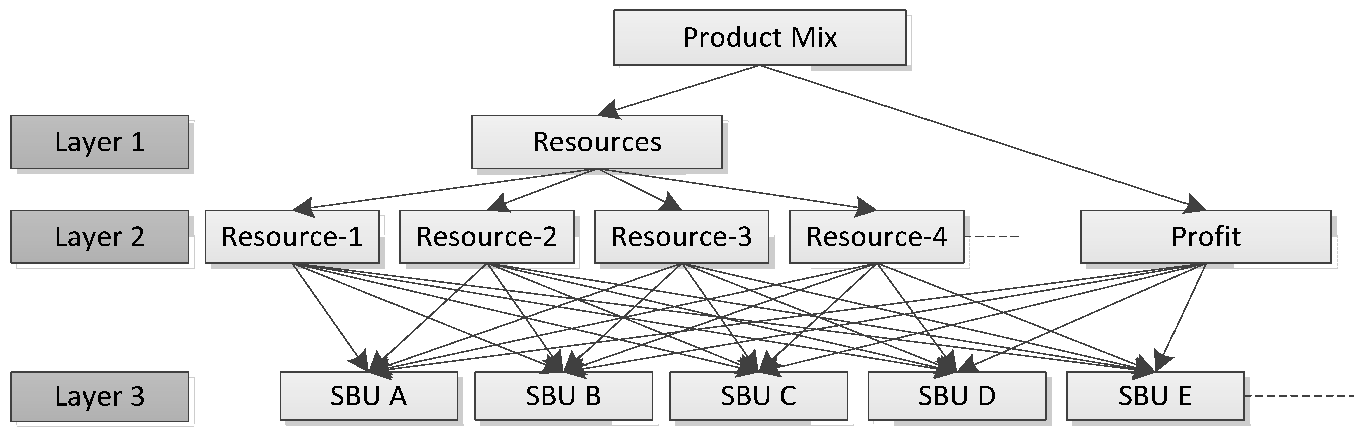
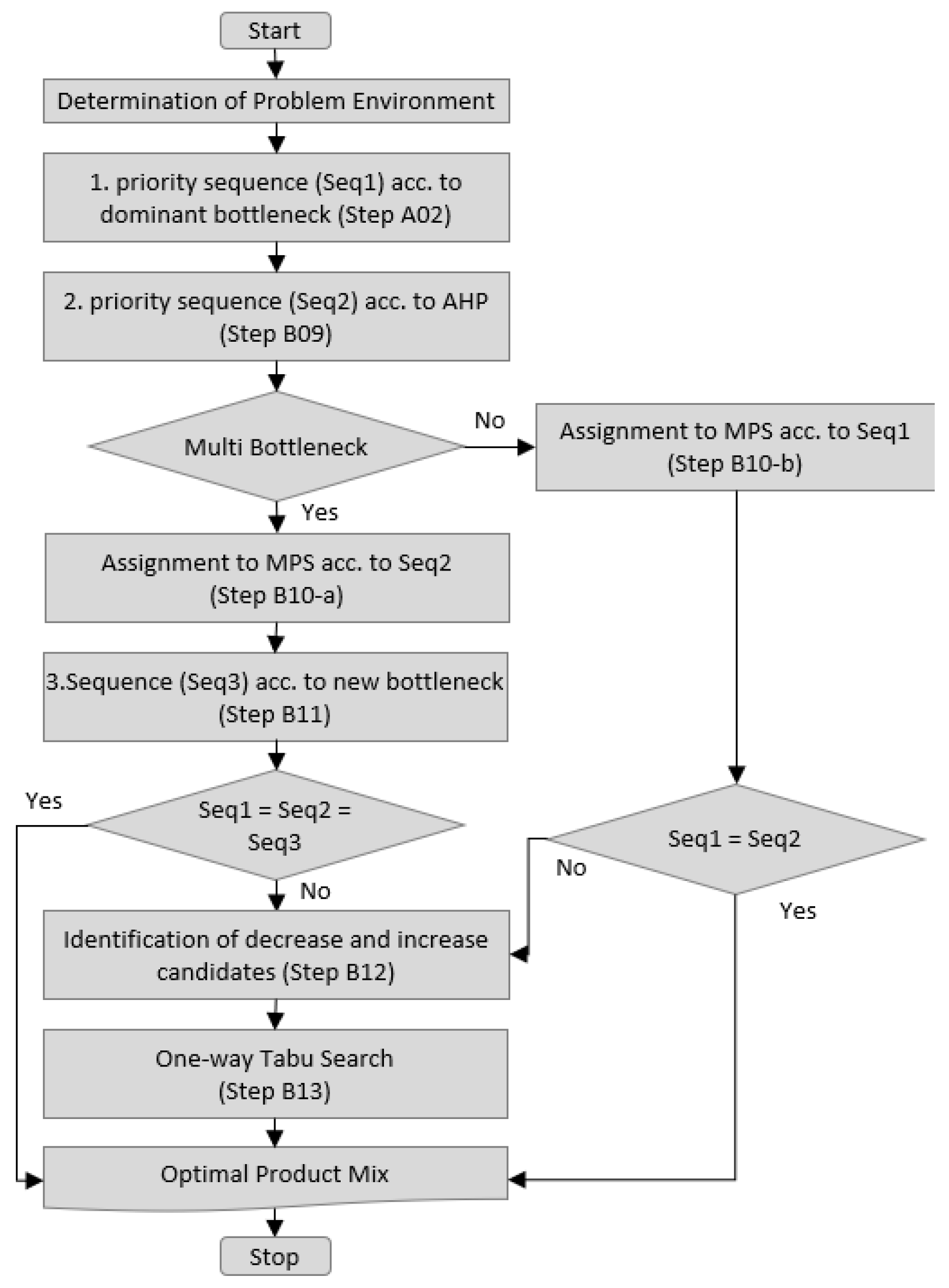
3.3.1. Selection of an Optimal Product Mix under the AHP-TOC Heuristic

The data inputs for the initial process, the AHP-TOC heuristic, are gathered from four distinct tables, specifically, the resource table, SBU tables, the MPS table, and the questionnaire table. These tables aggregate the pertinent data obtained from four external data sources, namely, production, customers, the market, and senior executives. Additionally, an internal data source, the master production schedule (MPS), contributes to the relevant data stored in the MPS table. In the course of executing the AHP-TOC heuristic, the MPS table serves as a repository for production orders and is accessed through ad hoc queries to compute the dynamic capacity utilization data.
Operational information pertinent to production serves as the foundational data, primarily concerning resources such as machinery, workstations, and their respective capacities, as well as SBUs, including the processing time of products across various resources. Customer orders are pivotal for determining the periodic demand attributed to each SBU, considering both historical demand data and proactive demand forecasting endeavors. The actual prices at which the raw materials and final products are being traded in the market are directly associated with the company’s raw materials cost and sales price.
A salient characteristic of the proposed decision support system (DSS) lies in the integration of the decision-maker’s perspective within the determination of the product mix. The involvement of the decision-maker in the solution process aligns with the initial phase of the second step of the theory of constraints (TOC) concept, specifically addressing the optimization of the system’s constraints. The decision matrix, constructed using Saaty’s nine-point scale (Table 1), facilitates the representation of the decision-maker’s viewpoint regarding profit and resource considerations (refer to Figure 2). The decision matrix further serves as the foundational step in prioritizing the relative importance of the first-level criteria within the AHP.
The priority vector, also known as the relative importance, is computed by normalizing the eigenvector of the decision matrix. As the number of elements in the decision matrix is less than 3, it is not possible to assess the consistency ratio [55]. In our model, the consistency can be determined directly by examining the relative values of the elements.
The AHP-TOC heuristic method is organized within a hierarchical framework of three layers. At the foundation, the initial layer systematically integrates the assessment of both resources and profit. The criteria resources represent the importance of exploiting total production capacity, and the profit stands for the importance of the margin between sales price and raw material costs for the whole demanded quantity. Through a meticulous process of pairwise comparison, decision-makers attribute relative significance to the two vital elements of resources and profit, reflecting their core considerations. The outcome of the first layer is the priority vector of the resources and profit.
The second layer delves into a detailed exploration of the relative importance of each individual resource and each individual SBU’s profit, casting light on their contributions within the decision-making process. The second layer entails preliminary computation to obtain the dimensionless decision matrix for SBUs by normalizing their contribution margins, the normalized matrix of the SBU processing times, and the normalized matrix of the actual time and the available time, as well as the normalized matrix of capacity and processing times.
Finally, the third layer is dedicated to discerning the hierarchies within SBUs and unraveling their interplay. The layer yields a priority sequence for SBUs, computed by multiplying the normalized contribution margin for each SBU by the weighted vector of profit and subsequently adding the order of priority of the resources. This resource priority is determined by the product of the resultant vector of resources and that of the normalized matrix of capacity and processing times obtained from the second layer.
For handling more complex decision-making structures, we propose the implementation of a comprehensive strategy informed by established methodologies. Drawing from the works of Saaty [55] and Vargas [56], our proposition aligns with the “divide and conquer approach” recommended in the literature. This approach involves segmenting the elements into coherent clusters, enabling more focused pairwise comparisons and alleviating the computational burden associated with employing a large number of elements [57]. Additionally, inspired by the principles of continual improvement advocated by Ishizaka and Labib [58], we emphasize the integration of “iterative refinement”, enabling the continual reassessment and adjustment of pairwise comparisons to accommodate the evolving perspectives and insights.
The result, derived from the AHP, yields a provisional product mix, highlighting the necessity for a more refined optimization approach. To that end, we introduced a TS algorithm aimed at identifying optimal product-mix solutions. TS is a metaheuristic search method designed to address complex optimization problems by navigating through a diverse solution space. Introduced by Glover [59] in the 1980s, TS draws inspiration from the concept of memory, incorporating a dynamic mechanism to avoid revisiting previously explored solutions. By employing a strategic memory-based approach, TS effectively balances exploration and exploitation, enabling the efficient exploration of promising solution areas while maintaining the capability to escape local optima. This versatile optimization technique has found applications in various fields, including combinatorial optimization, scheduling, and logistics, demonstrating its robustness and effectiveness in tackling intricate real-world problems.
Concerning the requirements of the AHP-TOC heuristic, the following notations are selected.
i
j
k
q
N
M
Ri
Di
Pi
Product index
Resource index
Demand condition
Number of bottlenecks
Number of products
Number of resources
Raw material cost of product i
Demand for product i
Market price of product i
tij
βj
CMi
RCij
TRCj
dj
 
CR
BN
Processing time of product i on resource j
Total available capacity of resource j
Contribution margin of product i
Utilized capacity of resource j for product i
Total utilized capacity of resource j
Difference between total capacity and required
capacity of resource j
Set of constraint resources
Bottleneck
The AHP-TOC heuristic [29], together with the improvements in identifying the problem environment and decrease-increase procedure, is illustrated in Figure 3 and is applied as follows (this section substantially adopts a similar stepping hierarchy and formulations to the original AHP-TOC heuristics of Ray et al. [29], to distinguish the improvements and provide a structured telling in the section case illustration).
Step A is devoted to the identification of the system’s constraints. A further step, A03, is added to the original approach to enhance the identification of the problem environment, and whether it is a single or multi-bottleneck environment. After that, to create different demand conditions, an artificial variable (L) is added to the formula for utilized capacity (RCij). As a result, a relatively larger coefficient is given in the function to penalize the utilized capacities for a certain product. This specific sub-procedure is demonstrated as follows, where the k (identical to i) of different demand conditions are derived by boosting the demand for a certain product while maintaining the others at the same level within a loop through the products.
If the multi-bottleneck procedure returns a true result (Algorithm 1), then the problem should be regarded as a multi-bottleneck environment. Otherwise, there is a single real bottleneck in the production system.
Algorithm 1: Multi-bottleneck procedure to identify the problem environment. (In the present study, L was initialized with 10).
Procedure Multi-Bottleneck:boolean
  input L, dj, RCij, TRCj, Seqk
  for k = 1…N
       if i = k
       RCij = tij × Di × L
       else
       RCij = tij × Di
       endif
       TRCj = i N R C i j
       dj = βj − TRCj
       Seqk = Rank(dj)
  for k = 1…N − 1
       for i = k + 1…N
        If SeqkSeqi
          return true
          break
        endif
Step B involves exploiting the system’s constraints. The procedures, from the determination of the decision matrix and the calculation of the priority vector of the resource and profit to the normalization of contribution margin, processing times, and the required time or maximum available time (steps B01 to B07), are the same as those given by Ray et al. [29].
Step B08: Determine the decision matrix (fi) by multiplying the matrices of the normalized processing times and the normalized required time or the maximum available times obtained, respectively, in Steps B05 and B07. Unlike the procedure of Ray et al. [29], the reciprocal of the decision matrix (hi) is considered as follows.
p 11 p 1 m p n 1 p n m × q 1 . . q m = f i . . f n
h i = 1 f i i = 1 N 1 f i , i = 1 N
Step B09: Obtain a priority sequence (Wi) for the products by summing up the multiplication of the normalized dimensionless decision matrix (ri) by the weighted vector of profit (Step B02) and the multiplication of the reciprocal of the decision matrix (hi) by the weighted vector of resources (Step B02). Finally, if the type of problem environment is characterized as a multi-bottleneck, then, we proceed to Step B10-a. Otherwise, we move to Step B10-b.
Step B10-a: Allocate products to the MPS according to the priority sequence from Step B09 until it schedules the largest feasible quantity without exceeding demand and resource capacity. When the capacity of any constraint resource is used up or if the remaining capacity is not enough to produce another unit of product, then, a feasible MPS is achieved. The stopping condition regarding the allocation to MPS refers to the point when the capacity of every CR is used up or when there are no products remaining to be allocated to the CRs. Finally, we proceed to Step B11.
Step B10-b: Using the same rules given in Step B10-a, we allocate products to the initial MPS, according to the priority sequence from Step A02. If the priority sequences obtained in Steps A02 and B09 are identical, then, we deliver the optimal product mix. Otherwise, we proceed to Step B12.
Step B11: Determine the new bottleneck. Then, by calculating the profit-per-unit constraint time of all the products on the new bottleneck, a new priority sequence is obtained. Finally, we compare the resulting priority sequence with the one already obtained in Steps A02 and B09. If these sequences are identical, then, allocate products to MPS accordingly and deliver the optimal product mix. Otherwise, proceed to Step B12.
Step B12: Identify the candidate products for the loops of decrease (P) and increase (Q). For this purpose, we first compare the priority sequences of B09 and B11. To be able to identify the Ps and Qs, the following conditions must be provided:
(1)
In the first priority sequence, P is prior to Q.
(2)
Product Q should meet three conditions:
(a)
Its demand is not fully met;
(b)
It is prior to P in the second priority sequence;
(c)
In the second priority sequence that it is prior to P, it is prior to all the products where their demands have not been fully met.
(3)
The Q candidates are sorted in descending order in the second priority sequence.
Step B13: In this step, a TS algorithm is employed, whereby the possibility is explored if the one-unit change in the quantity of a product leads to a better total profit, provided that the limited capacity of the bottlenecks is not exceeded. Apart from a classical TS, neighboring moves take place among predetermined decrease candidates. In this direction, we reduce one unit of P and increase Q until one of the following stopping conditions is achieved [18]:
(1)
The demand of Q is fully met.
(2)
It is not possible to increase Q due to the lack of capacity. If the demand of a superior Q candidate is met or if it is not possible to increase it further, we proceed with the next Q and repeat this procedure with all Q candidates. We reiterate this procedure until it is not possible to increase Q. If there is more than one P, we run the following procedure (Algorithm 2):
Algorithm 2: One-way tabu search procedure.
procedure One-way-TS
  input: n (number of P candidates), φ (arbitrary parameter for maximum units to decrease), α (aspiration level), δ (diversification level), τ (tabu list size).
  Declare variables, S (a subset of neighbouring moves) and T (product-mix solution)
  for i = 1,, φ
  for S ← neighbourhoodSpace(i) = 1,, (i + 2)n (i + 1)n
     if isTabu(S, α, δ)
       continue
     if increaseQ(S)
       Ti = calculateProfit(S)
       If Ts ≥ Tbest
          saveResult(Ts)
       else
          addtoTabulist(S, τ)
  return Tmax
Containing all the possible decrease subsets of the P candidates, the neighborhood space can deterministically be generated as a matrix of size:
(φ + 1)n − 1 × n
The subsets are sorted in a similar way to that seen in a binary search. Each neighboring move goes first through the subroutine isTabu and is then checked over the tabu list. The parameters of aspiration and diversification are preconditions used to execute the subroutine isTabu. If it is a tabu, the neighborhood space is first refined and is then skipped to the next iteration. Otherwise, the subroutine IncreaseQ takes the move as an input parameter and provides a set of permissible increasing quantities, j, according to the rules defined at the beginning of step B13. If an increase is applicable, then, profit Ti is calculated. If the profit is greater than or equal to the best saved profit Tbest, then the solution is saved in the result list. Otherwise, the move is added to the tabu list. Should the occasion arise, the tabu list is revised. If an increase is not possible, then it is skipped to the next iteration. The solution with the highest profit in the eventual results table provides the final product mix.

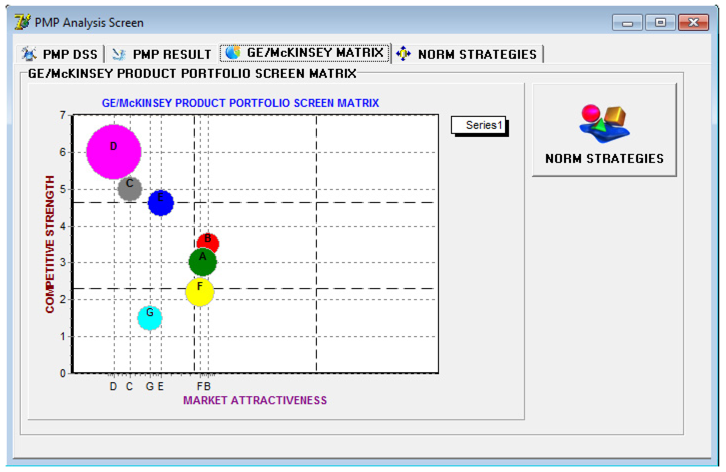
3.3.2. GE/McKinsey Product Portfolio Analysis

The GE/McKinsey product portfolio screen matrix is one of the tools that can be used to help the top management understand the competitive position of SBUs in the market. The competitive position of an SBU is principally characterized by market attractiveness and competitive strength. Market attractiveness is a subjective assessment associated with external factors that are uncontrollable by the company, while competitive strength is a subjective assessment associated with internal factors that are largely controllable by the company [32]. To be able to demonstrate these two dimensions on a common platform, a questionnaire study has generally been accepted as a straightforward approach.
In deriving the survey questions, measures for the axes of the GE/McKinsey screen matrix, market attractiveness, and competitive strength are first considered. Later, the parameters for each measure are determined and consolidated under two dimensions: the main criteria and sub-criteria (see Appendix A). Under the 5 common main criteria, 37 sub-criteria for market attractiveness and 36 sub-criteria for competitive strength are identified.
Within the second process, involving product portfolio analysis, the decision-maker serves as the exclusive authority responsible for evaluating those survey questions aimed at eliciting normative strategies. The initial step involves the allocation of weighting factors by the decision-maker to each main criterion, ensuring that the cumulative sum of the weighting factors equals 100. Decision-makers can, thus, value the corresponding criteria over a seven-point Likert scale. In this way, the answer to a question is parameterized. By multiplying that parameter value by the weighting factor, quantitative measures of product portfolio market attractiveness and the relative competitive strength of the corresponding SBU in that market are obtained.
The functional data inputs to the third process comprise the intermediary outcomes of the preceding processes, the AHP-TOC heuristic, and product portfolio analysis. The AHP-TOC heuristic yields an optimal product mix but does not identify the order of importance. Product portfolio analysis, based on a GE/McKinsey screen matrix, delivers norm strategies (see Appendix B), yielding a range of strategies including invest, harvest/divest, and selective action, as well as the importance order.

3.3.3. Final Solution Procedure for the Product Mix

The final decision process operates in a twofold manner. The first is a scenario where the product mix solution derived by the AHP-TOC heuristic is in compliance with the results garnered from product portfolio analysis; the DSS algorithm results in final strategies for the correct product mix and then terminates. This compliance is characterized by the number of products and production quantity, as well as the importance order.
The other scenario is one where the mentioned compliance is disrupted, on the grounds that the process of product portfolio analysis prescribes a norm strategy that necessitates the elimination of any SBU. In such instances, the DSS algorithm retraces its steps, completely removing the SBUs in question from the product range and isolating pertinent data from the PMP dataset. Subsequently, the algorithm initiates the entire process anew. This iterative cycle persists as long as non-compliance prevails within the final decision process. Ultimately, this iterative mechanism yields non-conflicting sets of product mix and product portfolio strategies.

4. Case Illustration

The present case study considers a PMP dataset, gathered in cooperation with a real company, in order to demonstrate how the whole components of the DSS operate. The relevant information is illustrated in Table 2.
The PMP dataset involves information collected from a yarn manufacturing company, where, in general terms, seven products are manufactured over nine workstations (S1 to S9). The most distinctive characteristic of cotton yarn production is ring stations (S8), where the type of final product is differentiated; all the preceding stations up to this point in the manufacturing process serve to deliver uniform, semi-processed material to S8. For this reason, cotton yarn production can be characterized as a PMP with a single-bottleneck environment [31]. However, the processing times at stations can vary, due to any additional textile raw material used and the time needed for changing the setup between different products.
Steps A01, A02, and A03: Table 2 illustrates the identification of the constraints and the allocation of priority, based on the time difference (dj) between the demanded capacity (TRCj) and resource capacity (βj). Assuming that the total demands for products were allocated to the production schedule, the gap between the available capacities and required capacities determines the dominance level of the constraint resources. The maximum available capacity is calculated in minutes on a monthly basis, over 29 full workdays. The dataset represents a PMP with a multi-bottleneck environment, where CR = (S8, S6, S9).
The adopted approach toward the identification of a multi-bottleneck environment constitutes an underlying problem. The resolution of this problem may be possible by testing the required resources under different demand conditions. If the order of capacity gaps between the required capacity and available capacity according to resources varyies, then the problem should be regarded as a multi-bottleneck environment. Otherwise, there is one real bottleneck in the production system, which possesses the biggest gap in all cases. As was already stated, cotton yarn production is characterized as a PMP with a single-bottleneck environment. This is also substantiated by means of the approach given in Step A03.
Depending on the processing times for bottleneck S8, the SBUs are prioritized again to initiate a new iteration (seq1). The CM-based priority order took shape as A > B > C > E > D > G > F, in consideration of the share of the unit constraint time in the CM (see Table 2).
Steps B01 and B02: Based on Saaty’s nine-point scale, the relative importance of the resources in terms of profit is judged by the decision-maker. The decision matrix for the product mix is, thus, derived. The consistency ratio is employed in order to judge the consistency of the pairwise comparison matrix [55]. In the present case, inconsistency could not occur because n equals only 2.
As can be seen in Table 3, the relative importance of profit is two times more significant compared to the importance of the resource. The relative importance values are computed as average ratios, taking all the collected product surveys into account. The priority vector is calculated via the normalization of the eigenvector derived from the decision matrix.
Steps B03 and B04: Taking the beginning contribution margins of products into consideration, a normalized dimensionless decision matrix (ri) is derived (see Table 4).
Step B05: By dividing each product’s processing time on a resource by the column total of the respective resource, the processing times (pij) under resources are normalized (see Table 4).
Steps B06 and B07: In the same manner, the maximum available capacities of the bottlenecks and the required capacities of slack resources are determined and normalized (qi) (see Table 4).
Step B08: By multiplying the normalized processing times (pij) obtained in Step B05 and the normalized feasible capacities (qj) obtained in Step B07, a reciprocal decision matrix (hi) is derived (see Table 4).
Step B09: A priority sequence for the products is derived by multiplying the normalized contribution margin for each product by the weighted vector of profit (0.667) and then adding the priority of the resources, which is established by the multiplication of the resulting vector of resources (0.333) and the resulting normalized matrix of the capacity and processing times in the preceding step. The new priority sequence, seq2, is lined up as G > A > B > F > E > C > D. This sequence relies on the fact that the relative weight of the contribution margins dominates the priority for products G, F, and E, in contrast to the relative weight of the resources.
Steps B10-a and B10-b: Products are allocated to the initial MPS according to the priority sequence obtained in Step A02 because the PMP has been identified as a single-bottleneck environment (see Table 5). A temporary product mix is formed as 81A, 52B, 57C, 69E, 290D, 51G, and 0F.
This actually implies a branching point, from which the solution procedure can proceed in two directions. The first direction is taken in the situation where the PMP is characterized as a multi-bottleneck environment, followed by Step B11. The second direction relates to the single-bottleneck environment, which subsequently branches out depending on a comparison of the priority sequences from A02 and B09. The second direction is picked up in this case because it relates to a single-bottleneck environment. Due to the discordant priority sequences from A02 and B09, the process continues to step B12.
Step B12: Under the given conditions, the P and Q candidates are set as introduced in Table 6.
Step B13: Considering the product mix from the MPS obtained in Step B10, the loops of neighbouring moves commence. Finally, the profits achieved in the iterations are compared, and the product mix that provides the highest profit is identified as the optimal product mix. After this point, the AHP-TOC heuristic terminates. Step B13 yielded an optimal product mix at the 7th and 11th iteration of the total 31 neighborhood space, where φ = 1, n = 5, α = 0, δ = 0, and τ = 31, as in Table 7.
From this point on, the solution procedure moves on to the GE/McKinsey product portfolio analysis procedure, in order to formulate the product portfolio strategies. By including the scores from the collected questionnaires, the pairs of market attractiveness and competitive strength for each SBU are calculated. The resulting scores are given in Table 8.
From the company where the case study was conducted, three product portfolio questionnaires were collected for each SBU. After the required manipulations of the resulting survey data, the GE/McKinsey matrix took shape, as pictorially illustrated in Figure 4.
Consequently, it can clearly be seen that both the production and marketing strategies of the company in question were in favor of the production of product D because the plant was designed to produce a specific type of product, in accordance with the purpose for which the production plant was established. In addition, the competitive strengths of the company were far more decisive in terms of the formulation of product portfolio strategies, as the market remains quite stable.
Regarding the production of other products, extra setup time and out-of-control non-productive times arise as a result of switching to another product. This is far more obvious in the context of the reduction of yarn fineness than of its thickening. In other words, in contrast to thick yarn, fine yarn is more difficult to manufacture. Due to the production technology and design, senior executives remained more under the influence of the thought that adopting an “invest to grow strategy” would become impossible as long as production diverged from the thickness of the yarn used in product D. This is, in fact, because of the low competitive position of the company, even though the product has great market attractiveness.
As is seen in Figure 5, products D and C fell into the most significant strategy segment, that of “invest to defend a position”. Product E, which has near-thickness with products D and C, follows them, with the strategy of “invest to grow offensively”. For products D and C, the sub-strategies of concentrating the company’s efforts on maintaining strength and seeking dominance against rivals, maximizing investments, and investing at the maximum digestible rate were suggested. There were some drawbacks in production in terms of product E, but still, it is evident that the company had sufficient production capabilities. In the context of producing E, taking action to increase the market share by investment in R&D could be suggested.
Although product B was more favorable than product A in terms of production technology, product A not only had better market attractiveness but also had more demand. Products A and B fell into the average strategy segment in terms of both market attractiveness and competitive strength. Because their relative contribution margins were not high enough, different market segments might be chosen where these products could be sold at better prices. In this direction, selective investments might be made to increase the market share and conduct R&D projects if the product required improvement.
As for product G, there was a quite attractive market for the product, although the company possessed a low level of competitive strength in that market. Product F can be seen as the weakest product, in parallel with the solutions obtained from the AHP-TOC heuristic and the ILP model. The most interesting strategy was one that was suggested for product F. While the market attractiveness was acceptable, a lack of competencies like production technology and workforce would not allow the company to produce this product at the required quality level. This suggests that product F should be divested from the portfolio. If there were a certain demand that must be met or if there were a supply contract that obliged the company to continue its production, the production of obligatory demand would be allowed as a sub-strategy. Otherwise, a divesting strategy that halts the production of the related product should be adopted. In the same manner, stopping all investments in such a product in a sector where investment costs are very high would be the best strategy to adopt.

5. Results and Discussion

With the achievement of the intermediary outcomes of the preceding two processes of the DSS, the AHP-TOC heuristic, and product portfolio analysis, the final decision process could now be performed. In the process of conducting the AHP-TOC heuristic, all demands for products were scheduled to the MPS except for product F and product G, the demand for which was partly covered in the MPS. The obtained product-mix solutions yielded by the AHP-TOC heuristic were also verified through the solution of the ILP model from the CPLEX 300 Solver.
In the process of product portfolio analysis, it was suggested that only product F should be eliminated for quality reasons. In this case, the so-called compliance between the outcomes from the first and second processes is disrupted in terms of the number of products, due to product F. In these circumstances, product F was removed from the product range and the relevant data were isolated from the PMP dataset, meaning that the DSS algorithm went back to the beginning of the AHP-TOC heuristic. The process was started all over again and the same optimal product mix was obtained. Because norm strategies for the rest of the products remained unchanged in the product portfolio analysis, the expected compliance could be found in the final process. Eventually, the DSS results in a non-conflicting product mix through the use of AHP-TOC and a realistic importance order D > C > E > B > A > G > F through product portfolio analysis.
When implementing TOC into the solution of PMP at the first step, the identification of the system’s constraints has always been a controversial issue. To overcome the inefficiencies of the previously developed constraint identification approaches, a specific procedure has been introduced that ensures the discovery of the real dominance order of bottlenecks by taking into account different demand conditions. In addition, directly multiplying the normalized values of processing times and profits, which are multiplied beforehand with their relative weightings, does not make sense. When it comes to the assessment of profit and resources on common ground, a simple transformation is necessary to elicit an effective utilization level of resources and to take it truly into account because these are inversely proportional to each other (for more details, refer to Wang et al. [30]).
The quality of the proposed DSS is essentially associated with the performance of the TS in the last step of the AHP-TOC heuristic. The stopping condition and the superiority order of the candidate products for the decrease procedure, which were previously defined by Ray et al. [29], do not meet the need that arises with the existence of more than one P. For the resolution of this problem, a novel TS procedure is presented in this study, which is based on subsets of the decrease candidates. The proposed procedure, which is based on listing all subsets of the decrease candidates, is efficient for finding the optimal solution in this case. However, the number of decrease subsets mounts up exponentially as the number of decrease candidates (n) and the maximum units to decrease (φ) escalate. This is why it can be concluded that the criteria employed to sort products for the decrease-increase procedure might fail in their task, depending on the problem environment. As Wang et al. [30] pointed out, identifying the Q and P candidates depends principally on whether different product sequences are acquired in any particular step. Depending on the quality of the initial solution, aspiration, intensification, and diversification rules in the TS may be called for. For the reasons outlined above, the efficiency of the proposed concept needs to be elucidated by applying it to different problem sets.
In order to cover up the multi-bottleneck deficiency of the problem dataset, some alterations have been made below, in such a way that the TS also becomes involved. Revising the processing times of products F and G on resource S8 as 0 and 130, respectively, turns the production system into a genuine multi-bottleneck environment. S8 is the first dominant bottleneck, which is the same as previously. After allocation to the MPS in Step B10-a, S6 appears as the new bottleneck. The eventual alignment of sequences to identify the Q and P candidates is given in Table 9.
The TS is provided with the initial solution 81A, 52B, 57C, 268D, 69E, 84F, 63G = 2,255,300. One-way-TS delivers the optimal product mix 81A, 52B, 57C, 290D, 68E, 84F, 53G = 2,260,400 for φ = 10, n = 3, α = 0, δ = 0, and τ = 7.

6. Conclusions

In response to the increased awareness of implementing a manufacturing strategy that is integrated with company strategy, this study proposes a new consolidated model for the selection of product mixes by adding a strategy tool for better product portfolio selection. Considering the fact that corporate competencies, e.g., capacity, quality, technology, and the profit rates of SBU, should all be considered when determining a strategic product mix that both optimizes the utilization of corporate resources and maximizes operating profit, a DSS is proposed in this study. The proposed approach takes into account the priority vectors of profit, resources, and product market as criteria for the determination of a strategic product mix in single- and multi-bottleneck environments. For the resolution of capacity problems, the AHP-TOC heuristic is employed, while the product–market relationship is reflected by the GE/McKinsey product portfolio matrix in accounting for the views of senior executives, which have been extracted by means of a dedicated questionnaire. The most distinctive element of the proposed DSS is that it provides a common platform to assess the optimal product mix under AHP-TOC heuristic conditions, together with the competitive positions of products in the market, by means of the GE/McKinsey screen matrix.
Some weaknesses of the proposed method can be listed as follows:
(1)
The survey answers require that either highly experienced executives or consultants complete the GE/McKinsey product portfolio matrix questionnaire when collecting strategic information.
(2)
The criteria adopted for AHP can be extended with the inclusion of customer requirements. However, the definition of customer requirements can vary, depending on the activity area of the industry.
(3)
Striking the right balance between the combinatorial complexity of PMP and computing capacity is still an indisputable fact that should be considered in the design of a solution procedure.
The advantages of the proposed methodology are the following:
(1)
Both quantitative and qualitative factors are incorporated into the solution process.
(2)
The model is free from impenetrable mathematical expressions. Due to the model’s light computing complexity, the necessary computing time is negligible.
(3)
The model not only delivers an efficient solution but also allows for a readjustment of the product range and refinement of the final product-mix strategies.
(4)
In case of need, the proposed DSS can be adapted easily, with some slight modifications for different time intervals, offering the option to change the product mixes.

Author Contributions

Conceptualization, Y.E., H.O.Y. and E.Y.; methodology, Y.E. and H.O.Y.; software, Y.E.; validation, Y.E., H.O.Y. and E.Y.; formal analysis, Y.E., H.O.Y. and E.Y.; investigation, Y.E.; resources, Y.E.; data curation, Y.E.; writing—original draft preparation, Y.E.; writing—review and editing, H.O.Y. and E.Y.; visualization, Y.E. and H.O.Y.; supervision, H.O.Y.; project administration, none.; funding acquisition, none. All authors have read and agreed to the published version of the manuscript.

Funding

This research received no external funding.

Institutional Review Board Statement

Not applicable.

Informed Consent Statement

Not applicable.

Data Availability Statement

The data presented in this study are available on request from the corresponding author. The data are not publicly available due to privacy.

Conflicts of Interest

The authors declare no conflict of interest.

Appendix A. Main and Sub-Criteria for the Product Portfolio Screen Matrix

Market AttractivenessCompetitive Strength
1. Market
Market dimension
Market growth rate
Average profitability
Market segments/ fragmentation
Price sensitivity
Pricing trends
Demand uncertainty-seasonality of sales
Offer/demand relationship
Energy availability
Global opportunities
Distribution channels
2. Competition
Degree of concentration
Degree of substitution
Sectoral diversity
Product life cycle
Range of product/service
3. Finance and Economics
Profitability
Economy of scale
Entry/Exit barriers
Inflation rate
Exchange rate
Wage levels
Availability of workforce
Sectoral revenue risk
4. Technology and production
Complexity
Differentiation
Patent and copyright
Plants and facilities
Production process
Maturity
Technologic requirements
5. Social and Political
Influx of lobbying
Influx of customer unions
Social attitude and tendency
Role of laws and norms
Influx of fiscal policy
Pollution
1. Market
Business share
Business growth rate
Regional coverage
2. Competition
Business competitiveness
Relative profitability
Relative brand strength
Degree of acceptance
Degree of service
Flexibility for innovation
Ease of access in distribution channels
Management strength
Strength of marketing (CRM)
Strength of human resources
3. Finance and Economics
Return on investment
Added value
Entry/Exit barriers
Ease of buying the raw goods
Cost of human resources
Ease of financing
Relative cost positions
Strength of assets and competencies
Availability of production factors
4. Technology and production
Ease of adaptation to innovations
Degree of specialization/sectoral specialization
Corporate resources/production technology
New product design
Product quality
Production capacity
Productivity
Effectiveness of R&D and innovation
5. Social and Political
Ease of adaptation to changes
Quality of social affairs
Efficiency of promotions
Customer loyalty
Customer focus
Degree of pollution

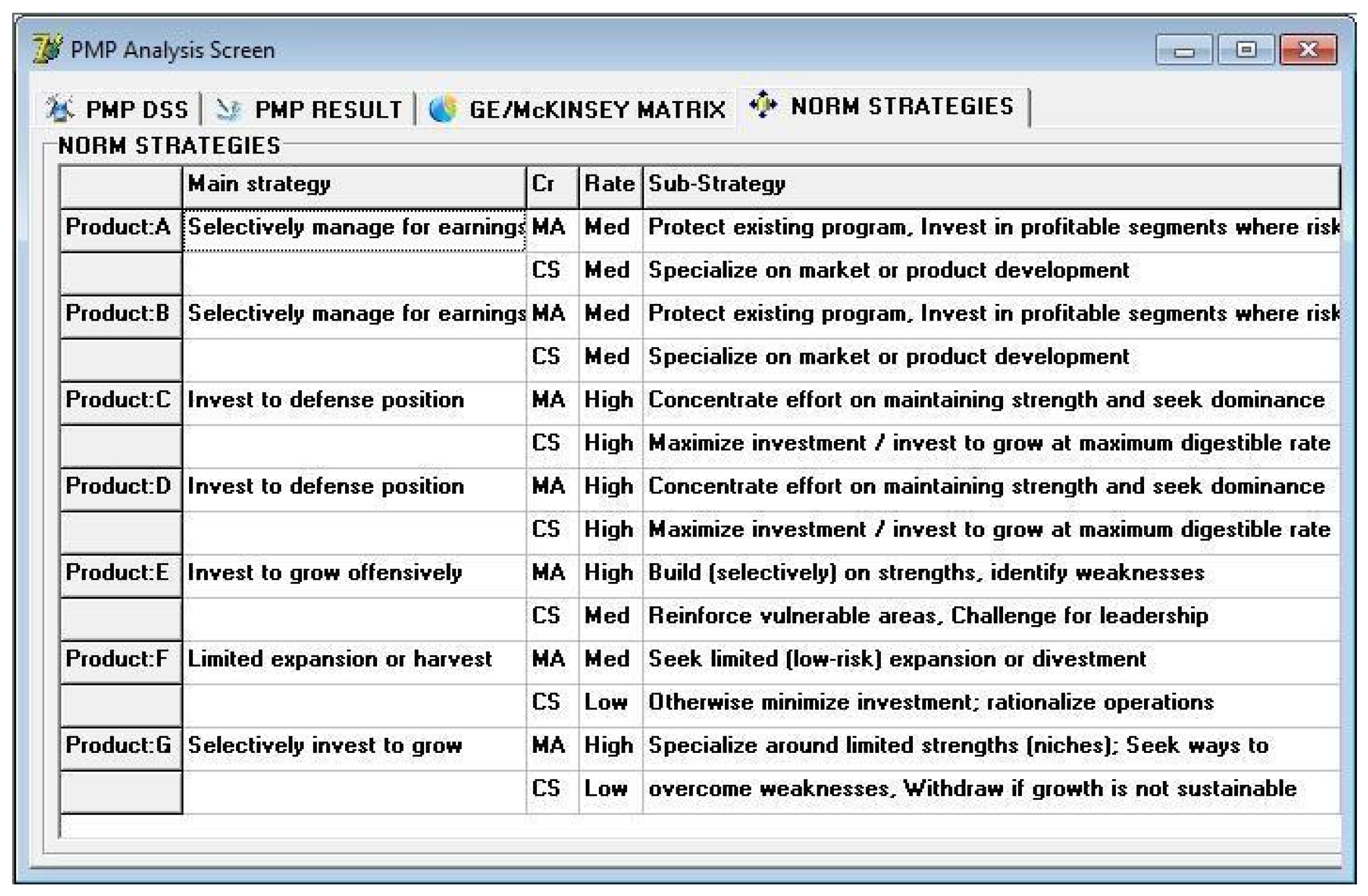
Appendix B. The Norm Strategies of the GE/McKinsey Screening Matrix

Invest to defend positionNorm Strategies
 Market Attractiveness
 Competitive Strength
High
High
Concentrate efforts on maintaining strength and seek dominance
Maximize investment/invest to grow at the maximum digestible rate
Invest to grow offensively
 Market Attractiveness
 Competitive Strength
High
Med
Build (selectively) on strengths, identify weaknesses
Reinforce vulnerable areas. Challenge for leadership
Invest to grow offensively
 Market Attractiveness
 Competitive Strength
Med
High
Identify attractive segments (growth areas) and invest in them
Build up the ability to counter competition
Focus on raising productivity for profitability
Selectively invest to grow
 Market Attractiveness
 Competitive Strength
High
Low
Specialize around limited strengths (niches)
Seek ways to overcome weaknesses
Withdraw if growth is not sustainable
Selectively manage earnings
 Market Attractiveness
 Competitive Strength
Med
Med
Protect the existing program
Invest in profitable segments where the risk is relatively low
Specialize in market or product development
Selectively protect and refocus
 Market Attractiveness
 Competitive Strength
Low
High
Defend strengths; manage for current earnings
Concentrate on attractive segments
Limited expansion or harvest
 Market Attractiveness
 Competitive Strength
Med
Low
Seek limited (low-risk) expansion or divestment
Otherwise, minimize investment; rationalize operations
Manage for earnings
 Market Attractiveness
 Competitive Strength
Low
Med
Prune unprofitable segments and upgrade the product line
Protect the company’s position in the most profitable segments
Minimize investment
Harvest or divest
 Market Attractiveness
 Competitive Strength
Low
Low
Cut fixed costs and avoid investment
Divest at a time that will maximize the cash value

References

  1. Komijan, A.R.; Aryanezhad, M.B.; Makui, A. A new heuristic approach to solve product mix problems in a multi-bottleneck system. J. Ind. Eng. Int. Islam. Azad Univ. 2009, 5, 46–57. [Google Scholar]
  2. Goldratt, E.M. What is This Thing Called Theory of Constraints and How Should It Be Implemented? North River Press: Croton-on-Hudson, NY, USA, 1990. [Google Scholar]
  3. Balakrishnan, J.; Cheng, C.H. Discussion: Theory of constraints and linear programming: A re-examination. Int. J. Prod. Res. 2000, 38, 1459–1463. [Google Scholar] [CrossRef]
  4. Fredendall, L.D.; Lea, B.R. Improving the product mix heuristic in the theory of constraints. Int. J. Prod. Res. 1997, 35, 1535–1544. [Google Scholar] [CrossRef]
  5. Lee, T.N.; Plenert, G. Optimizing theory of constraints when new product alternatives exist. Prod. Inventory Manag. J. 1993, 34, 51–57. [Google Scholar]
  6. Luebbe, R.L.; Finch, B.J. Theory of constraints and linear programming: A comparison. Int. J. Prod. Res. 1992, 30, 1471–1478. [Google Scholar] [CrossRef]
  7. Plenert, G. Optimizing theory of constraints when multiple constrained resources exist. Eur. J. Oper. Res. 1993, 70, 126–133. [Google Scholar] [CrossRef]
  8. Wu, K.; Zheng, M.; Shen, Y. A generalization of the Theory of Constraints: Choosing the optimal improvement option with consideration of variability and costs. IISE Trans. 2020, 52, 276–287. [Google Scholar] [CrossRef]
  9. Blackstone, J.H. Theory of constraints—A status report. Int. J. Prod. Res. 2001, 39, 1053–1080. [Google Scholar] [CrossRef]
  10. Goldratt, E.M. The Haystack Syndrome: Sifting Information out of the Data Ocean; North River Press: Croton-on-Hudson, NY, USA, 1990. [Google Scholar]
  11. Goldratt, E.M.; Cox, J. The Goal: A Process of Ongoing Improvement; 25th anniversary ed.; North River Press: Great Barrington, MA, USA, 2008. [Google Scholar]
  12. Lea, B.R.; Fredendall, L.D. The impact of management accounting, product structure, product mix algorithm, and planning horizon on manufacturing performance. Int. J. Prod. Econ. 2002, 79, 279–299. [Google Scholar] [CrossRef]
  13. Patterson, M.C. The product mix decision: A comparison of theory of constraints and labor-based management accounting. Prod. Inventory Manag. J. 1992, 33, 80–85. [Google Scholar]
  14. Finch, B.J.; Luebbe, R.L. Response to ‘theory of constraints and linear programming: A re-examination’. Int. J. Prod. Res. 2000, 38, 1465–1466. [Google Scholar] [CrossRef]
  15. Low, T.J. Do we really need product cost? The theory of constraints alternative. Corp. Controll. 1992, 5, 26–36. [Google Scholar]
  16. Mabin, V.J.; Davies, J. Framework for understanding the complementary nature of TOC frames: Insights from the product mix dilemma. Int. J. Prod. Res. 2003, 41, 661–680. [Google Scholar] [CrossRef]
  17. Linhares, A. Theory of constraints and the combinatorial complexity of the product-mix decision. Int. J. Prod. Econ. 2009, 121, 121–129. [Google Scholar] [CrossRef]
  18. Aryanezhad, M.B.; Komijan, A.R. An improved algorithm for optimizing product mix under the theory of constraints. Int. J. Prod. Res. 2004, 42, 4221–4233. [Google Scholar] [CrossRef]
  19. Maday, C.J. Proper use of constraint management. Prod. Inventory Manag. J. 1994, 35, 84. [Google Scholar]
  20. Posnack, A.J. Theory of constraints: Improper applications yield improper conclusions. Prod. Inventory Manag. J. 1994, 35, 85–86. [Google Scholar]
  21. Hsu, T.C.; Chung, S.H. The TOC-based algorithm for solving product mix problems. Prod. Plan. Control 1998, 9, 36–46. [Google Scholar] [CrossRef]
  22. Onwubolu, G.C.; Mutingi, M. A genetic algorithm approach to the theory of constraints product mix problems. Prod. Plan. Control 2001, 12, 21–27. [Google Scholar] [CrossRef]
  23. Onwubolu, G.C.; Mutingi, M. Optimizing the multiple constrained resources product mix problem using genetic algorithms. Int. J. Prod. Res. 2001, 39, 1897–1910. [Google Scholar] [CrossRef]
  24. Onwubolu, G.C. Tabu search-based algorithm for the TOC product mix decision. Int. J. Prod. Res. 2001, 39, 2065–2076. [Google Scholar] [CrossRef]
  25. Bhattacharya, A.; Vasant, P.; Sarkar, B.; Mukherjee, S.K. A fully fuzzified, intelligent theory of constraints product-mix decision. Int. J. Prod. Res. 2007, 46, 789–815. [Google Scholar] [CrossRef]
  26. Mishra, N.; Tiwari, M.; Shankar, R.; Chan, F. Hybrid tabu-simulated annealing based approach to solve multi-constraint product mix decision problem. Expert Syst. Appl. 2005, 29, 446–454. [Google Scholar] [CrossRef]
  27. Singh, R.K.; Prakash, K.S.; Tiwari, M.K. Psycho-clonal based approach to solve a TOC product mix decision problem. Int. J. Adv. Manuf. Technol. 2006, 29, 1194–1202. [Google Scholar] [CrossRef]
  28. Wang, J.Q.; Sun, S.D.; Si, S.B.; Yang, H.A. Theory of constraints product mix optimisation based on immune algorithm. Int. J. Prod. Res. 2009, 47, 4521–4543. [Google Scholar] [CrossRef]
  29. Ray, A.; Sarkar, B.; Sanyal, S. The TOC-based algorithm for solving multiple constraint resources. IEEE Trans. Eng. Manag. 2010, 57, 301–309. [Google Scholar] [CrossRef]
  30. Wang, J.Q.; Zhang, Z.T.; Chen, J.; Guo, Y.Z.; Wang, S.; Sun, S.D.; Qu, T.; Huang, G.Q. The TOC-based algorithm for solving multiple constraint resources: A re-examination. IEEE Trans. Eng. Manag. 2014, 61, 138–146. [Google Scholar] [CrossRef]
  31. Atli, Y.V. Determination of labour cost at cotton yarn manufacturing companies: A sampling [Turkish]. Tekst. Maraton 2004, 14, 66–67. [Google Scholar]
  32. Jiao, J.; Zhang, Y. Product portfolio planning with customer-engineering interaction. IIE Trans. 2005, 37, 801–814. [Google Scholar] [CrossRef]
  33. Kieltyka, L.; Hiep, P.M.; Dao MT, H.; Minh, D.T. Comparative analysis of business strategy of Hung Thinh and Novaland real estate developers using McKinsey matrix. Int. J. Multidiscip. Res. Growth Eval. 2022, 3, 175–180. [Google Scholar]
  34. Jang, H.S.; Choi, S.I.; Kim, W.Y.; Chang, C.K. Strategic selection of green construction products. KSCE J. Civ. Eng. 2012, 16, 1115–1122. [Google Scholar] [CrossRef]
  35. Zihare, L.; Blumberga, D. Market opportunities for cellulose products from combined renewable resources. Environ. Clim. Technol. 2017, 19, 33–38. [Google Scholar] [CrossRef]
  36. Al-Sharrah, G.K.; Hankinson, G.; Elkamel, A. Decision-making for petrochemical planning using multiobjective and strategic tools. Chem. Eng. Res. Des. 2006, 84, 1019–1030. [Google Scholar] [CrossRef]
  37. Olhager, J.; Wikner, J. Production planning and control tools. Prod. Plan. Control 2000, 11, 210–222. [Google Scholar] [CrossRef]
  38. Skinner, W. Manufacturing-Missing Link in Corporate Strategy. Harv. Bus. Rev. 1969, 47, 136–145. [Google Scholar]
  39. Moore, R. Making Common Sense Common Practice; Butterworth-Heinemann: Amsterdam, The Netherlands, 2004. [Google Scholar] [CrossRef]
  40. Baki, S.M.; Cheng, J.K. A linear programming model for product mix profit maximization in a small medium enterprise company. Int. J. Ind. Manag. (IJIM) 2021, 9, 64–73. [Google Scholar]
  41. Jaegler, Y.; Jaegler, A.; Mhada, F.Z.; Trentesaux, D.; Burlat, P. A new methodological support for control and optimization of manufacturing systems in the context of product customization. J. Ind. Prod. Eng. 2021, 38, 341–355. [Google Scholar] [CrossRef]
  42. Chanda, R.; Pabalkar, V.; Gupta, S. A study on application of linear programming on product mix for profit maximization and cost optimization. Indian J. Sci. Technol. 2022, 15, 1067–1074. [Google Scholar] [CrossRef]
  43. De Jesus Pacheco, D.A.; Junior, J.A.V.A.; de Matos, C.A. The constraints of theory: What is the impact of the Theory of Constraints on Operations Strategy? Int. J. Prod. Econ. 2021, 235, 107955. [Google Scholar] [CrossRef]
  44. Dombrowski, U.; Intra, C.; Zahn, T.; Krenkel, P. Manufacturing strategy–a neglected success factor for improving competitiveness. Procedia CIRP 2016, 41, 9–14. [Google Scholar] [CrossRef]
  45. Niski, A.; Krause, S.; Drusche, O. The sustainable corporate strategy in industrial goods markets. Okol. Wirtsch.-Fachz. 2020, 33, 30–37. [Google Scholar] [CrossRef]
  46. Patil, P.P.; Narkhede, B.E.; Akarte, M.M. Pattern of manufacturing strategy implementation and implications on manufacturing levers and manufacturing outputs and business performance. Int. J. Indian Cult. Bus. Manag. 2015, 10, 157–177. [Google Scholar] [CrossRef]
  47. Sarmiento, R.; Thurer, M.; Whelan, G. Rethinking Skinner’s model: Strategic trade-offs in products and services. Manag. Res. Rev. 2016, 39, 1199–1213. [Google Scholar] [CrossRef]
  48. Dangayach, G.S.; Deshmukh, S.G. Manufacturing strategy: Literature review and some issues. Int. J. Oper. Prod. Manag. 2001, 21, 884–932. [Google Scholar]
  49. Dohale, V.; Gunasekaran, A.; Akarte, M.M.; Verma, P. Twenty-five years’ contribution of “Benchmarking: An International Journal” to manufacturing strategy: A scientometric review. Benchmarking Int. J. 2020, 27, 2887–2908. [Google Scholar] [CrossRef]
  50. Dohale, V.; Gunasekaran, A.; Akarte, M.M.; Verma, P. 52 Years of manufacturing strategy: An evolutionary review of literature (1969–2021). Int. J. Prod. Res. 2022, 60, 569–594. [Google Scholar] [CrossRef]
  51. Dohale, V.; Akarte, M.M.; Verma, P. Systematic review of manufacturing strategy studies focusing on congruence aspect. Benchmarking Int. J. 2022, 29, 2665–2690. [Google Scholar]
  52. Das, S.; Canel, C. Linking manufacturing and competitive strategies for successful firm performance: A review and reconceptualization. J. Strategy Manag. 2022, 16, 148–172. [Google Scholar] [CrossRef]
  53. Čižman, A.; Černetič, J. Improving competitiveness in veneers production by a simple-to-use DSS. Eur. J. Oper. Res. 2004, 156, 241–260. [Google Scholar] [CrossRef]
  54. Kotler, P.; Armstrong, G. Principles of Marketing; Pearson Education: Harlow, UK, 2010. [Google Scholar]
  55. Saaty, T.L. The Analytic Hierarchy Process: Planning, Priority Setting, Resource Allocation; McGraw-Hill International Book Co.: New York, NY, USA; London, UK, 1980. [Google Scholar]
  56. Vargas, L.G. An Overview of the Analytic Hierarchy Process and its Applications. Eur. J. Oper. Res. 1990, 48, 2–8. [Google Scholar] [CrossRef]
  57. Saaty, T.L. Decision Making with the Analytic Hierarchy Process. Int. J. Serv. Sci. 2008, 1, 83–98. [Google Scholar] [CrossRef]
  58. Ishizaka, A.; Labib, A. Review of the Main Developments in the Analytic Hierarchy Process. Expert Syst. Appl. 2011, 38, 14336–14345. [Google Scholar] [CrossRef]
  59. Glover, F. Tabu search—Part I. ORSA J. Comput. 1989, 1, 190–206. [Google Scholar] [CrossRef]
Figure 1. Data flow diagram of the proposed methodology.
Applsci 13 12191 g001
Figure 2. Main criteria and sub-criteria of AHP for PMP [29]. © 2010 IEEE. Reprinted, with permission, from Ray, A.; Sarkar, B.; Sanyal, S. The TOC-based algorithm for solving multiple constraint resources. IEEE Trans. Eng. Manag. 2010, 57.
Applsci 13 12191 g002
Figure 3. AHP-TOC heuristic execution procedure.
Applsci 13 12191 g003
Figure 4. The GE/McKinsey screen matrix.
Applsci 13 12191 g004
Figure 5. The derived norm strategies for a product portfolio.
Applsci 13 12191 g005
Table 1. Saaty’s nine-point scale for pairwise comparison.
Extreme ImportanceVery Strong ImportanceStrong ImportanceModerate ImportanceEqual ImportanceModerate ImportanceStrong ImportanceVery Strong ImportanceExtreme Importance
9:18:17:16:15:14:13:12:11:11:21:31:41:51:61:71:81:9
ResourcesApplsci 13 12191 i001Applsci 13 12191 i001Applsci 13 12191 i001Applsci 13 12191 i001Applsci 13 12191 i001Applsci 13 12191 i001Applsci 13 12191 i001Applsci 13 12191 i001Applsci 13 12191 i001Applsci 13 12191 i001Applsci 13 12191 i001Applsci 13 12191 i001Applsci 13 12191 i001Applsci 13 12191 i001Applsci 13 12191 i001Applsci 13 12191 i001Applsci 13 12191 i001Profit
Table 2. PMP dataset.
SBUDi
(ton)
CMi ($/ton)CMi/ti8 (seq1)Processing Times on Resources (min)
S1S2S3S4S5S6S7S8S9
A81280063.64343331243237354436
B52285055.88403836273643405142
C57290047.54474443324350476149
D290290043.28524947354755526754
E69370044.58646159445969658367
F84400038.837975725473858010383
G63550041.3510398947195111104133108
Required capacity TRCj40,13438,05036,50527,36736,73342,92740,43151,88141,952
Available capacity βj41,76041,76041,76041,76041,76041,76041,76041,76041,760
Difference dj16263710525514,3935027−11671329−10,121−192
Constraint resources CR BN2 BN1BN3
Actual or max. available capacity bj40,13438,05036,50527,36736,73341,76040,43141,76041,760
Table 3. Decision matrix for the PMP.
ResourceProfitPriority Vector
Resource11/20.333
Profit210.667
Table 4. Normalized processing time (pij).
SBUB04
(ri)
B05—Normalized Processing Times (pij)B08
(hi)
B09 (Wi)seq2
S1S2S3S4S5S6S7S8S9
A0.1140.0810.0830.0810.0840.0830.0820.0830.0810.0820.2190.1492
B0.1160.0950.0950.0940.0940.0940.0960.0950.0940.0960.1890.1403
C0.1180.1120.1110.1130.1110.1120.1110.1110.1130.1120.1610.1326
D0.1180.1240.1230.1230.1220.1220.1220.1230.1240.1230.1460.1277
E0.1500.1530.1530.1540.1530.1530.1530.1540.1530.1530.1170.1395
F0.1620.1890.1880.1880.1880.1900.1890.1890.1900.1890.0950.1404
G0.2230.2460.2460.2460.2470.2470.2470.2460.2450.2460.0720.1731
B07 (qj):0.1160.1100.1060.0790.1060.1210.1170.1210.121
Table 5. Overview of Step B10-b’s initial MPS and bottleneck capacity.
S6S8S9
SBUDixiBusyIdleBusyIdleBusyIdle
A8181299738,763356438,196291638,844
B5252223636,527265235,544218436,660
C5757285033,677347732,067279333,867
E6969476128,916572726,340462329,244
D29029015,95012,96619,430691015,66013,584
G635156617305678312755088076
F84185722010324837993
Total Profit: 1921,100
Table 6. Identification of the Q candidates.
SequenceStepPriority Sequence
seq1A03A> B> C> E> D> G> F
seq2B09G> A> B> F> E> C> D
Q Candidates →Q1 Q2
P Candidates P5 P4 P3 P2 P1
Table 7. Neighboring moves of one-way TS and change in profit.
P CandidatesQ Candidates
IterationDCEBAGFS8ProfitTabu
0290576952815101271,917,100
128957695281520611,919,700
229056695281520551,919,700
329057685281520771,918,900X
429057695181520451,919,750
529057695280520381,919,800
628956695281521191,920,800
72905668528153051,921,500
829057685181521251,920,050X
929057695180520891,916,950X
102895769528052121,920,900X
1128957685281530111,921,500
122905669518152131,920,850X
3128956685180540341,918,450X
Table 8. The pairs of average market attractiveness and competitive strength values.
SBUMarket
Attractiveness
Competitive
Strength
DiImportance
Value
Importance Order
A4.53813.755
B4.43.5523.954
C5.95575.452
D6.262906.101
E5.34.6694.953
F4.552.2843.377
G5.51.5633.506
Importance order: D > C > E > B > A > G > F
Table 9. Step B12—the identification of P and Q candidates.
SequenceStepPriority Sequence
seq2B09G> A> F> B> E> C> D
seq3B11A> B> C> E> D> G> F
Q Candidates → Q1
P Candidates P3 P1 P2
Disclaimer/Publisher’s Note: The statements, opinions and data contained in all publications are solely those of the individual author(s) and contributor(s) and not of MDPI and/or the editor(s). MDPI and/or the editor(s) disclaim responsibility for any injury to people or property resulting from any ideas, methods, instructions or products referred to in the content.

